A Numerical Study of the Non-Ideal Behavior, Parameters, and Novel Applications of an Electrothermal Plasma Source.

(1)

Abstract

WINFREY, A. LEIGH. A Numerical Study of the Non-Ideal Behavior, Parameters, and Novel Applications of an Electrothermal Plasma Source. (Under the direction of Dr. A.V. Saveliev and Dr. J.G. Gilligan.)

Electrothermal plasma sources have numerous applications including hypervelocity launchers, fusion reactor pellet injection, and space propulsion systems. The time evolu-tion of important plasma parameters at the source exit is important in determining the suitability of the source for different applications.

In this study a capillary discharge code has been modified to incorporate non-ideal behavior by using an exact analytical model for the Coulomb logarithm in the plasma electrical conductivity formula. Actual discharge currents from electrothermal plasma experiments were used and code results for both ideal and non-ideal plasma models were compared to experimental data, specifically the ablated mass from the capillary and the electrical conductivity as measured by the discharge current and the voltage.

Electrothermal plasma sources operating in the ablation-controlled arc regime use discharge currents with pulse lengths between 100 µs to 1 ms. Faster or longer or ex-tended flat-top pulses can also be generated to satisfy various applications of ET sources. Extension of the peak current for up to an additional 1000 µs was tested. Calculations for non-ideal and ideal plasma models show that extended flattop pulses produce more ablated mass, which scales linearly with increased pulse length while other parameters remain almost constant

(2)

materials synthesis, and the physics of complex mixed plasmas. This source is a capillary discharge where the ablation liner is made from segments of different materials instead of a single sleeve. This system should allow for the modeling and characterization of the growth plasma as it provides all materials needed for fabrication through the same method.

An ablation-free capillary discharge computer code has been developed to model plasma flow and acceleration of pellets for fusion fueling in magnetic fusion reactors. Two case studies with and without ablation, including different source configurations have been studied here. Velocities necessary for fusion fueling have been achieved.

(3)

c

(4)

A Numerical Study of the Non-Ideal Behavior, Parameters, and Novel Applications of an Electrothermal Plasma Source

by

A. Leigh Winfrey

A dissertation submitted to the Graduate Faculty of North Carolina State University

in partial fulfillment of the requirements for the Degree of

Doctor of Philosophy

Mechanical Engineering

Raleigh, North Carolina 2010

APPROVED BY:

Dr. A.V. Saveliev

Co-Chair, Advisory Committee

Dr. J.G. Gilligan

Co-Chair, Advisory Committee

Dr. T. Echekki Dr. A.V. Kuznetsov

(5)

Dedication

(6)

Biography

(7)

Acknowledgements

I would like to begin by acknowledging and thanking my committee. First I would like to thank my Co-Chairs Dr. Gilligan and Dr. Saveliev for their expertise, direction, support, and generosity with their time during this research. My thanks to Dr. Kuznetsov for his enthusiasm in teaching and insights into heat transfer and flow behavior. Also, my thanks to Dr. Echekki for giving me a deeper understanding of chemical processes and his creative suggestions for my research. Lastly, I would like to thank Dr. Bourham for sharing his passion for plasma physics and his mentorship through out my graduate studies.

(8)

List of Tables

Table 3.1 Summary of predicted plasma parameters using the ideal and non-ideal models as well as the measured ablated mass . . . 32 Table 4.1 Code run time for ideal plasma model for 11, 25, and 48 nodes cases 42 Table 6.1 ETFLOW results for silicon carbide formation using an eleven

ment source composed of ten carbon segments and one silicon seg-ment, where the location of the silicon segment was varied for each experiment. Results are listed by silicon segment location; Si#11 is the segment at the source exit. . . 91 Table 6.2 ETFLOW results for silicon carbide formation using a twenty five

segment source composed of twenty four carbon segments and one silicon segment, where the location of the silicon segment was varied for each experiment. Results are listed by silicon segment location; Si#25 is the segment at the source exit. . . 92 Table 6.3 ETFLOW results for silicon carbide formation using an eleven

seg-ment source, where the location and number of the silicon segseg-ments was varied for each experiment. Results are listed by silicon segment quantity and location. . . 94 Table 6.4 ETFLOW results for silicon carbide formation using an eleven

seg-ment source, where the location and number of the carbon segseg-ments was varied for each experiment. Results are listed by carbon seg-ment quantity and location. . . 101 Table 6.5 ETFLOW results for silicon carbide formation using a twenty five

segment source, where the location and number of the carbon seg-ments was varied for each experiment. Results are listed by silicon segment quantity and location. . . 103 Table 6.6 Case 1: Configuration of the source segments for MoS2Ti fabrication.115

Table 6.7 Case 1: Ablated mass of each element and plasma composition. . 115 Table 6.8 Case 2: Configuration of the source segments for MoS2Ti fabrication.116

Table 6.9 Case 2: Ablated mass of each element and plasma composition. . 116 Table 6.10 Case 3: Configuration of the source segments for MoS2Ti fabrication.117

(12)

Table 6.17 Case 6: Ablated mass of each element and plasma composition. . 120 Table 7.1 Pellet exit velocity for different barrel lengths for 2 cm and 18 cm

sources. . . 145 Table 7.2 Pellet exit velocity for different barrel lengths for 18cm sources

using a 285µs current pulse peaking to 40 kA at 85 µs . . . 148 Table 7.3 Pellet exit velocity for different barrel lengths for 9 and 18 cm

(13)

List of Figures

Figure 1.1 A schematic of an electrothermal capillary discharge showing the cathode, anode, source material, and plasma jet. . . 4 Figure 1.2 A schematic of the electrothermal plasma facility PIPE showing

the source and pulse forming network. . . 6 Figure 1.3 Sample current traces of twelve PIPE shots . . . 7 Figure 2.1 Change in k versus n for the Reynolds number for friction factor

calculation . . . 18 Figure 3.1 Code predictions of the total ablated mass for both the ideal and

non-ideal models and the experimentally measured values as a func-tion of the peak discharge current . . . 24 Figure 3.2 Peak plasma temperature at the capillary exit for both the ideal

and non-ideal models as a function of the peak discharge current . 26 Figure 3.3 Peak electron number density at the capillary exit for both the

ideal and non-ideal models as a function of the peak discharge current. 28 Figure 3.4 Peak total number density at the capillary exit for both the ideal

and non-ideal models as a function of the peak discharge current. 29 Figure 3.5 Peak plasma pressure at the capillary exit for both the ideal and

non-ideal models as a function of the peak discharge current . . . 31 Figure 3.6 Plasma bulk velocity at the capillary exit for both the ideal and

non-ideal models as a function of the peak discharge current . . . 33 Figure 3.7 Plasma electrical conductivity as a function of discharge time for

both the ideal and non-ideal models as compared to the measured value for shot P215 (I=18.04kA, E=2.42kJ) . . . 35 Figure 3.8 Plasma electrical conductivity as a function of discharge time for

both the ideal and non-ideal models as compared to the measured value for shot P204 (I=38.98kA, E=5.91kJ) . . . 36 Figure 3.9 Comparison between code predictions of the plasma electrical

con-ductivity for the ideal and non-ideal models and the measured . . 38 Figure 4.1 Discharge current of Shot P228, peaking 28.93kA at 30 µs of the

discharge time. . . 41 Figure 4.2 Plasma temperature in time at the source exit, 11 nodes (length=8.18

(14)

Figure 4.4 Plasma temperature in time at the source exit, 48 nodes (length=1.83 mm). . . 44 Figure 4.5 Pressure axial distribution at various times during the discharge,

11 nodes. . . 44 Figure 4.6 Pressure axial distribution at various times during the discharge,

25 nodes. . . 45 Figure 4.7 Pressure axial distribution at various times during the discharge,

48 nodes. . . 45 Figure 4.8 Pressure drop along the capillary axis as a function of the discharge

current. . . 46 Figure 4.9 Axial distribution of plasma temperature inside the capillary at

various times during the discharge . . . 47 Figure 4.10 Axial distribution of plasma electrical conductivity inside the

cap-illary at various times during the discharge. . . 48 Figure 4.11 Axial distribution of plasma electron number density, Ne, inside

the capillary at various times during the discharge. . . 49 Figure 4.12 Axial distribution of the second ionization state number density,

N1, inside the capillary at various times during the discharge. . . . 50

Figure 4.13 Axial distribution of the second ionization state number density,

N2, inside the capillary at various times during the discharge. . . . 51

Figure 4.14 Axial distribution of plasma neutral number density, N0, inside

the capillary at various times during the discharge. . . 52 Figure 4.15 Axial distribution of the total plasma number density, Np, inside

the capillary at various times during the discharge. . . 52 Figure 4.16 Time-dependent variation of the number densities at the capillary

exit. . . 53 Figure 4.17 Axial distribution of the bulk velocity at various times during the

discharge. . . 54 Figure 4.18 Time dependent variation of the plasma bulk velocity at the

cap-illary exit. . . 54 Figure 5.1 Illustration of ideal interior ballistics profiles for electrothermal

launchers. . . 58 Figure 5.2 Schematic of the equivalent circuit elements for pulse generation. 60 Figure 5.3 Discharge current without flattop extension (zero extension) and

with 100 µs extension. . . 62 Figure 5.4 Total ablated mass as a function of time for zero and 100µs peak

(15)

Figure 5.6 Plasma kinetic temperatures at the source exit as a function of time for zero and 100µs peak current extension for both ideal and nonideal model code results. . . 65 Figure 5.7 Peak plasma kinetic temperatures at the source exit as a function

of the time extension of the peak discharge current for both the ideal and nonideal models. . . 66 Figure 5.8 Plasma pressure at the source exit as a function of time for zero and

100 µs peak current extension for both ideal and nonideal model code results. . . 67 Figure 5.9 Peak plasma kinetic temperatures at the source exit as a function

of the time extension of the peak discharge current for both the ideal and nonideal models. . . 68 Figure 5.10 Peak electron and total number densities at the source exit as a

function of the time extension of the peak discharge current for both the ideal and nonideal models. . . 69 Figure 5.11 Plasma bulk velocities at the source exit as a function of time for

zero and 100µs peak current extension for both ideal and nonideal model code results. . . 70 Figure 5.12 Peak plasma bulk velocities at the source exit as a function of the

time extension of the peak discharge current for both the ideal and nonideal models. . . 71 Figure 5.13 Predicted ballisitics for flattop pulse length extension. . . 72 Figure 6.1 Schematic of the electrothermal segmented plasma source (ETSPS). 76 Figure 6.2 Time history of the plasma temperature at the source exit for

tested metals. . . 79 Figure 6.3 Time history of the plasma pressure at the source exit for tested

metals. . . 80 Figure 6.4 Time history of the plasma total number density at the source exit

for tested metals. . . 81 Figure 6.5 Time history of the plasma electron number density at the source

exit for tested metals. . . 82 Figure 6.6 Picture of the experimental ET source showing the main chamber,

the ET source and the substrate stand. . . 83 Figure 6.7 Optical emission spectra of the Mo plasma jet with elemental lines

(16)

Figure 6.11 Scanning electron microscopy and EDXA of the sample surface showing 95.87%wt for deposited molybdenum particulates. . . 88 Figure 6.12 ETFLOW results for silicon carbide formation using an eleven

segment source composed of ten carbon segments and one silicon segment, where the location of the silicon segment was varied for each experiment. . . 90 Figure 6.13 ETFLOW results for silicon carbide formation using a twenty five

segment source composed of twenty four carbon segments and one silicon segment, where the location of the silicon segment was varied for each experiment. . . 93 Figure 6.14 ETFLOW results for silicon carbide formation using an eleven

node source with variation in the placement and composition of silicon segments. . . 95 Figure 6.15 Time history of plasma temperature at the source exit for increased

number of silicon segments. . . 97 Figure 6.16 Total number density over time at the source exit for increasing

Si content. . . 98 Figure 6.17 Time history of kinetic pressure at the source exit for increased

number of silicon segments. . . 99 Figure 6.18 Effect of increased silicon segments on the mixing with carbon in

a 4mm bore, 90-mm long, 11 segments ET source. . . 100 Figure 6.19 Plasma composition of a twenty five node electrothermal source as

a function of the number of silicon segments in the source. . . 102 Figure 6.20 Axial distribution of the plasma kinetic temperature for a

seg-mented source with one silicon segment in the middle and all others are carbon. . . 104 Figure 6.21 Axial distribution of the plasma pressure for a segmented source

with one silicon segment in the middle and all others are carbon. . 106 Figure 6.22 Axial distribution of the plasma pressure for a segmented source

with 4 silicon segments at the source entry followed by 7 carbon segments. . . 107 Figure 6.23 Axial distribution of the plasma pressure for a 4mm bore, 90-mm

long segmented source with 4 silicon segments at the source entry followed by 7 carbon segments. . . 108 Figure 6.24 Axial distribution of the plasma kinetic temperature for a

seg-mented copper capillary source with one Al2O3 as the 2nd segment

at the source entry. . . 110 Figure 6.25 Axial distribution of the plasma kinetic pressure for a segmented

(17)

Figure 6.26 Axial distribution of the plasma kinetic temperature of MoSTi Case 5. . . 121 Figure 6.27 Axial distribution of the total number density of the MoSTi Case 5.122 Figure 7.1 A cross section of the International Thermonuclear Test Reactor

ITER [86]. . . 126 Figure 7.2 ITER vacuum vessel (top) and ITER diagnostics duct assembly

(bottom) showing several ducts and ports for various instrumenta-tion[87]. . . 128 Figure 7.3 Schematic of an ablation-dominated electrothermal mass accelerator.130 Figure 7.4 Schematic of an ablation-free electrothermal fusion pellet

acceler-ator with gas injection and a pellet formation station. . . 134 Figure 7.5 Illustration of installing an electrothermal pellet accelerator on a

large fusion reactor like ITER. . . 135 Figure 7.6 Schematic showing the differences in nucleation and growth of (a)

microcrystalline diamond with large growth domains, (b) nanocrys-talline diamond with smaller domains and relatively thick grain boundaries, and (c) ultra-nanocrystalline diamond films with min-imum achievable grain size and grain boundary thickness [77,78]. . 137 Figure 7.7 SEM (left) and AFM (right) images of a NCD grown in Ar-H-CH4

microwave plasma by plasma enhanced chemical vapor deposition (PECVD) technique [77]. . . 139 Figure 7.8 Axial distribution of the plasma kinetic temperature inside the

source and barrel. . . 141 Figure 7.9 Axial distribution of the plasma total number density inside the

source and barrel. . . 142 Figure 7.10 Axial distribution of the plasma kinetic pressure inside the source

and barrel. . . 143 Figure 7.11 Discharge current for pellet acceleration tests, peaking 20 kA at

85µs of the discharge time with full active pulse length of 285 µs. 144 Figure 7.12 Pellet exit velocity as a function of the barrel length for 9 cm and

18 cm sources using a 285µs current pulse peaking to 20 kA at 85

µs. . . 146 Figure 7.13 Axial distribution of the pressure in the source and barrel, at

(18)

Figure 7.16 Time history of the pellet displacement for the 9, 18 and 72 cm barrels. . . 151 Figure 7.17 Schematic of the electrothermal source concept with LiH capsules

in a sealed carousel. . . 156 Figure 7.18 Comparison of the pellet exit velocity as a function of the barrel

length for 9 and 18cm source using a 285µs current pulses peaking to 20 and 40 kA at 85µs. . . 158 Figure 8.1 Electron number density of a copper plasma at 20, 40, 60, and 80

µs. . . 172 Figure 8.2 Total number density of a copper plasma at 20, 40, 60, and 80 µs. 173 Figure 8.3 1st _{ionization number density of a copper plasma at 20, 40, 60,}

and 80µs. . . 174 Figure 8.4 2nd _{ionization number density of a copper plasma at 20, 40, 60,}

and 80µs. . . 174 Figure 8.5 Kinetic temperature of a copper plasma at 20, 40, 60, and 80µs. 175 Figure 8.6 Electrical conductivity of a copper plasma at 20, 40, 60, and 80µs. 176 Figure 8.7 Electron number density of a Lexan plasma at 20, 40, 60, and 80µs.178 Figure 8.8 1st ionization number density of a Lexan plasma at 20, 40, 60, and

80µs. . . 179 Figure 8.9 2nd _{ionization number density of a Lexan plasma at 20, 40, 60,}

and 80µs. . . 179 Figure 8.10 Total number density of a Lexan plasma at 20, 40, 60, and 80 µs. 180 Figure 8.11 Kinetic temperature of a Lexan plasma at 20, 40, 60, and 80 µs. . 181 Figure 8.12 Electrical conductivity of a Lexan plasma at 20, 40, 60, and 80 µs. 182 Figure 8.13 Electron number density of a SiC plasma at 20, 40, 60, and 80 µs. 183 Figure 8.14 1st _{ionization number density of a SiC plasma at 20, 40, 60, and}

80µs. . . 184 Figure 8.15 2nd _{ionization number density of a SiC plasma at 20, 40, 60, and}

(19)

Chapter 1 Introduction

1.1 Electrothermal Plasma Background

Electrothermal plasmas produced in capillary discharges have been investigated for var-ious applications that require the generation of high energy density electrothermal plas-mas. Capillary discharges produce high-density (1023_-1027_/m3_{) electrothermal plasmas}

with temperatures in the range of 1-5e V and are of interest in a variety of applications such as hypervelocity launch devices [1-3], fusion reactor pellet injectors [4,5], space propulsion systems [6], high heat flux sources [7,8], plasma plugs for combustion control [9], and pulsed thrusters for small satellites [10].

(20)

rail-used in contoured gap, coaxial plasma guns to accelerate 100-200 µg of a plasma with density above to 1023_/m3 _{to speeds greater than 200 km/s, which correlates to a Mach}

number greater than 10 [13]. Extensive research has been done on electrothermal chem-ical (ETC) launchers at the US Army Research Laboratory and other institutions. This work explores the interaction of electrothermal plasmas with solid and liquid propellants and the enhancement of burn rates for ETC launch devices [3,14-18].

The investigation of electrothermal plasma sources as pellet accelerators for fueling magnetic fusion tokamak reactors was explored experimentally and theoretically by Kin-cad et al [4, 19, 20] where they were able to launch 1.0 gm pellets to velocities in excess of 2 km/s; similarly Shcolnikov et. al. reported achieving 2 km/s for a 2.2 g pellets in their experiment [5]. Electrothermal plasma sources for space applications, thrusters, and arc heaters have also been studied by several groups. The early work of Wang et. al. on using electrothermal plasma sources for propulsion provided a study on the applicability of electrothermal systems for space-based orbit transfer [6]. Recent work by Edamitsu and Tahara provided experimental and numerical studies on the use of electrothermal pulsed plasma thrusters for small satellites [10].

(21)

In all applications of electrothermal plasmas generated by capillary discharges the behavior and parameters of the generated electrothermal plasma must be well charac-terized, predictable, and reproducible. In a capillary discharge the plasma is generated from the ablation of a liner material inside the capillary. Ablation results from driv-ing an arc through the confined channel, which radiates energy to the wall via thermal near-blackbody radiation.

The early study of Ibrahim on the ablation dominated polymethylmethacrylate arc, in which the author developed an analytical model for the ablation in confined capillary discharge, concluded that the temperature distribution in the high current arc is almost flat radially, therefore a 1-D model is sufficient to describe the physical processes in such discharges [21]. Time dependent, 1-D models were developed by others to investigate electrothermal plasmas; they differ from each other in the formulation of the set of governing equations and model assumptions [22-28]. Some 0-D models [29-30] and other scaling laws derived from 0-D models were also developed [31]. Plasma resistivity, in most models, is based on the sum of two collisional mechanisms, neutral and electron-ion colliselectron-ions with the later mostly taken from the Spitzer model with the correctelectron-ion factor that accounts for electron-electron interactions [32]. Electrothermal plasmas tend to be weakly non-ideal and some models provided corrections for the Coulomb logarithm with limited range of applicability, such as the model by Zollweg and Liebermann in which a numerically computed and fitted modified Coulomb logarithm was derived to account for non-ideal plasma behavior [33,34].

(22)

1.2 The Electrothermal Plasma Source

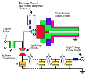
A schematic of an electrothermal plasma source is shown in Figure 1.1. The source is composed of an outer cylindrical grounded electrode, an insulator that houses the ab-lating, capillary sleeve, and an inner electrode. The source is powered by a pulse power system composed of high energy density capacitors that are discharged via an ignitron or a spark-gap switch. The energy radiated to the walls of the capillary is absorbed on the interior surface and causes ablation of the liner material which then forms a dense vapor of excited atoms and molecules dissociated from the wall. The ablated material is then ionized to form a plasma.

(23)

The energy radiated to the walls of the capillary is absorbed on the surface and causes ablation without a phase change from solid to liquid to vapor, therefore a dense vapor of excited atoms and molecules dissociated from the wall is formed. Further input of energy into the vapor will cause some of the atoms to become ionized, which gener-ates a low-temperature, high-density plasma. As the plasma temperature increases the plasma resistance drops, which in turn allows more current to pass through the confined channel. As the current increases more material is ablated and the plasma number den-sity increases, which results in increased kinetic pressure inside the source. This cycle continues until no more joule heating occurs.

The electrothermal plasma facility PIPE is used for this study to compare code results to experimentally measured parameters. Electrothermal plasmas are low-temperature (1-5 eV), high-density (1023_-1027_/m3_{) plasmas in near local thermodynamic equilibrium that}

radiate energy as blackbodies, or near blackbodies. These plasmas may depart from ideal behavior and fall in the non-ideal regime [33-37]. The PIPE facility has been used to assess the behavior of the plasma in comparison to the ideal and non-ideal models.

(24)

Figure 1.2: A schematic of the electrothermal plasma facility PIPE showing the source and pulse forming network.

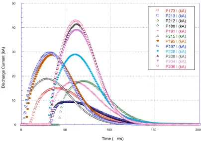
discharge current are important to precise predictions of any electrothermal plasma code [22-26]. Samples of the discharge current traces of the experimental shots are shown in Figure 1.3; the data acquisition system may be triggered at a point several microseconds prior to the discharge of the capacitor to ensure full acquisition of the discharge current and voltage traces.

(25)

(26)

1.3 Motivation and Goals of the Study

While electrothermal plasmas are useful in many applications, they have not been ex-tensively modeled for applications outside of ignitors for ETC guns. It is essential to understand the behavior, parameters, and characteristics in order to expand their range of applicability. This work expands the range of modeling capabilities for electrothermal plasmas in several new and important ways. A model for non-ideal plasma behavior has been incorporated, which allows for more realistic modeling of ET plasmas. Extensive studies on novel applications for electrothermal plasma use have been conducted compu-tationally using a new code. This program ETFLOW is based off of previous 0-D and 1-D ideal plasma codes. It is a 1-D and semi 2-D code that has improved usability and functionality over all previous codes. ETFLOW has been used here to study applications for which electrothermal plasmas are not currently in use, but which could benefit from the technology.

Specifically, the goals of this study are:

1. Develop a modified 1-D, time dependent electrothermal plasma computer code which incorporates a non-ideal plasma model in the resistivity equation for accurate calculation of the joule heating provided to the plasma. Compare the Spitzer ideal model and the Zaghloul non-ideal model to results from the PIPE device.

(27)

3. Study the effect of plasma non-ideality on the electrothermal plasma parameters and compare both the ideal and non-ideal model results to the experimental values in order assess if the plasma is idea, weakly non-ideal, or fully non-ideal.

4. Study the axial behavior of the plasma flow in the electrothermal discharge. 5. Study the effect of extended flat-top pulse length on the plasma parameters for

launch technology applications and mini-thrusters space applications.

6. Study the electrothermal plasma source with mixed materials in an Electrothermal Segmented Plasma Source, ETSPS, to evaluate synthesis of materials for possible electrothermal plasma deposition application.

7. Develop additional code to model and study the acceleration of small payloads. 8. Study the requirements for a 2-D, time dependent version of the code, ETFLOW

(28)

Chapter 2 Governing Equations of the Model

and the ETFLOW Code

(29)

2.1 Basic Assumptions of the Plasma Model

When developing a model for an electrothermal plasma source, one can make several simplifying assumptions. In a 1-D axial model, the radius of the capillary R is taken to be small with respect to its length L, so that the source has a very small aspect ratio

R/L. Here the dimensions are R=0.2 cm andL=9 cm so the aspect ratio is 0.022. The plasma parameters can be taken as constant, on average, over the cross section.

The ablated wall material in the source is assumed to be completely dissociated and the heat loss due to conduction is negligible, however, thermal conduction is included in the model and the code. Also, radiation transport is assumed only in the radial direction and is neglected in the axial direction. This can be safely ignored in this configuration because the radiation transport is responsible for the wall ablation in the radial direction but no radiation transport occurs during the plasma axial flow, and the plasma is relatively isothermal [21-28].

(30)

2.2 Conservation of Mass

By taking a slice of the source inner bore the behavior of the plasma can be examined analytically or computationally. The rate of change in the particle density is the difference between the rate at which particles are introduced into the cell from ablation of the wall and the rate at which particles enter or leave the cell, therefore the continuity equation must include the time rate of change of the number density of the ablated material from the cell wall and is given by [22]:

∂n

∂t = ˙na−

∂(vn)

∂z (2.1)

where n (atoms/m3_{) is the number density of the plasma particles, ˙}_n

a (atoms/m3) is

the time rate of change of the number density of ablated material from the cell wall, and v (m/s) is the plasma velocity. The ablation results from the surface radiation heat flux 2q00_rad (W/m2_{) reaching the inner surface of the capillary; the thermal radiation}

responsible for ablation must be transferred from surface to volumetric heat flux q000_rad

(W/m3) by multiplying the surface heat flux by 2πRl/πR2l to get q000_rad=2q00_rad/R. The time rate of change of the number density of ablated material from the wall is given by an equation that accounts for the ablation due to radiation heat flux from the plasma on the wall [29,40]:

˙

na=

2q00_rad HsubApR

(2.2)

whereq00_rad (W/m2_{) is the radiation heat flux from the plasma to the wall,}_A

p (kg/atom)

(31)

total energy required to dissociate the molecules into the plasma.

Since the arc is formed between the cathode inside the channel and the grounded anode, the arc will radiate its energy in the form of blackbody radiation to the wall of the inner sleeve inside the source, so the radiation heat flux is described by the Stefan-Boltzmann law [23,24,41]:

q_rad00 =σb Tplasma4 −T

4

vapor

(2.3)

where σb is the Stefan-Boltzmann constant, Tplasma is the skin temperature (K) of the

arc radiating to the wall, and Tvapor is the temperature (K) of the material vapor formed

by sublimation of the sleeve material. The high densities and kinetic temperatures of the electrothermal plasmas formed inside of the capillary make the assumption of blackbody behavior valid, however, not all of the radiation heat flux reaches the wall due to ab-sorption of the heat in the developed vapor cloud and so only a fraction of the heat flux will reach the wall. This is known as the vapor shield mechanism [42,43]. The Stefan-Boltzmann law can be modified to account for vapor shielding, so the radiation heat flux to the wall will be given by

q_rad00 =fvsσb Tplasma4 −T

4

vapor

(2.4)

where fvs represents the fraction of the heat flux transmitted to the wall through the

developed vapor layer. The value of the fraction fvs is determined by the heat of

(32)

pressure of the plasma and is given by

fvs =

ρHsub

P +ρU +ρHsub

(2.5)

where P (N/m2) is the plasma kinetic pressure, ρ (kg/m3) is the plasma density, Hsub is

the heat of sublimation, and U (J) is the plasma internal energy [22,29].

(33)

2.3 Conservation of Momentum

Electrothermal plasmas are characterized by the macroscopic force equation in which the identity of individual particles and their respective electric charge are not recognized. The entire plasma is seen as a fluid and hence the single fluid equation for plasma is appropriate for the momentum equation. The single fluid equation is given by:

ρd * v dt =σ

*

E+*J×B*− ∇P (2.6)

where ρ is the mass density of the entire plasma fluid, ~v is the mass velocity, σ is the charge density, E~ is the electric field, J~ is the current density, B~ is the magnetic field, and ∇P is the pressure gradient. The charge density for a quasi-neutral plasma is σ ∼

0 so the electric field term goes away. As previously mentioned the magnetic pressure due to the self-induced magnetic field from the arc current is assumed to be less than the kinetic pressure of the plasma particles and is usually neglected [38], and the term J~ ×

~

B is also zero. The equation of motion is then simplified to:

ρd * v

dt =−∇P (2.7)

and can be written in the axial direction as:

ρ

∂vz

∂t +vz ∂vz

∂z

=−∂P

∂z (2.8)

(34)

The equation of motion is given by:

ρ∂vz

∂t +

∂ 1₂ρv2

∂z =−

∂P

∂z (2.10)

Because the plasma flows inside the capillary and ablation continues two additional terms must be included, a term to account for the ablation and another to account for viscous drag. The momentum equation can now be written as:

ρ∂vz

∂t =−

∂P

∂z −

∂ 1₂ρv2

∂z −ρv

˙

na

n −

2τw

R (2.11)

where the additional loss terms are included. Rearranging, the momentum equation can written as [22, 23, 40, 44]:

∂v

∂t =−

1 2 ∂P ∂z − 1 2 ∂v2

∂z −v

˙

na

n −

2τw

ρR (2.12)

where-∂P/2ρ∂z is the change in velocity due to the axial pressure gradient,-∂v2_/2_∂z _is

the change in the velocity due to the kinetic energy gradient, -vn˙a/n is the slowing of the

velocity due to the density increase from ablation, and -2τw/ρR is the velocity loss due

to viscous drag along the wall, where the factor 2/R is due to the transfer from surface to volume 2πRl/πR2l as previously shown when using the equation of the radiation heat flux. The viscous drag term is given by τw=Cfρv2/2, whereCf is the friction factor [23].

The friction factor is determined from the flow regime based on the Reynolds number

Re=ρvD/µ, whereD is the diameter of the cell, andµis the viscosity of the plasma. The

(35)

When the Reynolds number is 2500 > Re > 3×105 the flow regime is transitional

from laminar to turbulent and the model developed for turbulent flow in smooth pipes is adequate, which is based on the velocity profile for turbulent flowv=vmax((R-r)/r)1/n,

where vmax is the velocity at the center of the pipe, r is the radial distance from the

center of the pipe, and n is a parameter that depends on the Reynolds number. In this case, the friction factor is given by Cf=kRe−2/(n+1), where k is a tabulated parameter

dependant on n for each flow regime, i.e. for ranges of Reynolds numbers. For example, when the n value is 7.0 the k value is 0.0763. As the Reynolds number increases the n

value increases and the k value decreases. Figure 2.1 shows the values ofk as a function of n for the ranges of Reynolds number.

For higher turbulent flow regimes where the Reynolds number exceeds 6×106 _the

friction factor is given by Cf=(4log10(3.7D/))−2, where is the roughness of a plastic

pipe [44], which is taken here to represent the insulating sleeve in the electrothermal source made of plastic materials such as Lexan polycarbonate, polyethylene, or similar polymers.

(36)

(37)

2.4 Conservation of Energy

The source of energy input for an electrothermal capillary source is joule heating of the plasma. After the initiation of the discharge and the development of the arc inside the capillary, the arc heats the wall of the capillary via radiation heat transfer and induces ablation followed by dissociation and ionization of the material to form a plasma. Ideally, the joule heating balances the radiation heat flux and the rate of change in the internal energy. However, the ablation changes the plasma density and the kinetic energy of the ablated mass must be accounted for. The energy equation represents the rate of change of the internal energy in each cell due to joule heating, thermal radiation, flow work, changes in density, changes in internal energy due to transport, and heating from friction. The energy equation is given by [22, 23, 29]:

n∂U

∂t =ηJ

2₋ 2q 00

R −P

∂v

∂z +

1 2ρ˙av

2₋_n_˙

aU−v

∂(nU)

∂z (2.13)

where η is the plasma resistivity and J is the discharge current density. The first term on the right hand side ηJ2 is the increase in internal energy due to joule heating. The following terms are, respectively, the loss in internal energy due to thermal radiation -2q00/R, the change in internal energy due to the flow work being done by the plasma

-P∂v/∂z, the increase in the kinetic energy due to friction from ablation of the wall material ˙ρav2/2, the loss in internal energy due to cold ablated material entering the

plasma - ˙naU, and the change in the internal energy due to particles leaving and entering

(38)

The equation of the internal energy of an ideal plasma is given by

U = 3

2kT 1 + ¯Z

+ ¯I+Hsub (2.14)

where ¯I is the internal energy due to ionization, andHsub is the heat of sublimation and

3kT(1+Z¯)/2 is the internal energy due to thermal motion and ¯Z is the average charge state [23]. The ionization term can be calculated by summing up all of the ionization potentials [45]. The specific calculation of each term can be found in the work of Powell and Zielinski [22] and Hurley [23].

Of importance is the plasma resistivityηin the joule heating term, it must account for two collisional mechanisms, the electron-ion,ei, and the electron-neutral,en, collisions so the resistivity is η=ηei+ηen, which is the total of all contributions [22,23,29,40,45]. The

resistivity due to electron-neutral interactions is given by:

ηen=

me

nee2

2 3nave

¯

Qen

(2.15)

whereve is the average thermal velocity over a Maxwellian distribution of electrons, and

the term h2naveQ¯en/3i is the average collision frequency which is highly dependent on

the number of ablated atomsna and the average momentum cross section ¯Qen.

The joule heating term is of particular interest because of the inclusion of the electron-neutral collisions resulting from the continuous ablation of the sleeve material, which causes the number density of ablated atoms na to increase and therefore increases the

(39)

Coulomb interactions are very long range, multi particle collisions. This implies that pressure will increase fast and can be given by the ideal gas law, PV=nkT. This implies that the temperature will also increase until a steady state is reached or until the current decreases. These Coulomb interactions and their effects on the plasma model can best be described with the Coulomb logarithmln(Λ). The equation for plasma resistivity due to electron-ion collision is given by:

ηei =

38Zln (Λ)

αeT3/2

(2.16)

which is the Spitzer model, where αe is a correction factor that was incorporated by

Spitzer and Harm in the original Spitzer model to account for electron-electron collision [32]. This model is best suited for modeling ideal plasmas because the Coulomb logarithm does not take partial screening into account. The Coulomb Logarithm is:

ln (Λ) = ln

1.23×107_T3/2

n1/2_Z¯3/2

(2.17)

However, electrothermal plasmas tend to be weakly non-ideal so the ideal model for plasma resistivity, as well as the standard form of the Coulomb logarithm, can not provide completely accurate calculations of the electron-ion plasma resistivity ηei. As Λ comes

close to unity the Coulomb logarithm goes to zero, and when Λ becomes very small (

(40)

The parameter γ = e2_n1/3_/₍₄_π

okTe) determines if the plasma is ideal or nonideal,

where n is the sum of the electron and ion number densities. The plasma is ideal whenγ

1 and non-ideal when γ > 1 due to the strong potential energy of the interacting par-ticles exceeding their kinetic energies (eφ/kT) and so the ideal model does not describe the plasma well [33-37]. Although some models provided corrections for the Coulomb logarithm, such as the model by Zollweg and Liebermann in which a numerically com-puted and fitted modified Coulomb logarithm, ln(1+1.4Λ2)1/2 was derived to replace the standard form of ln(Λ) to account for plasma non-ideality, these models have a limited in the range of applicability [33,34]. An exact analytical model for the Coulomb logarithm has been derived by Zaghloul et al. to replace the standard Coulomb logarithm, and is written as follows [35-37]:

`n(Λ) = π 2 sin

3 2Λ

"

1− 2

π Si 3 2Λ + Ci 3 2Λ tan 3 2Λ !# (2.18)

In this expression, Si and Ci are the sine and cosine integrals and they are tabulated in standard mathematical tables. This Coulomb logarithm model replaces the standard Coulomb logarithm, so that the electron-ion resistivity is given by:

ηei =

38 ¯Z αeT3/2

( π 2 sin 3 2Λ "

1− 2

π Si 3 2Λ + Ci 3 2Λ

tan _2Λ3

!#)

(2.19)

(41)

Chapter 3 The Effect of a Non-Ideal Plasma

Model on the Electrothermal

Plasma Parameters

3.1 Non-Ideal Effects on Physical Parameters

In this comparative study the ETFLOW code was run for a set of PIPE shots, all with 9 cm × 2 mm Lexan polycarbonate sleeves (C16H14O3). The experimental data for

(42)

not possible. Comparison to the total mass loss of the ablating sleeve and the measured plasma electrical conductivity are used as applicable quantities for comparison. It is worthwhile to mention that some other measured parameters may be used. For example the time averaged plasma temperature at the capillary exit measured by optical emission spectroscopy and compared to the average temperature from the code results, however, such measurements are not available in the series of the shots used in this study.

(43)

Figure 3.1 shows the experimental and code predictions, for both the ideal and the non-ideal models, of the total ablated mass as a function of the peak discharge current. As previously mentioned the experimental values of the total ablated mass are within 20%. As seen from Figure 3.1 the experimental data are close to the results of both the ideal and non-ideal models. The ideal model over predicts at higher values of peak discharge current and the trend of the ideal model results tends to diverge while the trend of the non-ideal model results is the same as that of the experimental values. Although reported values of the ablation energy for Lexan polycarbonate differ much from one report to another [37,40,47,48], the calculated value of 5.4 kJ/g has been used in all code calculations, which is consistent with reported measured values of 5-6 kJ/g by Witherspoon et. al. [47]. Partial dissociation of the Lexan chain is not considered in this study; however, a semi-empirical model for partial dissociation based on experimental values is under development and will be implemented in the code.

(44)

(45)

Figure 3.3 shows the code predictions of the electron number density at the source exit for both the ideal and non-ideal models. The peak electron number density increases almost linearly with increasing peak discharge current; it varies between 4.25×1025_{to 3.4} ×1026_/m3 _{for code prediction using the ideal model and varies between 2.78}_×₁₀25 _and

2.34× 1026 _/m3 _{for the non-ideal model. Again, the ideal model over predicts the values}

of the electron number density, and the difference between the values calculated using the ideal and non-ideal models increases with rising discharge current. These number density data are at the last node of the capillary, right before the plasma expands outside the source. As plasma expands, the number density in the expanded region drops by 2 or 3 orders of magnitude due to expansion and fast recombination of the ionized species. Electron number density calculated from measured line broadening of Hα in a similar

experiment in the expanded region of the plasma jet has shown a density of 2.8 × 1023

/m3 to at least 2.0 ×1024 /m3 [52].

Figure 3.4 shows the code predictions of the plasma total number density at the source exit for both the ideal and non-ideal models. The total number density is the sum of the electron, ion, and neutral atom number densities. The peak total number density also increases almost linearly with increasing peak discharge current. It varies between 1.57×

1026 _{and 6.64}_× ₁₀26 _/m3 _{for the code prediction using the ideal model, and 2.02}_× ₁₀26

to 8.94 x×1026 _/m3 _{for the non-ideal model. The figure also indicates the consistency in}

(46)

(47)

(48)

(49)

(50)

Table 3.1: Summary of predicted plasma parameters using the ideal and non-ideal mod-els as well as the measured ablated mass

Energy Peak Predicted Measured Temperature Pressure Electron Total Bulk Current Ablated Ablated Number Number Velocity

Mass Mass Density Density

J kA mg mg K N/m2 _m−3 _m−3 _km/s

213 NI 1.09 9.40 8.89 13.69±2.7 1.85E+04 3.75E+07 2.78E+25 1.57E+26 4.55 212 NI 1.11 9.55 9.04 16.32±3.3 1.85E+04 3.84E+07 2.86E+25 1.59E+26 4.56 191 NI 2.41 17.70 17.51 23.21±4.6 2.18E+04 8.35E+07 7.34E+25 2.87E+26 5.02 215 NI 2.42 18.04 17.79 28.10±5.6 2.19E+04 8.57E+07 7.56E+25 2.92E+26 5.03 195 NI 4.03 28.74 27.49 34.58±6.9 2.50E+04 1.54E+08 1.41E+26 4.52E+26 5.44 197 NI 4.06 29.61 28.36 34.27±6.9 2.52E+04 1.60E+08 1.46E+26 4.65E+26 5.47 228 NI 4.62 28.93 28.29 32.38±6.5 2.50E+04 1.56E+08 1.43E+26 4.57E+26 5.44 208 NI 5.91 41.40 39.61 41.83±8.4 2.77E+04 2.49E+08 2.26E+26 6.47E+26 5.80 204 NI 5.91 38.98 37.42 48.18±9.6 2.73E+04 2.31E+08 2.10E+26 6.11E+26 5.74 206 NI 6.01 42.81 40.18 46.87±9.4 2.81E+04 2.58E+08 2.34E+26 6.64E+26 5.85 213 I 1.09 9.40 11.80 13.69±2.7 1.98E+04 5.25E+07 4.25E+25 2.02E+26 4.74 212 I 1.11 9.55 12.00 16.32±3.3 1.98E+04 5.37E+07 4.37E+25 2.05E+26 4.75 191 I 2.41 17.70 23.61 23.21±4.6 2.35E+04 1.20E+08 1.09E+26 3.76E+26 5.25 215 I 2.42 18.04 24.03 28.10±5.6 2.36E+04 1.23E+08 1.12E+26 3.83E+26 5.26 195 I 4.03 28.74 37.62 34.58±6.9 2.71E+04 2.26E+08 2.06E+26 6.01E+26 5.72 197 I 4.06 29.61 38.80 34.27±6.9 2.73E+04 2.35E+08 2.13E+26 6.19E+26 5.75 228 I 4.62 28.93 38.65 32.38±6.5 2.71E+04 2.28E+08 2.08E+26 6.07E+26 5.72 208 I 5.91 41.40 54.78 41.83±8.4 3.02E+04 3.72E+08 3.29E+26 8.70E+26 6.11 204 I 5.91 38.98 51.68 48.18±9.6 2.96E+04 3.44E+08 3.06E+26 8.20E+26 6.04 206 I 6.01 42.81 55.60 46.87±9.4 3.05E+04 3.86E+08 3.40E+26 8.94E+26 6.16

(51)

(52)

3.2 Non-Ideal Effects on Electrical Conductivity

The predicted values of the physical plasma parameters show that the ideal model always over-predicts all parameters. Measured weight loss shows that the plasma tends to be weakly non-ideal. Other measured values in similar experiments such as temperature, electron number density, and pressure show values close to the non-ideal model predic-tions. In order to further assess the validity of the non-ideal model, and the weakly non-ideal nature of these types of electrothermal plasmas in capillary discharges, code predictions of plasma electrical conductivity are compared to values obtained from mea-sured discharge current and voltage.

The plasma electrical conductivity σ is given by σ=1/(ηen+ηei), where ηen is the

resistivity due to electron-neutral collisions and ηei is the resistivity due to electron-ion

collisions. It is the resisitivity due to electron-ion collisions that determines if a plasma is best described by an ideal or a ideal set of governing equations. The ideal or non-ideal behavior of the electrothermal plasma is taken into account in the model and code via the Coulomb Logarithm ln(Λ). The ideal model uses the Spitzer-Harm formula [32] and the non-ideal model uses the exact analytical solution for the Coulomb logarithm derived by Zaghloul et al [35-37].

(53)

(54)

Figure 3.8 also shows that the shape of the measured conductivity follows that of the non-ideal model. As the discharge current increases more ablation is produced, and the number of neutral ablated atoms increases, which gives rise to increased effect of the resistivity due to electron-neutral collisions.

(55)

(56)

(57)

3.3 Summary of the Inclusion of the Non-Ideal Model

in the ETFLOW Code

The 1-D, time dependent ETFLOW code was written in FORTRAN and run in the VBA environment with various additional modules for materials, pulse power, geometry and ideal and non-ideal plasma electrical conductivity models. A set of shots fired on the experimental facility PIPE was used to analyze the effect of the non-ideal model on the plasma parameters and comparison with some measured data.

The ideal model over-predicts the plasma parameters and under predicts the plasma electrical conductivity as it over predicts the plasma electrical resisitivity. Measured ablated mass comparisons indicate that the plasma tends to be weakly non-ideal. The measured mass falls in between the predictions of the ideal and non-ideal models; however, the trend of the measured mass follows the trend of the non-ideal model. Measured plasma temperature, number density and pressure in similar experiments are in good agreement with code results using the non-ideal model.

(58)

Chapter 4 Axial Behavior of the Plasma

Parameters

4.1 A Case Study of the Axial Plasma Parameters

of Shot P228

(59)

Shot P228 was chosen as an example because it is a clean shot with length, peak, and net energy that are representative of typical shots used in electrothermal applications. The net energy input for shot P228 is 4.62 kJ, the pulse length is 130 µs, the discharge current peaks at 28.93 kA, and the peak of the current is reached at 30 µs. The current profile of P228 is shown in Figure 4.1.

Figure 4.1: Discharge current of Shot P228, peaking 28.93kA at 30 µs of the discharge time.

In this shot, the Capillary sleeve is made of Lexan polycarbonate, C16H14O3, has a

(60)

Table 4.1: Code run time for ideal plasma model for 11, 25, and 48 nodes cases

Number of Nodes 11 25 48

Node length = 90mm/number of nodes 8.18 mm 3.60 mm 1.83 mm Run Time, Shot P228, 130 µs, Ideal Model 11 min 60 min 120 min

Table 4.1 shows the run time for each case, using the ideal plasma model, with the longest when the source is split into 48 nodes. For the non-ideal plasma model, the run time is a factor of 3 longer than the run time with ideal model.

As previously mentioned in Section 2.1, the number of cells can be 11, 25, or 48 cells to investigate the plasma flow with more precision. As mentioned, identical values were obtained for all tested numbers of cells. Figure 4.2, Figure 4.3, and Figure 4.4 each show the time evolution of the plasma temperature at the source exit for the source split into 11, 25, and 48 nodes, respectively. As seen from the figures, the plasma temperature is identical for all three cases.

(61)

(62)

(63)

(64)

The pressure drop between the capillary ends varies in time, it is 33.04 MPa at 10 µs, peaking to 189.82 at 40µs, and drops to 6.8 MPa at 130µs, the pressure drop follows the shape of the discharge current as shown in Figure 4.8. This pressure gradient is expected as the ablation of the capillary increases with joule heating, which reaches its maximum at the peak of the discharge current and decreases when the current falls and less joule heating is introduced to the system. This behavior is also related to the radiation heat flux and reduction of heat flux to the wall by the fall of the pulse.

Figure 4.8: Pressure drop along the capillary axis as a function of the discharge current.

(65)

there is a slight drop in temperature near the capillary exit as a result of the plasma leaving the capillary and expanding freely once outside of the channel. It is also important to recognize that the plasma temperature does not vary much during the first 50 µs of the discharge which is the period of rapid increase from zero until the peak current is reached. The temperature in this region varies between 25,000 and 27,000 K (2.154-2.326 eV) which is small compared to the temperature value. The plasma temperature increases with current due to the increased joule heating of the ablated mass, but, part of the input energy is also consumed in used and ionization of the ablated material.

Figure 4.9: Axial distribution of plasma temperature inside the capillary at various times during the discharge

(66)

resistivity is the sum of the two resistivity components, σcond=1/(ηei+ηen) attributed to

electron ion and electron neutral collisions. Figure 4.10 shows the axial distribution of the plasma electrical conductivity inside the capillary, which peaks at 41,500 Ω−1m−1 at 40µs from the start of the discharge.

The plasma temperature is more uniform than the electrical conductivity; the gradient in the conductivity is due to the behavior of the plasma flow near the end of the capillary. As seen from Figure 4.10, the plasma electrical conductivity appears to have a relatively uniform axial distribution with slight gradients in the last 15 nodes, beginning 27.51 mm from the capillary exit. Here there are larger gradients in the number densities of the plasma constituents (electrons, ions, and neutrals), which effects the electron neutral resistivity because of its high dependence on the number density. As the conductivity is the inverse of resistivity, it too is effected by larger gradients in the number densities.

(67)

The ETFLOW code calculates the electron, ion, neutral, and total number densities. For the ion number density, the code calculates the first and second ionization states and neglects higher states because electrothermal plasmas in capillary discharges are not hot enough to achieve higher ionizations. Figure 4.11 shows the axial distribution of the electron number density at various times during the discharge.

Figure 4.11: Axial distribution of plasma electron number density, Ne, inside the

capil-lary at various times during the discharge.

As seen from the figure, the electron number density increases with time and peaks after 40µs at a density of 3.7×1026_/m3 _{and then drops to 1.9}_×₁₀26_/m3 _{at the capillary}

(68)

40µs, the electron number density drops as the discharge current decays. As the current goes down, there is less joule heating provided to the liner and more recombination takes place in the channel. The values of the electron and ion number densities, Ne andN1 are

close to each other indicating the plasma is quasi neutral.

Figure 4.12: Axial distribution of the second ionization state number density, N1, inside

the capillary at various times during the discharge.

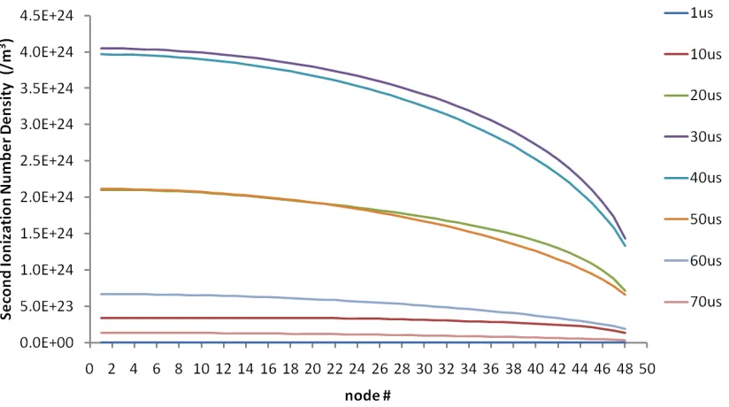
The ion number density of the second ionization N2, shown in Figure 4.13, peaks at

4.05 × 1024 /m3 in the first node in 30µs and drops to 1.33 × 1024 /m3 at the capillary exit; these values are 2 orders of magnitude less than that of the electron number density and the first ionization number density N1. The second ionization number density drops

(69)

Figure 4.13: Axial distribution of the second ionization state number density, N2, inside

the capillary at various times during the discharge.

The total number density of the plasma constituents in a partially ionized plasma includes the number density of the neutrals. Electrothermal plasmas are not fully ionized and so there will be a fraction of neutral particles in the plasma stream. Figure 4.14 shows the axial distribution of the neutral number density,N0, at various times of the discharge.

The neutral number density increases with time and peaks at 4.94 × 1026 /m3 in 70 µs and drops to 3.18 ×1026 _/m3 _{at the capillary exit.}

The total number density of the plasma, Np, is the sum of all number densities of

electrons Ne, ions (N1 and N2) and neutrals N0; and the axial distribution of the total

(70)

Figure 4.14: Axial distribution of plasma neutral number density,N0, inside the capillary

(71)

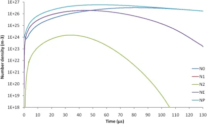
Figure 4.16: Time-dependent variation of the number densities at the capillary exit.

Figure 4.16 shows the variation of all number densities at the last node, where it is obvious that the electron and the first ionization number densities are almost the same and the second ion number density rises and peaks at 30µs then falls quickly, the neutral number density rises and stays unchanged at the end of the discharge, and the total number density also rises and stays unchanged till the end of the discharge.

(72)

(73)

(74)

4.2 Summary and Discussion of the Axial Behavior

of the Electrothermal Plasma Paremeters

(75)

Chapter 5 Effect of Extended Flat-Top Pulse

Length on the Plasma Parameters

5.1 Flat Top Pulses

(76)

Figure 5.1: Illustration of ideal interior ballistics profiles for electrothermal launchers.

(77)

Short pulses do not provide ideal ballistics, however, near ideal interior ballistic pro-files may be achieved by extending the discharge current to the shape and characteristics discussed in Chapter 4. Using these longer, flat-topped current pulses proved the neces-sary pressure to achieve the desired exit velocity.

In actual experiments, the plasma temperature will increase then decrease following the shape of the discharge current, similarly for the pressure. An extended flat-top discharge current would provide a near constant plasma pressure, a slow increase in plasma temperature, and an increasing velocity over the discharge period [55]. Chang and Howard reported that shorter pulse lengths, of about 300µs, are more powerful but provide less time for the interaction of the plasma flow with a solid target, and that plasma pulse length can have a strong influence on the flow characteristics. They also concluded that the pulse length is a key parameter that should be optimized for effective ignition, plasma propellant interactions, and electrothermal plasma propulsion systems [56].

Flat-top current pulses can be generated using a pulse forming network as shown in Figure 1.2, where the pulse is shaped via a combination of capacitors and inductors [55,57]. It is also possible to use high voltage high current crowbar switches, in which the discharge of a capacitor is shunted by a switch to extend the pulse [58,59]. Another technique to create long, flat pulses uses a homopolar generator which generates a high current DC voltage with the rotational motion of a magnet and a conductor [60]. Other systems may include high power DC energy storage systems such as a matrix of high current batteries to deliver the required discharge current to the capillary.

(78)

are important. These applications are those in which continuous, uniform output is necessary. While flattop pulse shape and amplitude can be experimentally generated by any of the above mentioned methods, these shapes can also be computationally generated for the purpose of electrothermal plasma code predictions.

A circuit module has been developed in the ETFLOW code to generate current pulses with the desired pulse length and amplitude. This model is based on a RLC circuit as shown in Figure 5.2, which represents the equivalent circuit of a capillary discharge [39]. The capacitorC0 represents the main source of energy storage, and the circuit inductance

(79)

circuit generates current pulses with the desired amplitude and pulse length by changing the voltage and the values of the circuit elements. The circuit module may be used with or without flattop extension to evaluate the behavior of the electrothermal source with various current amplitudes and pulse lengths. The module solves the seconds order RLC circuit:

L0

dI

dt +R0I =V0 −

Z _Idt

C0

(5.1)

From which the time rate of change of the current is given by:

dI

dt =

1

L0

V0−

Z _Idt

C0

−R0I

(5.2)

with the initial conditions I0=0, R

Idt= 0, and (dI/dt)=(V0/L0) at t=0. The time

increment is t = t + δ, whereδ is the time step, and the next step values are calculated by using the linear approximations:

I =I+dI

dtδ and

Z

Idt=

Z

Idt+δ (5.3)

(80)

Figure 5.3: Discharge current without flattop extension (zero extension) and with 100

µs extension.

(81)

Figure 5.4: Total ablated mass as a function of time for zero and 100 µs peak current extension for both ideal and nonideal model code results.

A summary of the total ablated mass as a function of the time extension up to 1000 µs is shown in Figure 5.5 for both the ideal and nonideal models. As shown in Figure 5.5, the total ablated mass increases almost linearly with the extension of the peak current over time, which is expected as a result of the continuous joule heating,

ηJ2_{, and the continuous ablation due to the radiation heat flux to the capillary wall}

(82)

Figure 5.5: Total ablated mass as a function of time extension for both ideal and nonideal models.

The total ablated mass for a 1000 µs flattop extension is 685.37 mg for the ideal plasma model and 492.12 mg when using the nonideal plasma model. These values, in both cases, are close to or more than a half gram of mass removed from the source. Typical masses of the Lexan sleeve prior to the discharge are about 5 g, thus the sleeve would survive 8-10 shots for a 1000 ms, 28.93 kA peak discharge current. The total ablated mass will differ depending on the sleeve material used in the capillary.

(83)

in Figure 5.6. Without flattop extension, the temperature peaks to 27,100 K (2.33eV) in 30µs for the ideal model and 25,000 K (2.15eV) for the nonideal model.

Figure 5.6: Plasma kinetic temperatures at the source exit as a function of time for zero and 100 µs peak current extension for both ideal and nonideal model code results.

(84)

total ablated mass of Figure 5.5, as the radiation heat flux is constant during the time extension,q” _∝_T4

plasma, and hence the rate of evaporation of the capillary wall continues

at a constant rate. A summary of the peak plasma temperature at the source exit as a function of the time extension up to 1000µs is shown in Figure 5.7 for both the ideal and nonideal models. As seen from the figure, the peak plasma temperature stays constant at 27,100 K (2.33eV) for the ideal model and 25,000 K (2.15eV) for the nonideal model.

(85)

The plasma pressures at the source exit as a function of time for zero and 100 µs extension for both ideal and nonideal model code results are shown in Figure 5.8. Without extension the pressure peaks at 228 MPa for the ideal model and 156 MPa for the nonideal model in 50 µs and immediately drops at a fast rate.

Figure 5.8: Plasma pressure at the source exit as a function of time for zero and 100 µs peak current extension for both ideal and nonideal model code results.

For the 100 µs extension of the pulse the pressure increases above 250MPa in 60

(86)

shown in Figure 5.1. The peak pressure as a function of the extension time is plotted in Figure 5.9, where it is obvious that the pressure increases with increasing extension

Figure 5.9: Peak plasma kinetic temperatures at the source exit as a function of the time extension of the peak discharge current for both the ideal and nonideal models.

time until 100 µs and remains unchanged for further extensions up to 1000 µs. Because the pressure is determined by the temperature and the number density of the plasma constituents, ρ=P

(87)

(88)

The plasma bulk velocity at the source exit as a function of time for zero and 100

µs peak current extension for both ideal and nonideal model code results are shown in Figure 5.11. Without extension of the current peak, the bulk velocity peaks at 5.72 km/s for the ideal model and 5.44 km/s for the nonideal model in 30 µs then drops at a faster rate for the rest of the pulse.

Figure 5.11: Plasma bulk velocities at the source exit as a function of time for zero and 100 µs peak current extension for both ideal and nonideal model code results.

(89)

function of the extension time is plotted in Figure 5.12, where it is clear that the exit velocity for a 28.93 kA peak discharge current is greater than 5 km/s (for calculations with ideal and nonideal models) and remains constant for all tested extension periods. Thus, achieving a constant exit bulk velocity for longer discharge periods is possible with extended flattop current pulses, which is useful in space thruster applications.

Figure 5.12: Peak plasma bulk velocities at the source exit as a function of the time extension of the peak discharge current for both the ideal and nonideal models.

(90)

(91)

5.2 Summary and Discussion of the ETFLOW Code

for Flattop Pulse Modeling

The electrothermal code ETFLOW has been used to calculate the plasma parameters for extended flattop peaks of the discharge current to explore the feasibility of such sources for applications with near ideal interior ballistics. A circuit module was built in the code to generate current pulses with desired shapes and amplitudes. The discharge current for an actual shot (shot P228, 28.93 kA peak with initial pulse length of 100

A Numerical Study of the Non-Ideal Behavior, Parameters, and Novel Applications of an Electrothermal Plasma Source.

Abstract

Dedication

Biography

Acknowledgements

Table of Contents

List of Tables

List of Figures

Chapter 1

Introduction

1.1

Electrothermal Plasma Background

1.2

The Electrothermal Plasma Source

1.3

Motivation and Goals of the Study

Chapter 2

Governing Equations of the Model

and the ETFLOW Code

2.1

Basic Assumptions of the Plasma Model

2.2

Conservation of Mass

2.3

Conservation of Momentum

2.4

Conservation of Energy

Chapter 3

The Effect of a Non-Ideal Plasma

Model on the Electrothermal

Plasma Parameters

3.1

Non-Ideal Effects on Physical Parameters

3.2

Non-Ideal Effects on Electrical Conductivity

3.3

Summary of the Inclusion of the Non-Ideal Model

in the ETFLOW Code

Chapter 4

Axial Behavior of the Plasma

Parameters

4.1

A Case Study of the Axial Plasma Parameters

of Shot P228

4.2

Summary and Discussion of the Axial Behavior

of the Electrothermal Plasma Paremeters

Chapter 5

Effect of Extended Flat-Top Pulse

Length on the Plasma Parameters

5.1

Flat Top Pulses

5.2

Summary and Discussion of the ETFLOW Code

for Flattop Pulse Modeling