Bayesian Variable Selection for Detecting Adaptive Genomic Differences Among Populations

DOI: 10.1534/genetics.107.081281

Bayesian Variable Selection for Detecting Adaptive

Genomic Differences Among Populations

Andrea Riebler,*

,1

_{Leonhard Held* and Wolfgang Stephan}

†

*Biostatistics Unit, Institute of Social and Preventive Medicine, University of Zurich, CH-8001 Zurich, Switzerland and†Section of Evolutionary Biology, Department of Biology II,

University of Munich, D-82152 Planegg-Martinsried, Germany Manuscript received August 29, 2007

Accepted for publication December 26, 2007

ABSTRACT

We extend anFst-based Bayesian hierarchical model, implemented via Markov chain Monte Carlo, for the detection of loci that might be subject to positive selection. This model divides theFst-influencing factors into locus-specific effects, population-specific effects, and effects that are specific for the locus in combination with the population. We introduce a Bayesian auxiliary variable for each locus effect to automatically select nonneutral locus effects. As a by-product, the efficiency of the original approach is improved by using a reparameterization of the model. The statistical power of the extended algorithm is assessed with simulated data sets from a Wright–Fisher model with migration. We find that the inclusion of model selection suggests a clear improvement in discrimination as measured by the area under the receiver operating characteristic (ROC) curve. Additionally, we illustrate and discuss the quality of the newly developed method on the basis of an allozyme data set of the fruit flyDrosophila melanogasterand a sequence data set of the wild tomatoSolanum chilense. For data sets with small sample sizes, high mutation rates, and/or long sequences, however, methods based on nucleotide statistics should be preferred.

L

IKE many biologists, we are interested in the ques-tion of how animals and plants adapt to changes in their environment. Which regions in the genome are responsible for adaptation after climate catastrophes or the use of environmental toxins? There is growing interest in developing methods to detect loci that might be subject to selection (see Glinkaet al.2003; Ronald and Akey2005; Vasema¨ giet al.2005; Boninet al.2006; Li and Stephan2006; Mealorand Hild2006), as these loci might be functionally important (Beaumont and Balding2004).

Individuals from different subpopulations living in different environments often vary genetically at a few key sites in their genome due to the adaptation to different local conditions. The amount of genetic differentiation can be measured from differences in allele frequencies among different populations, summarized by an esti-mate of theFst-coefficient first introduced by Wright (1943). Low Fst-values may indicate balancing selec-tion, whereas highFst-values suggest positive directional selection.

Beaumontand Nichols(1996) developed a method, called FDIST, which starts with the calculation ofu, an estimator of the Fst-coefficient, for each locus in the sample. Then coalescent simulations are performed to generate data sets with a distribution ofusimilar to the

empirical distribution, from which P-values and quan-tiles are calculated. The quanquan-tiles of this distribution are compared with the obtainedFst-values to classify loci as selected or neutral. Simulation studies showed that this method detects at an acceptable rate loci subject to positive directional selection but lacks power to detect balancing selection (Beaumont and Balding 2004). Beaumontand Balding(2004) developed a likelihood-based approach, implemented via Markov chain Monte Carlo (MCMC), which uses a Bayesian hierarchical model similar to that of Balding(2003). In this model, each individual Fst-value for a particular population and a particular locus integrates effects that are specific to the given locus, effects that are specific to the given pop-ulation, and effects that are specific to both the locus and the population (Beaumont and Balding 2004). Applications to simulated data sets with predominantly neutral loci but with some loci subject to directional or balancing selection suggested that the Bayesian method of Beaumontand Balding(2004) performed slightly better than FDIST and seemed also to detect loci subject to balancing selection. However, ideally we want to test, within a Bayesian framework, the hypothesis of whether a locus is subject to selection (Beaumontand Balding 2004). To avoid the problem of specifying appropriate alternative hypotheses we introduce an auxiliary variable for each locus effect to automatically select nonneutrally behaving locus effects. The idea to include Bayesian model selection was already considered by Beaumont and Balding(2004) but not further elaborated.

1_{Corresponding author:Biostatistics Unit, Institute of Social and}

Pre-ventive Medicine, University of Zurich, Hirschengraben 84, CH-8001 Zurich, Switzerland. E-mail: [email protected]

In this article, we extend the Beaumontand Balding (2004) approach. A new Bayesian auxiliary variable is introduced for each locus effect (Dellaportas et al. 2002). The new variable indicates whether a specific locus can be regarded as selected and therefore the locus effect has to be included in the model, or it can be regarded as neutral. By looking at the posterior distri-bution of the auxiliary variable it is possible to infer whether the locus is subject to selection. Through the prior distribution, the approach deals with the problem of multiple testing. As a prior distribution for the auxiliary variables we assume independent and identical Bernoulli distributions with parameterp, where p isa priori beta distributed. The (hyper)parameters of the beta distribution are specified in the way that only a small fraction of loci (10%) area prioriexpected to be under selection. As a by-product, the efficiency of the algorithm is increased by a reparameterization, so that Gibbs sampling can be used. The method is applied to simulated data sets from a Wright–Fisher model with migration and with some loci subject to balancing or positive directional selection and to real data sets.

MATERIALS AND METHODS

Hierarchical Bayesian method: Model: Beaumont and

Balding (2004) developed a hierarchical Bayesian model,

implemented via MCMC, to distinguish loci subject to selec-tion from neutral loci. The model has two levels: a lower-level model, in which the likelihood for the allele-frequency counts is expressed as a function ofFst, and a higher-level model for theFst-values. Allele-frequency counts at a locus within a pop-ulation are modeled using the multinomial Dirichlet likeli-hood. This likelihood arises in a simple migration–drift model; for derivations see Baldingand Nichols(1995) and Balding

(2003). The multinomial-Dirichlet likelihood can be conve-niently expressed in the form

Lij ¼Pðaij1;. . .;aijKijlij;xi1;. . .;xiKiÞ

¼ GðlijÞ Gðnij1lijÞ

YKi

k¼1

Gðaijk1lijxikÞ

GðlijxikÞ

; ð1Þ

whereaijk, withi¼1,. . .,I(Iis the number of loci),j¼1,. . .,J (Jis the number of populations), andk¼1,. . .,Ki(Kiis the number of alleles at locusi), denotes the count of allelekin populationjat locusi,nij ¼

PKi

k¼1aijkdenotes the sample size, andxikis the frequency of allelekat locusiin the migrant gene pool. The scaling parameterlijis defined as

lij ¼

1 Fstij

1:

As the allele-frequency counts corresponding to distinct loci and different subpopulations are assumed to be mutually in-dependent, the joint likelihood is given by

L¼Y

I

i¼1 YJ j¼1

Lij:

The precision of the estimates is improved when information aboutFstijis shared across loci and subpopulations by

employ-ing a hierarchical model. EachFstijcan be seen as a combination of contributions from locus-specific effects, such as mutations and some forms of selection, and population-specific effects, such as effective population size, migration rates, and popula-tion-specific mating patterns. These effects are included using a regression approach. Beaumontand Balding(2004) chose

the logistic regression model

log 1 lij

¼log F

ij

st 1Fstij

¼ai1bj1gij;

or equivalently

Fij

st ¼

expðai1bj1gijÞ

11expðai1bj1gijÞ

;

where aiis a locus effect,bja population effect, andgij an interaction term representing a specific locus-by-population effect. The averageFst-value for a particular locusiis obtained by using its locus effect, the average over the population ef-fects, and the average of the corresponding interaction effects with each population (M. A. Beaumont, personal

communi-cation). Gaussian priors f, as defined in Beaumont and

Balding(2004), are used for the regression parametersai,

bj, andgij. The means and variances were selected in the way that the implied prior distribution for each Fstij has non-negligible density over almost the whole interval from zero to one. Forxi, a (multivariate) uniform distribution is chosen as a prior distribution.

Further method development: For determining loci that might be subject to selection, the primary interest is directed toward the posterior distribution of the locus effects. A high positive value ofaisuggests that locusimight be subject to positive directional selection, whereas a negative value indi-cates balancing selection. Ideally, we want to assign a posterior probability to each hypothesis of the formai¼0. In this way, the posterior probability indicates whether a locusiis neutral and hence has a zero locus effect or is subject to selection. To avoid the specification of alternative hypotheses, we use a reparameterization and introduce an additional Bernoulli-distributed auxiliary variable di to indicate whether locus i might be subject to selection (Holmesand Held2006). This

approach also deals with the problem of multiple testing of many genomic locations, as the number of tested loci is taken into account through the prior distribution of the auxiliary variables.

Reparameterization: The original framework used the varia-blesai,bj,gij, andxi. Now, a new variablehijis introduced,

h_ij ¼ai1bj1gij¼log

Fij

st 1Fstij

; ð2Þ

which creates a new layer in the definition ofFstij, as now theF ij st -value only depends onhijdirectly, andhijdepends onaiand bj. Thegijvalues are no longer sampled but thehijvalues are. Of course, thegijvalues can be recalculated on the basis ofhij, ai, andbj. The implied prior distribution ofhijjai,bjis given by

h_ijja_i;b_j Nðai1bj1mg;s2hÞ

for i¼1;. . .;I and j ¼1;. . .;J;

wheremgis the prior mean ofgands2his the prior variance of g. The prior distributions foraiandbjremain unchanged.

Introduction of Gibbs variable selection: To indicate whether locusimight be neutral, or subject to selection, Gibbs variable selection was applied (for a recent review see Dellaportas

withi¼1,. . .,Iwere included in the model specification, so that

h_ij¼diai1bj1gij:

The indicator vector d shows which of theI possible locus effects are present in the model and, therefore, are assumed to be nonneutral. From the posterior distribution of thediit is possible to infer whether a locus is subject to selection. The prior distribution ofhijchanges to

h_ijjai;di;bj Nðdiai1bj1mg;s2hÞ:

It would be also possible to exclude the corresponding locus-by-population effect if a locus is considered as neutral. However, we decided to keep this interaction term as it might indicate a selective pressure that is present just for a specific population at this locus.

As a prior distribution fordiwithi¼1,. . .,I, we assume dijpBernoulliðpÞ independently andpBeð0:2;1:8Þ. We selected the hyperparameters of the beta distribution to achieve a nonnegligible density over the whole interval from zero to one and a biologically realistic prior expectation of the number of loci subject to selection. Using the law of iterated expectations, it follows that

EðdiÞ ¼EðEðdijpÞÞ ¼EðpÞ ¼0:1:

The prior distribution for the locus effects changes toai N(0, 10), as

VarðdiaiÞ ¼Eðd2i a2iÞ ½EðdiaiÞ2

¼Eðdia2iÞ ¼EðdiÞEða2iÞ

¼0:1s2a;

so that the variance of 1 is ensured, as used in Beaumontand

Balding(2004).

Implementation: The goal is to obtain values from the pos-terior distribution (proportional to the product of the likelihood and the prior distributions), which, for the original algorithm, takes the form

fða;b;g;xjaÞ}Pðaja;b;g;xÞ |fflfflfflfflfflfflfflfflfflfflffl{zfflfflfflfflfflfflfflfflfflfflffl}

L¼QI

i¼1

QJ j¼1Lij

fðaÞfðbÞfðgÞfðxÞ:

(Here, the prior distributions for a, b, g, and x are in-dependent.) This is achieved by MCMC on the basis of iteratively updating the corresponding conditional distribu-tions (full conditionals) (Besag_{et al.}1995). The estimation

procedure is implemented as a Metropolis–Hastings Monte Carlo algorithm. At each step, the algorithm proposes a Gaussian update for eachai, eachbj, and eachgij, using the corresponding current parameter value as the mean. The variances can be chosen arbitrarily, but the choice can be optimized for achieving fast convergence. Ideally, the varian-ces should be adapted to achieve acceptance rates between 25 and 45% (Gelmanet al.1996). Here, the variance fora

iis initialized with 1.22_{, the variance for b}

j with 0.62, and the variance forgijwith 1.42. If the acceptance rates are not within the desired interval after the burn-in iterations, the variances are adapted by the addition or the subtraction of 0.1 (if the variances are,0.1 only 0.01 is subtracted) and the chain is restarted. Since the normal distribution is symmetric around the mean, the update is accepted or rejected as in the Metrop-olis algorithm. The frequencies xi¼ ðxi1;. . .;xiKiÞ are also

updated, one locus at a time. The proposed value is chosen

from a Dirichlet distribution with the mean proportional to the current values

x*ijxiDirðcixi1;. . .;cixiKiÞ;

where theciare locus-dependent constants used to adapt the acceptance rates. To initialize the constantscidependent on Kia simple regression function is used. In the case that the acceptance rates are not between 25 and 45% after the burn-in iterations, the constantsciare increased or decreased by 2% for every percentage of deviation from a target acceptance rate of 35% and the burn-in interval is repeated. When using a Dirichlet distribution as a proposal distribution the frequen-ciesxikcan become very small. To avoid this, a minimum allele frequency of 103_{is used. Since the Dirichlet distribution is not} symmetric, a Metropolis–Hastings update is required for xi (Beaumontand Balding2004).

As a consequence of introducing hij, the full conditional distributions ofaiandbjare normal distributions, so that it is now possible to sample directly from them, since

fðaija;ai;b;h;xÞ}fðaiÞ

YJ j¼1

fðh_ijjai;bjÞ;

where

ai¼ ða1;. . .;ai1;ai11;. . .;aIÞ:

Hence

aijNðmaj;s 2 ajÞ

with

s2 aj¼

1 s2a

1 J

s2h !1

;

maj¼ 1 s2a

1 J

s2h !1

ma

s2a

1 1

s2h

X

J

j¼1

ðh_ijb_jmgÞ !

:

For the derivation of s2

aj and maj see,e.g., Bernardo and

Smith(1994, p. 439). Analogously, we haveb

jN(mbj,s

2 bj)

with

s2_bj¼ 1 s2b

1 I

s2h !1

;

mbj¼ 1 s2 b

1 I

s2 h

!1

mb

s2 b

1 1

s2 h

X

I

i¼1

ðh_ijaimgÞ !

:

For thehijthe full conditional distribution

fðh_ijja;a;b;xÞ}fðh_ijjai;bjÞ Lij

is obtained, withLijdefined as a multinomial Dirichlet likeli-hood as in Equation 1. For updating the hij a random-walk proposal

h*

ijjhij Nðhijjs2h*Þ

is used, where s2

h*is initialized with 1.4

2_{and adapted as} de-scribed above forai,bj, andgijto reach acceptance rates be-tween 25 and 45%. The update is accepted as in the Metropolis algorithm.

distributions. This method is also known as Gibbs sampling (Gilkset al.1996). One potential problem might be that the

posterior correlation betweenhijandai,bj(see Equation 2) might cause slow mixing and, therefore, slow convergence (Holmesand Held2006). To illustrate the relative efficiency

change of the reparameterization over the original method, the total CPU run time was recorded for both methods and the ‘‘effective sample size’’ (ESS) calculated. ESS is an estimate of the number of independent samples that would be required to obtain a parameter estimate with the same precision as the MCMC estimate based onNdependent samples (hereN ¼ 10,000). ESS can be interpreted as a measure of the in-formation content of the MCMC samples. An ESS value close toNindicates that the MCMC samples are virtually uncorre-lated. The effective sample size is calculated as the number of MCMC samples drawn divided by the autocorrelation timet, which is defined as

t¼112X

‘

s¼1

rðsÞ so that ESS¼N

t; ð3Þ

wherer(s) is the autocorrelation at lag sand measures the degree of association between sampled values of the moni-tored Markov chain separated by lags. As the real autocorre-lations are estimated by the sample autocorreautocorre-lations, it is necessary to cut off the estimation oftat ans-valuevwhere the autocorrelations are sufficiently close to zero. The inclusion of estimates for much higher lags would add too much noise (Kass et al. 1998). The cutoff value v is determined using

the initial monotone sequence estimator (IMSE) by Geyer

(1992). Define

FðsÞ ¼rð2sÞ1rð2s11Þ

and letrbe the largest integer such thatF(s).0 andF(s) is monotone fors¼1,. . .,r; thenvis defined asv¼2r11 (Geyer1992).

Introducing the auxiliary variabledi, the updates ofbjand hijare unchanged butaiis substituted bydiai. Ifdi¼1 the update ofaialso stays unchanged. In contrast,aiis sampled from its prior distribution ifdi¼0. Each elementdiis thereby updated as part of the algorithm. The full conditional dis-tribution ofdiis given by

fðdija;a;di;b;h;x;pÞ}fðdijpÞ

YJ j¼1

fðh_ijjai;di;bjÞ;

whereby the parameter p is updated every iteration by sampling from its full conditional distribution

pjd1;. . .;dI Be 0:21

XI i¼1

fdi¼1g;1:81

XI i¼1

fdi¼0g

! :

Interpretation: In the original setting by Beaumont and

Balding(2004), a posterior distribution fora_iis classified as

significantly positive and therefore subject to positive direc-tional selection if its 5% quantile is positive or equivalently if P(ai,0jdata)#0.05. It is classified as significantly negative and therefore subject to balancing selection if its 95% quantile is negative or equivalently ifP(ai,0jdata)$0.95. In the following, the posterior probabilityP(ai ,0 jdata) is also referred to as a BayesianP-value.

Using Gibbs variable selection the posterior probabilities P(di¼1jdata) instead of the BayesianP-values are used to detect significant loci. In this way, a locusiis classified as being subject to selection ifP(di¼ 1jdata) is greater than some cutoff value that will be set by means of the simulation study results. To classify a nonneutral locus subject to positive di-rectional or balancing selection we use the Fst-value at the smallest observed posterior probabilityP(di¼1jdata) as a threshold. Selected loci with a smallerFst-value are classified as subject to balancing selection, and those that have a largerF st-value are classified as subject to positive directional selection. In the context of selection, the locus-by-population effects gijmight also be important. For example, a large positive value of gij might indicate a population in which local positive selection has driven an allele to fixation whereas this selection pressure can be weak or absent for that locus in the other populations. As the full conditional distribution ofgijdoes not combine information across loci or populations, only ex-tremely large selective influences can be found by inspecting thegijvalues (Beaumontand Balding2004).

Simulation study:To compare the behavior of the different methods and to assess their performance in detecting non-neutrally behaving loci we simulated gene-frequency data from a Wright–Fisher model with migration, which is similar to that of Beaumontand Balding(2004). In our simulations,

all populations are assumed to have the same size,N¼10,000 chromosomes. Chromosomes in the current generation are replaced with immigrants. The immigration rate is defined by m¼ ð1FÞ=2NF, whereby the value of F is either set to a fixed value (e.g., 0.2) or sampled from a beta distribution, with parameters 0.25 and 2.25 as given in Beaumontand Balding TABLE 1

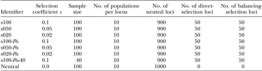
Parameter values of the data sets simulated from the Wright–Fisher model with migration

Identifier

Selection coefficients

Sample size

No. of populations per locus

No. of neutral loci

No. of direct-selection loci

No. of balancing-selection loci

s100 0.1 100 10 900 50 50

s050 0.05 100 10 900 50 50

s020 0.02 100 10 900 50 50

s100-Fb 0.1 100 10 900 50 50

s050-Fb 0.05 100 10 900 50 50

s020-Fb 0.02 100 10 900 50 50

s100-Fb-40 0.1 40 10 900 50 50

Neutral 0.0 100 10 1000 0 0

(2004), to allow variable immigration rates over the popula-tions. Then the next generation is sampled according to a specified selection coefficients. The algorithm is repeated for Tgenerations. In all analyses, we used 1000 generations, which should not lead to any equilibrium, but should reflect the selection coefficient. A selective sweep is assumed to take ð4logð2NÞÞ=sgenerations. Assuming the advantage of a selected allele to bes/2, which is described in more detail in

appendix a, the choice ofTshould be sufficiently large for a

selection coefficient of 0.1. For selection coefficients that are >0.1 we expect the results to be worse. To allow for adaptive selection the attributes ‘‘neutral,’’ ‘‘red,’’ or ‘‘blue’’ are as-signed at random and independently to the populations. The consequence is that the number of populations for which a selective pressure exists at a locus under selection is random. In neutral populations all alleles have the same fitness. After 1000 generations, a specified number of chromosomes is sampled with replacement to represent the allele frequencies for the given locus and population. The model is repeated for all populations and all loci to get a complete simulated data set, where we used within a data set the same selection coef-ficient for loci subject to balancing and positive directional selection. A detailed description of the simulation study de-sign is given inappendix a.

We generated eight data sets, each of which consists of 1000 loci and 10 populations per locus to systematically test the power of the different methods. Focus was set on the influence of different selection coefficients but also on the influence of sample size and migration rate. The details and properties of the different data sets are given in Table 1.

Real data sets:As in Beaumontand Balding(2004), the

Drosophila melanogasterallozyme data set of Singhand R hom-berg(1987) was analyzed. The allele-frequency table for this

data set is provided with the program FDIST 2 (http:// www.rubic.rdg.ac.uk/mab/software/fdist2.zip) and includes allele counts for 61 polymorphic loci in 15 geographically distant populations ofD. melanogaster. The considered popula-tions as given in the allele-frequency table are as follows: Ottawa, Canada (OTT) (80 iso-female lines); Hamilton, Ontario, Canada (HAM) (161); Amherst, Massachusetts (MAS) (121); Brownsville, Texas (TEX) (121); La Plata, Argentina (ARG) (38); Sweden (SWE) (40); Ukraine (UKR) (44); Central Asia (CAS) (40); France (FRA) (81); Benin, West Africa (WAF) (114); Central Africa (CAF) (68); Seoul, Korea (KOR) (132); Taiwan (TAI) (80); Ho-Chi-Minh City, Vietnam (VIE) (80); and Fairfield, Australia (AUS) (100). The loci are mostly di- or triallelic. The maximum number of alleles for a locus is nine (Singhand Rhomberg1987).

Figure1.—ROC curves of three simulated data sets analyzed with the reparameterized method without Bayesian variable

se-lection and with Bayesian variable sese-lection. The power, also known as the true positive rate, is plotted against the false positive rate. Similar ROC curves are obtained for the other simulated data sets.

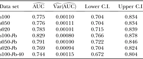
TABLE 2

ROC analysis of the simulation results for the method without Bayesian variable selection

Data set AUCb VardðAUCbÞ Lower C.I. Upper C.I.

s100 0.775 0.00110 0.704 0.834

s050 0.776 0.00111 0.704 0.834

s020 0.783 0.00101 0.715 0.839

s100-Fb 0.829 0.00080 0.766 0.878 s050-Fb 0.791 0.00100 0.722 0.846 s020-Fb 0.769 0.00094 0.704 0.824 s100-Fb-40 0.744 0.00115 0.672 0.804

Estimated AUC values, the empirical variance of AUC, and estimated 95% confidence intervals are shown.

TABLE 3

ROC analysis of the simulation results for the method with Bayesian variable selection

Data set AUCb dVarðAUCbÞ Lower C.I. Upper C.I.

s100 0.895 0.00026 0.859 0.923

s050 0.896 0.00025 0.860 0.923

s020 0.898 0.00026 0.861 0.925

s100-Fb 0.917 0.00019 0.885 0.941 s050-Fb 0.900 0.00025 0.864 0.927 s020-Fb 0.887 0.00025 0.852 0.914 s100-Fb-40 0.848 0.00044 0.802 0.884

The second data set was published by Arunyawat et al.

(2007) and contains sequences of the wild tomato species Solanum chilensedistributed from northern Chile to southern Peru. The data set includes four different populations: Antofagasta, Chile; Tacna, Peru; Moquegua, Peru; and Qui-cacha, Peru. For this data set, eight loci were examined: CT066, CT093, CT166, CT179, CT198, CT208, CT251, and CT268. There were five to seven (diploid) individuals for each population, leading to 2 sequences from each individual for each locus. Therefore, the sample size is 10–14 sequences. The total length of individual loci (including indels) ranges from 778 to 1887 bp. An allele-frequency table was calculated treating each distinct haplotype at a locus as a new allele. The numbers of haplotypes for the loci vary between 23 and 30.

Environment details:All analyses were run on an Intel Core 2 Duo T7200 processor with 1024 MB DDR-2-RAM under Kubuntu 7.04 (Feisty Fawn). Each algorithm was run to obtain 10,000 output samples for each variable. In the case of the real data sets the algorithm was run for 1,000,000 post burn-in iterations using a thinning interval ofk¼100. For the 1000-locus simulations we used 250,000 post burn-in iterations and a thinning interval ofk¼25. To check convergence standard diagnostic tests were applied. The analysis of the 1000-locus simulation described in Table 1 took9 hr.

The executable C-files of the different algorithms used in this study are available on request from A. Riebler. Additional R programs to visualize and analyze the results as well as the data sets used in this study are also available. All programs were developed under SuSE Linux 10.0 and Kubuntu 7.04 (Feisty Fawn).

RESULTS

Simulation study results: We used simulation studies

to discuss the quality of the different methods in detecting loci subject to selection and to determine a suitable cutoff value for the reparameterized method with variable selection. For these purposes seven simu-lated data sets with predominantly neutral loci but with some loci subject to balancing or positive directional selection and one neutral data set were generated (see Table 1). The reparameterized method without variable selection is expected to increase the efficiency of the original method by Beaumont and Balding (2004),

which will be confirmed by the application to the D. melanogasterdata of Singhand Rhomberg(1987). Since this method is only a reformulation, the original method is not used in this simulation study. The power of the methods was assessed by a receiver operating character-istic (ROC) analysis. For detailed descriptions, compare appendix b. We generated ROC curves for all seven (nonneutral) simulated data sets. A ROC curve is a graphical plot of the power vs. (1 specificity) for a binary classification system whereby the cutoff value is varied. In this analysis we did not distinguish between loci subject to balancing and directional selection. For all simulations we got very similar ROC plots, three of which are shown in Figure 1. It is obvious that the ROC curve of the method with variable selection is nearly always above the ROC curve of the method without Bayesian variable selection. We also tried a uniform prior distribution for the probability of including a locus effect that resulted in similar ROC curves. To measure the quality of the different methods the area under the ROC curve (AUC) was used. A perfect ROC curve has the value AUC¼1.0. In contrast, an uninformative test has AUC ¼0.5 (Pepe 2003). The AUC values and the corresponding 95% confidence intervals are shown in Table 2 for the method without Bayesian variable selection and in Table 3 for the method with Bayesian variable selection. Since the scale for the AUC is re-stricted to (0, 1), the confidence intervals were calcu-lated on the logit scale (Pepe 2003). To compare the empirical ROC curves we used the difference in esti-mated AUC values (seeappendix b). The null hypoth-esis that the AUC value of the method with variable selection is not higher than the AUC value of the method without variable selection is tested by compar-ing the value ofDAUC=seb ðDAUCbÞwith the 99% quantile (2.326) of a standard normal distribution (Pepe2003). The obtained test statistics are shown in Table 4. In all cases the values of the test statistic are much larger, so the null hypothesis was rejected. This means the AUC was sig-nificantly higher for the new Bayesian variable approach.

TABLE 4

Comparison of the empirical ROC curves

Data set DbAUC VardðDbAUCÞ Lower C.I. Upper C.I. DbAUC=seðDbAUCÞ

s100 0.119 0.00033 0.084 0.155 6.541

s050 0.120 0.00035 0.083 0.157 6.403

s020 0.114 0.00028 0.081 0.147 6.760

s100-Fb 0.088 0.00024 0.058 0.119 5.730

s050-Fb 0.109 0.00029 0.075 0.142 6.338

s020-Fb 0.118 0.00028 0.085 0.151 7.079

s100-Fb-40 0.104 0.00022 0.075 0.134 7.046

The predictions are reasonably well calibrated; for example, predictions with 10% probability occur 7– 8% of the time with a lower 95%-confidence limit be-tween 5 and 6% and an upper 95%-confidence limit between 9 and 11%. Predictions with 5% probability occur5–6% of the time with a lower 95%-confidence limit between 3 and 4% and an upper 95%-confidence limit between 6 and 7%.

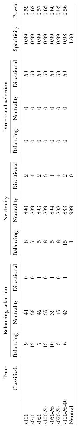
By means of the results of the simulation studies we determined a threshold value for the reparameterized method with variable selection of 0.17 for classifying a locus as being subject to selection. We decided thereby to control the false positive rate and used the threshold value that achieved a specificity of at least 98% in all simulated data sets.A priorithe probability for a value

.0.17 is 20%. The results of the application to the simulated data sets are shown in Table 5. In comparison the results for the method without Bayesian variable selection, which uses the classification criterion de-scribed in the previous section, are shown in Table 6.

Both methods classified all loci subject to directional selection correctly. The method without variable selec-tion detected more loci subject to balancing selecselec-tion but also had a much higher false positive rate. Of the 7300 neutral loci in all eight data sets, 464 loci (6.36%) were misclassified as subject to balancing selection and 87 loci (1.19%) as subject to directional selection. For the method with variable selection, the rates were 0.78% for balancing false positives and 0.25% for directional false positives. In the case of the neutral simulated data set the method with variable selection classified all ex-cept one locus correctly. In contrast, the method without variable selection misclassified 20 neutral loci as subject to balancing selection and 39 loci as subject to positive directional selection. For both methods we found that a reduction of the sample size from 100 to 40 leads to a reduction of power. Choosing the immigration rate to be variable has no clear effect. However, in the case of the method without variable selection the rate of false positives clearly increased, while a specificity of 0.99 was maintained for the method with variable selection. With variable migration rate the influence of the se-lection coefficient became more apparent. At higher selection coefficients more loci subject to balancing selection were detected.

Example data sets: We first reanalyzed the D.

mela-nogasterdata of Singhand Rhomberg(1987).

Comparison of the results of B

eaumont

and B

alding

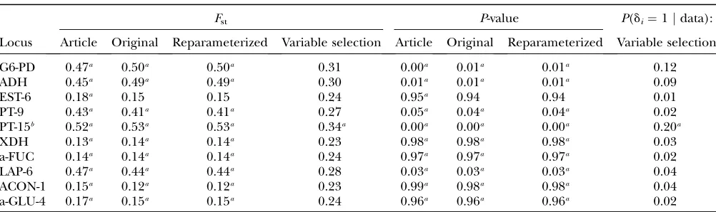
(2004) and the original reimplemented algorithm:Beaumont and Balding(2004) identified 10 loci as being subject to selection. The newly implemented version detected 9 of these 10 loci. The locus EST-6 was not detected as being subject to balancing selection, but its Bayesian

P-value is close to the critical value (see Table 7). All BayesianP-values obtained are nearly identical to those obtained by Beaumont and Balding (2004), whereas theFst-values show small differences (compare Table 7).

Table 7 and Figure 2 show that the results of Beaumont and Balding (2004) could be reproduced, except for small deviations, indicating that the newly implemented version is correct.

Comparison of the original and the reparameterized version:

The results of the reparameterized method are identi-cal to those of the original model (see Table 7). This re-sult was expected, because the reparameterization does not entail any changes to the algorithm. It is only a re-formulation that increases efficiency by allowing us to sample directly from the full conditional distributions of a_iandb_j.

Efficiency:The effective sample size ESS was calculated for all locus effectsa_iand then averaged; analogously the ESS was calculated for the population effectsbj. Table 8

shows the results, with the last column presenting the relative efficiency of the reparameterized method over the original method, indicated by the relative effective sample size standardized for CPU run time. As expected, the reparameterization caused higher autocorrelations in the chain but led to an improvement in the standard-ized relative ESS. Considering this efficiency gain, the reparameterized version should be preferred. There-fore the original version was not considered further.

Results of the reparameterized method including Bayesian variable selection: The results for the reparameterized method with variable selection are shown in Figure 2. Instead of the BayesianP-values the posterior probabil-itiesP(di¼1jdata) were used to detect significant loci.

The cutoff value is 0.17 as determined in the previous simulation studies.

Accuracy: One of the 10 loci identified by Beaumont and Balding (2004) was detected as being subject to selection by the new method with Bayesian variable selection. No additional loci were considered signifi-cant. Beaumontand Balding(2004) showed by simu-lations that very few loci being subject to balancing selection were identified by their Bayesian hierarchical method, but if loci were classified as being subject to balancing selection, the identification was mostly cor-rect. Beaumontand Balding(2004) detected 5 loci as being subject to balancing selection. However, none of these loci were inferred as being subject to balancing selection by the method with Bayesian variable selection.

Locus-by-population effects:In accordance with Beaumont and Balding (2004) all methods found an extremely highgij value for the biallelic locus PT-26 in the West

African sample and a significantly negativegijvalue for

locus AO in the sample from Texas.

The highest posterior expectation E(ai 1 gij) was

found for the triallelic locus G6-PD. In the sample from Texas, the allele that is the rarest in 13 of the other 14 populations is fixed. The reason could be a selec-tive pressure at this locus that is absent in the other populations.

Analysis of tomato data: As a second example, we analyzed the sequence data set from S. chilense. This

data set includes large DNA regions, and nearly every haplotype represents a new allele;e.g., the number of unique haplotypes is high. Figure 3 shows that there were no locus effects classified as significant. All F st-values are very close to zero, indicating that there are no signatures of directional selection in the data. However, as all Fst-values are small, it seems probable that the haplotype counts contained too little information about genetic differentiation.

Accuracy:This tomato data set is a typical extreme data set in the sense of Hudsonet al.(1992a). Arunyawat et al.(2007) estimated parameters of genetic differenti-ation with the program DnaSP version 4.0 (Rozaset al. 2003), which, in addition to haplotype-based methods, used nucleotide-based methods. The nucleotide-based statistics by Hudson et al. (1992b) obtained clearly higher values than the haplotype-based ones. For ex-ample, for locus CT208, an Fst-value of 0.340 was ob-tained (compare Arunyawatet al.2007, Table 4). This value indicates positive directional selection, whereas the value obtained by the methods developed here hints toward balancing selection as a more likely alternative. The haplotype-based statistics by Nei (1973) used in DnaSP also yielded smaller values than the nucleotide-based statistics.

DISCUSSION

Many previous studies have used BayesianP-values to identify loci subject to selection (e.g., Beaumont and Nichols1996; Beaumont and Balding2004). Here, we presented two extensions of an algorithm developed by Beaumont and Balding (2004) to automatically select nonneutrally behaving loci by introducing

Bayes-ian variable selection. First, we reparameterized the model framework and showed that this increases the efficiency. Then we introduced a new Bayesian auxiliary variable to decide whether a locus is subject to selection. We applied the reparameterized method with and without Bayesian variable selection to a fruit fly allozyme data set, to a wild tomato sequence data set, and to simulated data sets from a Wright–Fisher model with migration. ROC analyses showed that the method with variable selection performs significantly better than the method without variable selection.

The new approach described here leads to important advantages of interpretation, since it is now possible to evaluate the predictions by scoring rules. Such an anal-ysis is not possible using the Beaumont and Balding (2004) approach, as there are no probabilities avail-able for the hypothesis that a locus is neutral and hence has a zero locus effect. Scoring rules measure the quality of predictions by assigning a numerical score. An often-used scoring rule for binary data is the Brier score that measures the disagreement between the observed out-come and the prediction probability of that outout-come— the average squared error difference. The Brier score is a measure of overall accuracy and can be decomposed into aspects of calibration and discrimination (S piegel-halter1986). A perfect forecaster would have a Brier score of 0 and a perfect misforecaster a Brier score of 1. Although the numerical value has no direct meaning, some weak standards for comparison are available. One reference value is obtained by noting that a prediction probability of 0.5 for each locus results in a Brier score of 0.25. Another reference value is the outcome index variance, which is the value of the Brier score if all prediction probabilities were equal to the prevalence

TABLE 7

Results for the SINGHand RHOMBERG(1987) data set

Fst P-value P(di¼1jdata):

Locus Article Original Reparameterized Variable selection Article Original Reparameterized Variable selection

G6-PD 0.47a _0.50a _0.50a _{0.31 0.00}a _0.01a _0.01a _0.12

ADH 0.45a _0.49a _0.49a _{0.30 0.01}a _0.01a _0.01a _0.09

EST-6 0.18a _{0.15 0.15 0.24 0.95}a _{0.94 0.94 0.01}

PT-9 0.43a _0.41a _0.41a _{0.27 0.05}a _0.04a _0.04a _0.02

PT-15b _0.52a _0.53a _0.53a _0.34a _0.00a _0.00a _0.00a _0.20a

XDH 0.13a _0.14a _0.14a _{0.23 0.98}a _0.98a _0.98a _0.03

a-FUC 0.14a _0.14a _0.14a _{0.24 0.97}a _0.97a _0.97a _0.02

LAP-6 0.47a _0.44a _0.44a _{0.28 0.03}a _0.03a _0.03a _0.04

ACON-1 0.15a _0.12a _0.12a _{0.23 0.99}a _0.98a _0.98a _0.04

a-GLU-4 0.17a _0.15a _0.15a _{0.24 0.96}a _0.96a _0.96a _0.02

EstimatedFst-values for all methods, corresponding BayesianP-valuesP(ai,0jdata) for the original and the reparameterized algorithm, and corresponding posterior probabilitiesP(di¼1jdata) for the reparameterized algorithm including Bayesian vari-able selection for loci detected being subject to selection by one of the methods are shown. Article, Beaumontand Balding

(2004) results; Original, original algorithm; Reparameterized, reparameterized algorithm; Variable selection, reparameterized algorithm including Bayesian variable selection.

a

The locus is classified subject to selection by the corresponding method. b

(Schmidand Griffith2005). With a prevalence of 10% the outcome index variance in our simulations is 0.09, which can be used as a natural upper bound. For the

TABLE 8

Performance comparison between the original and the reparameterized methods

Original Reparameterized

Coefficient CPU (hr) ESS CPU (hr) ESS Relative ESS

a(I¼61) 7.017 9680 3.595 6866 1.38 b(J¼15) 7.017 9045 3.595 6951 1.50

Analyzing the Singhand Rhomberg(1987) data set, the

to-tal CPU time was measured for both methods and the effective sample size (ESS) was calculated, as defined in Equation 3. The last column shows the relative effective sample size standard-ized for CPU run time, indicating the relative efficiency of the reparameterized method over the original method.

Figure 2.—Results from the analysis of the Singh and

Rhomberg(1987)_{Drosophila melanogaster}data set. Estimated

Fst-values are plotted against empirical BayesianP-valuesP(ai

,0jdata) for each locus in the case of the original and the reparameterized method without Bayesian variable selection. For the method including Bayesian variable selection the es-timatedFst-values are plotted against the posterior probability P(di¼1jdata). The vertical bars indicate the corresponding critical values used for identifying loci that might be subject to selection. Detected loci are marked with an ‘‘x.’’

Figure3.—Results from the analysis of the_{S. chilense}data set.

method including Bayesian variable selection we got Brier scores,0.05. We also calculated a mean discrim-ination, defined as the difference between the average predicted probabilities in the selected and the neutral group, between 51 and 59%. The discrepancy between the mean forecast and the observed fraction of selection events is between 0.02 and 0.03. This low bias was expected as we classified a locus subject to selection with a prior expectation of 10%, which is equal to the prevalence in the simulations. However, we found that even classifying a locus subject to selection with an expected prior probability of 50% by using a uniform prior distribution does not increase this bias.

A disadvantage of the presented methods is that they are based on haplotype statistics. Using sequence data sets, every distinct haplotype is treated as a new allele, independent of the number of differing nucleotides. Therefore, when applying the methods to data sets where many haplotypes are unique, the calculated haplotype frequencies may not reflect the amount of information on genetic differentiation that is included in the se-quence data. As in the wild tomato example, all methods would classify the loci as neutral withFst-values close to zero. Hudsonet al.(1992a) showed that models based on haplotype statistics are very powerful for data sets having low mutation rates or large sample sizes, as was the case in the Singhand Rhomberg(1987) data set. However, for data sets with high mutation rates or small sample sizes, as in the wild tomato example, the sequence-based statistics are expected to be more powerful. Therefore, the integration of nucleotide-based statistics will be a clear improvement. Ideally, the appropriate method would be chosen according to the data set under study.

We are grateful to Mark Beaumont for helpful comments and thank the associate editor and two anonymous reviewers for valuable com-ments on a previous version of this article. A.R. and L.H. acknowledge support from the Swiss Science Foundation. W.S. thanks the Deutsche Forschungsgemeinschaft (project STE 325/5) for support.

LITERATURE CITED

Arunyawat, U., W. Stephanand T. Sta¨ dler, 2007 Using

multilo-cus sequence data to assess population structure, natural selec-tion and linkage disequilibrium in wild tomatoes. Mol. Biol. Evol.24:2310–2322.

Balding, D. J., 2003 Likelihood-based inference for genetic

corre-lation coefficients. Theor. Popul. Biol.63:221–230.

Balding, D. J., and R. A. Nichols, 1995 A method for quantifying

dif-ferentiation between populations at multi-allelic loci and its impli-cations for investigating identity and paternity. Genetica96:3–12. Beaumont, M. A., and D. J. Balding, 2004 Identifying adaptive

ge-netic divergence among populations from genome scans. Mol. Ecol.13:969–980.

Beaumont_{, M. A., and R. A. N}ichols_{, 1996 Evaluating loci for use}

in the genetic analysis of population structure. Proc. R. Soc. Lond. Ser. B263:1619–1626.

Bernardo, J. M., and A. F. M. Smith, 1994 _{Bayesian Theory.}John

Wiley & Sons, Chichester, UK.

Besag, J., P. Green, D. Higdonand K. Mengersen, 1995 Bayesian

computation and stochastic systems. Stat. Sci.10:3–41. Bonin, A., P. Taberlet, C. Miaud and F. Pompanon, 2006

Ex-plorative genome scan to detect candidate loci for adaption along a gradient of altitude in the common frog (Rana

tempora-ria).Mol. Biol. Evol.23:773–783.

Dellaportas, P., J. J. Forsterand I. Ntzoufras, 2002 On Bayesian

model and variable selection using MCMC. Stat. Comput.12:27– 36.

Gelman, A., G. O. Robertsand W. R. Gilks, 1996 Efficient

Metrop-olis jumping rules, pp. 599–607 inBayesian Statistics, Vol. 5, edited by J. M. Bernardo, J. O. Berger, A. P. Dawidand A. F. M. Smith.

Oxford University Press, London/New York/Oxford.

Geyer, C. J., 1992 Practical Markov chain Monte Carlo. Stat. Sci.7:

473–511.

Gilks, W. R., S. Richardsonand D. J. Spiegelhalter, 1996 Markov

Chain Monte Carlo in Practice.Chapman & Hall, London.

Glinka, S., L. Ometto, S. Mousset, W. Stephanand D. DeLorenzo,

2003 Demography and natural selection have shaped genetic variation inDrosophila melanogaster: a multi-locus approach. Ge-netics165:1269–1278.

Hanley, J. A., and B. J. McNeil, 1982 The meaning and use of the

area under the receiver operating characteristic (ROC) curve. Radiology143:29–36.

Holmes, C., and L. Held, 2006 Bayesian auxiliary variable models

for binary and multinomial regression. Bayesian Anal.1:145– 168.

Hudson_{, R. R., D. D. B}oos_{and N. L. K}aplan_{, 1992a A statistical test}

for detecting geographic subdivision. Mol. Biol. Evol.9:138–151. Hudson_{, R. R., M. S}latkin_{and W. P. M}addison_{, 1992b Estimation}

of levels of gene flow from DNA sequence data. Genetics132:

583–589.

Kass, R. E., B. P. Carlin, A. Gelmanand R. M. Neal, 1998 Markov

chain Monte Carlo in practice: a roundtable discussion. Am. Stat.

52:93–100.

Li_{, H., and W. S}tephan_{, 2006 Inferring the demographic history}

and rate of adaptive substitution inDrosophila. PLoS Genet.2:

e166.

Mealor, B. A., and A. L. Hild, 2006 Potential selection in native

grass populations by exotic invasion. Mol. Ecol.15:2291–2300. Nei, M., 1973 Analysis of gene diversity in subdivided populations.

Proc. Natl. Acad. Sci. USA70:3321–3323.

Pepe_{, M. S., 2003 The Statistical Evaluation of Medical Tests for}

Classifi-cation and Prediction.Oxford University Press, Oxford.

Ronald, J., and J. M. Akey, 2005 Genome-wide scans for loci under

selection in humans. Hum. Genomics2:113–125.

Rozas_{, J., J. C. S}a´ nchez_-Del_Barrio_{, X. M}esseguer_{and R. R}ozas_,

2003 DnaSP, DNA polymorphism analyses by the coalescent and other methods. Bioinformatics19:2496–2497.

Schmid, C. H., and J. L. Griffith, 2005 Multivariate classification

rules: calibration and discrimination, pp. 3491–3497 inEncyclopedia

of Biostatistics, Vol. 5, Ed. 2, edited by P. Armitageand T. Colton.

Wiley, Chichester, UK.

Singh, R. S., and L. R. Rhomberg, 1987 A comprehensive study of

genic variation in natural populations ofDrosophila melanogaster.

II. Estimates of heterozygosity and patterns of geographic differ-entiation. Genetics117:255–271.

Spiegelhalter, D. J., 1986 Probabilistic prediction in patient

man-agement and clinical trials. Stat. Med.5:421–433.

Vasema¨ gi, A., J. Nilssonand C. R. Primmer, 2005 Expressed

se-quence tag-linked microsatellites as a source of gene-associated polymorphisms for detecting signatures of divergent selection in Atlantic salmon (Salmo salarL.). Mol. Biol. Evol.22:1067– 1076.

Wright, S., 1943 Isolation by distance. Genetics28:114–138.

APPENDIX A: SIMULATION STUDY DESIGN

We used a Wright–Fisher model with migration to generate simulated data sets. It is nearly the same simulation model as that used in Beaumontand Balding(2004), but without the possibility for mutations.

The simulation model for a particular locusiand a particular populationjis as follows:

1. Decide whether locusifor populationjis neutral, subject to directional selection, or subject to balancing selection. 2. Determine randomly the attribute (blue, b; red, r; or neutral, n) for populationjat locusiwithpb,j¼0.4,pr,j¼0.4,

andpn,j¼0.2 as proposed by Beaumontand Balding(2004).

3. Sample the next generationajhaving population sizeN:

aj¼ ðab;j;ar;j;an;jÞ MultðN;p_j¼ ðpb;j;pr;j;pn;jÞÞ:

4. Determine the observed allele frequenciespb;j ¼ab;j=N;pr;j¼ar;j=N;pn;j ¼an;j=N.

5. Replace a binomially distributed number of chromosomes in populationjby immigrants chosen at random from all other populations. Each immigrant replaces a randomly chosen resident chromosome as follows:

a. Calculate the immigration ratem¼ ð1FÞ=2NF wherebyFis either sampled from a beta distribution with parameters 0.25 and 2.25 as given in Beaumontand Balding(2004), so that the immigration rate is variable over the populations, or set to a fixed value (e.g., 0.2).

b. Determine the number of immigrantsnImmBðN;mÞinto populationj. c. Determine the chromosomes in populationjthat should be replaced:

r¼ ðrb;rr;rnÞ MultðnImm;pjÞ:

d. Determine where the immigrants come from,

nMig;jMult nImm;

1

J1;. . .; 1

J1

|fflfflfflfflfflfflfflfflfflfflfflfflfflfflfflfflffl{zfflfflfflfflfflfflfflfflfflfflfflfflfflfflfflfflffl}

J1

0 B B B @

1 C C C A;

wherenMig;j ¼ ðnMig;1;. . .;nMig;j1;nMig;j11;nMig;JÞ:

e. Determine the chromosome type of the immigrant chromosomes,

rImm¼ ðrImm;b;rImm;r;rImm;nÞ ¼

X

f6¼j

rImm;f

withrImm;f MultðnMig;f;pfÞ.

f. Replace the selected resident chromosomes with the immigrant chromosomes.

6. Determine the relative fitnesswassuming a diploid selection model with alleles ‘‘blue (b),’’ ‘‘red (r),’’ and ‘‘neutral (n).’’ The relative fitness depends on the type of selection:

For loci subject to directional selection, the relative fitness in a blue population is 11sfor blue homozygotes, 11s/2 for blue heterozygotes, and 1 for all other genotypes. The same selection effects are assumed for red alleles in red populations. In neutral populations all genotypes have a relative fitness of 1.

For loci subject to balancing selection in either red or blue populations the relative fitness of blue–red heterozygotes is 11sand for all other genotypes 1. In neutral populations all genotypes have fitness 1. For neutral loci all genotypes have fitness 1.

Here,sspecifies the selection coefficient (s.0).

Calculate the mean fitnessw of populationjassuming Hardy–Weinberg equilibrium and calculate the allele proportions for the next generation with

wðpb;j;pr;j;pn;jÞ ¼wbbpb2;j12wbrpb;jpr;j12wbnpb;jpn;j1wrrp2r;j12wrnpr;jpn;j1wnnp2n;j

and

p_b1;j ¼

wbbpb2;j1wbrpb;jpr;j1wbnpb;jpn;j

p1_r;j¼

wrrp2r;j1wrbpr;jpb;j1wrnpr;jpn;j

wðpb;j;pr;j;pn;jÞ

p_n1;j¼

wnnpn2;j1wnbpn;jpb;j1wnrpn;jpr;j

wðpb;j;pr;j;pn;jÞ

:

7. Setp_j ¼p1

j and go to step 3.

APPENDIX B: ROC ANALYSIS

This section is devoted to the evaluation of the classification quality of the different models. We assume to havenD

test results for loci subject to selection andn_Dtest results for neutral loci:

fYD;s;s¼1;. . .;nDg and fY_D;t;t¼1;. . .;n_Dg:

It is assumed that {YD,s,s¼1,. . .,nD} are identically distributed with survivor functionSD(y)¼P(YD,s$y), and similarly

fY_D;t;t ¼1;. . .;n_Dgare such thatS_DðyÞ ¼PðY_D;t$yÞ.

Before we calculated empirical AUC values for all simulated data sets, we deleted ties in the test results by adding random noise. We did the calculations separately for the method without Bayesian variable selection and the method with Bayesian variable selection. In these calculations we did not distinguish between loci subject to balancing and positive directional selection.

The asymptotic variance for the AUC estimates was estimated by

bvarðAUCbÞ ¼ ðnDn_DÞ1fAUCð1AUCÞ1ðnD1Þ ðQ1AUC2Þ1ðn_D1ÞðQ2AUC2Þg;

where AUC,Q1, andQ2were calculated as described in Hanleyand McNeil(1982).

To compare the ROC curves for the method with variable selection and the method without variable selection we used the difference in empirical AUC estimates. As the ROC curves for both methods are derived from the same data sets, we have a paired study design, so that the variance ofDAUC is given byb

varðDAUCbÞ¼_ varðSD;AðYD;AÞ SD;BðYD;BÞÞ

nD

1varðSD;AðYD;AÞ SD;BðYD;BÞÞ n_D

;

which is estimated with

bvarðSˆ_D;AðY_Ds;AÞ Sˆ_D;BðY_Ds;BÞÞ

nD

1bvarðSˆD;AðYDt;AÞ SˆD;BðYDt;BÞÞ n_D

; ðA1Þ

whereAis the index for the method with variable selection andBthe index for the method without variable selection. In Equation A1 empirical placement values are used for the calculation of the empirical variance. A placement value for a test resultyin the neutral distribution, for example, is defined as

neutral placement value¼P½Y_D$y ¼S_DðyÞ;