DOI: 10.1534/genetics.104.031427
An Efficient Resampling Method for Assessing Genome-Wide Statistical
Significance in Mapping Quantitative Trait Loci
Fei Zou,*
,1Jason P. Fine,
†Jianhua Hu* and D. Y. Lin*
*Department of Biostatistics, University of North Carolina, Chapel Hill, North Carolina 27599-7420 and †Department of Statistics, University of Wisconsin, Madison, Wisconsin 53706
Manuscript received May 20, 2004 Accepted for publication August 19, 2004
ABSTRACT
Assessing genome-wide statistical significance is an important and difficult problem in multipoint linkage analysis. Due to multiple tests on the same genome, the usual pointwise significance level based on the chi-square approximation is inappropriate. Permutation is widely used to determine genome-wide significance. Theoretical approximations are available for simple experimental crosses. In this article, we propose a resampling procedure to assess the significance of genome-wide QTL mapping for experimental crosses. The proposed method is computationally much less intensive than the permutation procedure (in the order of 102or higher) and is applicable to complex breeding designs and sophisticated genetic models that cannot be handled by the permutation and theoretical methods. The usefulness of the proposed method is demonstrated through simulation studies and an application to a Drosophila backcross.
A
number of statistical methods are available for map- 1995) in some standard designs. For backcross popula-tions,LanderandBotstein (1989) showed that with ping QTL in experimental populations, such asbackcrosses (BCs) and F2’s. The interval-mapping method an infinitely dense map, the LOD score may be
approxi-mated in large samples by an Ornstein-Uhlenbeck
diffu-of Lander and Botstein (1989) uses two markers
flanking a region where the QTL may fall and evaluates sion process. Dupuis and Siegmund (1999) derived a similar result for F2. Zou et al. (2001) extended the
the LOD score at each genome position. This method
has been implemented in several freely distributed soft- results to more general experimental designs. The as-ymptotic calculations are straightforward, but require ware packages (Lincolnet al.1993;Bastenet al.1997;
Manly and Olson 1999) and is commonly used in relatively dense maps with fairly evenly spaced markers.
The parameters needed in the calculations are model practice. Various extensions, including
composite-inter-val mapping (CIM;Zeng1993, 1994), the multiple-QTL specific and are difficult to determine for complicated designs. Furthermore, the calculations are applicable model (JansenandStam1994), and multiple-interval
mapping (MIM;KaoandZeng1997;Kaoet al.1999), only to single-QTL models and not to multiple-QTL mapping.
can be used to map multiple QTL. Broman (2001)
Rebaiet al.(1994, 1995) noted that, for interval
map-andDoerge(2001) provided excellent reviews of
QTL-ping, the position of the QTL is a parameter that pre-mapping methods.
sents only under alternative hypotheses. On the basis All the aforementioned methods entail a common
of this observation, they found an explicit formula for problem: how to determine the threshold of the test
the upper bound for the BC and F2 populations and
statistic. This is not a trivial problem. Many factors, such
derived a conservative threshold using the results of as genome size, genetic map density, informativeness
Davies(1977, 1987). The formula is algebraically
in-of markers, and proportion in-of missing data, may affect
volved and an approximation to the upper bound is the distribution of the test statistic. The usual pointwise
usually necessary.Piepho(2001) proposed an efficient significance level based on the chi-square
approxima-numerical method to compute the thresholds inRebai
tion is inadequate because the entire genome (or at
et al. (1994, 1995) for general designs. His simulation
least several regions) is tested for the presence of QTL
results indicate that the approximation is generally con-and the test statistics are not independent among loci.
servative when markers are relatively dense. Theoretical approximations have been developed to
To avoid asymptotic approximations, one may use determine threshold and power (LanderandBotstein
permutation testing (Churchill and Doerge 1994). 1989; Dupuis and Siegmund 1999; Rebai et al. 1994,
The idea is to replicate the original analysis many times on data sets generated by randomly reshuffling the origi-nal trait data while leaving the marker data unchanged.
1Corresponding author: Department of Biostatistics, University of
This approach accounts for missing marker data, actual North Carolina, 3107D McGavran-Greenberg Hall, CB 7420, Chapel
Hill, NC 27599-7420. E-mail: [email protected] marker densities, and nonrandom segregation of marker
alleles. However, this method is computationally inten- a)/)],φ(x) is the density of a standard normal random variable,is the grand mean,aandbare the additive sive. For MIM, where model selection is involved,Zeng
et al. (1999) proposed using a bootstrap resampling and dominant effects of the QTL, respectively, andi(k;
d)⫽Pr(QTL genotype at locusdof subjectiisk|subject method for hypothesis testing. However, the heavy
com-putational burden has limited the use of the bootstrap i’s marker genotypes) with k⫽ qq,qQ, and QQ(three possible QTL genotypes in F2). Note that the conditional
test (Z-B.Zeng,personal communication). Furthermore,
permutation testing is limited to situations in which probability i(k; d) depends on the flanking marker genotypes, the distance between the two flanking mark-there is complete exchangeability under the null
hy-pothesis. It is this exchangeability that ensures the valid- ers, as well as the distances between the putative QTL locus dand the right and left markers; see chapter 15 ity of inference based on the permutation distribution.
It is unclear how to apply the bootstrap method inZeng ofLynchandWalsh(1998) for details. For other map-ping populations, such as advanced intercrosses and
et al.(1999) to the situation where a nonlinear model,
such as logistic regression or a Poisson model, is used advanced backcrosses, the likelihood still takes the form of (1), although the conditional probabilities i(k; d) to map multiple QTL with MIM, since the bootstrap
procedure inZenget al.(1999) is performed on model- are calculated differently (Lynch and Walsh 1998, Chap. 15). With missing markers,i(k;d) is conditional based residuals.
In this article, we propose a resampling method to on the genotypes of the two closest flanking markers if both are available or on the genotype of the single assess the genome-wide significance for QTL mapping.
The method is less computationally demanding than marker if only one flanking marker is available. The maximum-likelihood estimator (MLE)ˆ⬅(aˆ,bˆ, permutation tests, more accurate than theoretical
ap-proximations when rigid requirements of theoretical ˆ ,ˆ2) can be obtained by maximizing l(; d) directly
or by using the EM algorithm (Dempster et al. 1977) approximations are not satisfied, and applicable to more
complicated designs and models than the theoretical in which the unknown QTL genotypes are treated as missing data. Let the maximum-likelihood estimator of and permutation methods are. The performance of the
proposed method is assessed through simulation stud- under H0:a⫽b⫽0 be denoted by˜⬅(0, 0,˜ ,˜2).
Then the likelihood-ratio test statistic (LRT) for testing ies. An illustration with data from the Drosophila
back-cross ofZenget al.(2000) is provided. H0:a⫽b⫽0 against H1:a⬆0 and/orb⬆0 at location
dtakes the form
LRT(d)⫽2[l(ˆ;d)⫺l(˜;d)], (2) METHODS
which is approximately chi-square distributed with 2 We use single-QTL mapping in an F2 population as
d.f. We can replaceφin (1) with a nonnormal density a working example to illustrate the rationale of the
function, such as exponential (continuous phenotype) proposed method. We assume that the trait is normally
and binomial or Poisson (discrete phenotype). In prac-distributed. Extensions to nonnormal traits and other
tice, the true distribution is often unknown and the mapping populations as well as MIM/CIM are described
normal model is used almost exclusively with continu-later.
ous phenotypes. As is shown later insimulation
stud-Resampling methods for single-QTL models: For
ies, the proposed method is quite robust to model mis-mapping a quantitative trait, a series of genetic markers
specification. When the normal model is used to fit are observed over the entire genome or in some specific
nonnormal data (chi-square data as in our simulation), regions depending on the purpose of the experiment.
the empirical type I error based on our proposed method Specifically, we observe L genetic markers {Mil; l ⫽ 1,
is well controlled at the targeted level (Table 1). . . . ,L} located at positions {sl;l⫽1, . . . ,L} along the
In multipoint linkage analysis, we maximize LRT(d) genome for subject i(i ⫽1, . . . , n). We also observe
or LOD(d) over all possible values ofdin the genome. the trait value yi for the ith subject (i ⫽ 1, . . . , n).
Thus, it is necessary to derive the distribution of LRT(d) The goal of the QTL mapping is to use the marker
as a stochastic process indexed by the genome location information to search for QTL associated with the trait.
d. To this end, it is more convenient to work with the At each fixed location d of the genome, the
condi-score test statistic for testing the same hypothesis. The tional probabilities of the unobserved QTL genotypes
equivalence between the likelihood ratio and score test can be inferred using flanking markers and the
distribu-statistics in large samples is shown in mathematical statis-tion of the quantitative trait given the markers follows
tics texts, such as Cox and Hinkley [1974, Sect. 9.3 a discrete mixture model. Specifically, for a given locus
(iii)]. The reason for working with the score test statistic
d, the log-likelihood for ⫽(a,b,,2) takes the form
is that it can be approximated by a sum of independent
l(;d)⫽
兺
n
i⫽1
li(;d), (1) random vectors so that its large-sample distribution,
when regarded as a stochastic process in the genome location, can be readily derived. The same large-sample where li(; d) ⫽ log[i(qq; d)φ((yi ⫺ ⫹ a)/) ⫹
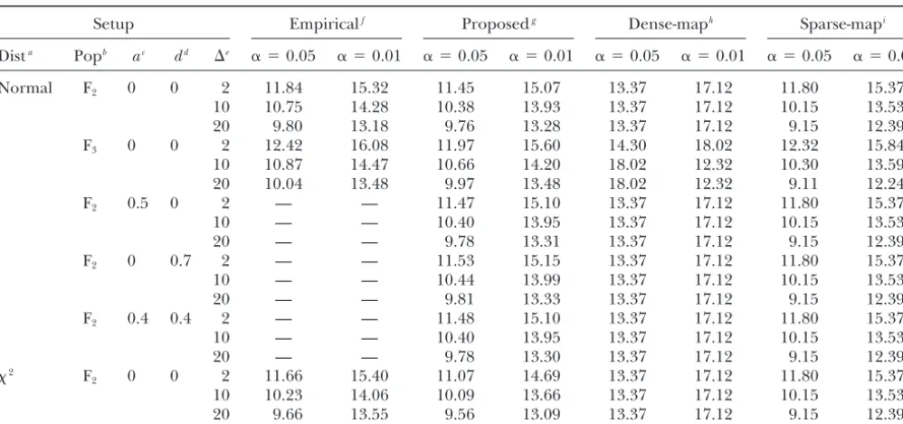
TABLE 1
Comparison of the proposed, theoretical, and empirical thresholds in an F2population and an advanced intercross F3population
Setup Empiricalf Proposedg Dense-maph Sparse-mapi
Dista Popb ac dd ⌬e ␣ ⫽0.05 ␣ ⫽0.01 ␣ ⫽0.05 ␣ ⫽0.01 ␣ ⫽0.05 ␣ ⫽0.01 ␣ ⫽0.05 ␣ ⫽0.01
Normal F2 0 0 2 11.84 15.32 11.45 15.07 13.37 17.12 11.80 15.37
10 10.75 14.28 10.38 13.93 13.37 17.12 10.15 13.53
20 9.80 13.18 9.76 13.28 13.37 17.12 9.15 12.39
F3 0 0 2 12.42 16.08 11.97 15.60 14.30 18.02 12.32 15.84
10 10.87 14.47 10.66 14.20 18.02 12.32 10.30 13.59
20 10.04 13.48 9.97 13.48 18.02 12.32 9.11 12.24
F2 0.5 0 2 — — 11.47 15.10 13.37 17.12 11.80 15.37
10 — — 10.40 13.95 13.37 17.12 10.15 13.53
20 — — 9.78 13.31 13.37 17.12 9.15 12.39
F2 0 0.7 2 — — 11.53 15.15 13.37 17.12 11.80 15.37
10 — — 10.44 13.99 13.37 17.12 10.15 13.53
20 — — 9.81 13.33 13.37 17.12 9.15 12.39
F2 0.4 0.4 2 — — 11.48 15.10 13.37 17.12 11.80 15.37
10 — — 10.40 13.95 13.37 17.12 10.15 13.53
20 — — 9.78 13.30 13.37 17.12 9.15 12.39
2 F
2 0 0 2 11.66 15.40 11.07 14.69 13.37 17.12 11.80 15.37
10 10.23 14.06 10.09 13.66 13.37 17.12 10.15 13.53
20 9.66 13.55 9.56 13.09 13.37 17.12 9.15 12.39
aError distribution. bMapping population (F
2or F3).
cAdditive effect. dDominant effect.
eMarker distance (in centimorgans).
fPercentiles of the test statistic based on the 10,000 simulated data sets under H
0.
gAverage of thresholds from 10,000 simulated data sets. hTheoretical thresholds based on the dense-map assumption. iTheoretical thresholds based on the sparse-map assumption.
since it is equivalent to the score test statistic in large limits ofn⫺12l(, ; d)/ andn⫺12l(, ;d)/2
asngoes to infinity [CoxandHinkley1974, Sect. 9.3 samples.
For the interval mapping of the F2 population, we (iii)]. Since Ui(d) involves only the information from theith subject, theUi(d) (i⫽1, . . . ,n) are independent write ⫽(a,b,,2) and we are interested in testing
the null hypothesis H0:⬅(a,b)⫽0 in the presence zero-mean random variables for any given d. Thus, it
follows from the multivariate central limit theorem that of the nuisance parameter⬅ (,2). In the sequel,
the general notation ofwill be used, wherepertains the process n⫺1/2U(d) is asymptotically a zero-mean
to the parameter of primary interest andto the nui- Gaussian process, where the covariance between n⫺1/2
sance parameter, so that general QTL models other U(d1) andn⫺1/2U(d2) at any two given positionsd1andd2
than the specific F2model are encompassed. is⌶(d1,d2), the limit ofn⫺1兺iUi(d1)UTi(d2). The
replace-LetU,i(;d)⫽li(,;d)/andU,i(;d)⫽li(, ment of the unknown parameters in (3) by their sample ;d)/. These are the contributions of theith subject estimators yields
to the score functions forand. Further, letU(d)⫽
Uˆi(d)⫽U,i(0,˜;d)⫺{2l(0,˜;d)/} {2l(0,˜;d)/2}⫺1
兺iU,i(0,˜;d), where˜ is the restricted MLE ofunder
H0: ⫽0,i.e., the solution of the equation兺iU,i(0,; ⫻U
,i(0,˜;d). (4)
d) ⫽ 0. Note that U(d) is the score function for 
evaluated at ⫽ 0 and ⫽ ˜. It follows from Taylor The restricted MLE ˜ in (4) may be replaced by the series expansions and the law of large numbers that unrestricted MLEˆ. By the law of large numbers and the
n⫺1/2U(d) has the same asymptotic distribution as consistency of the maximum-likelihood estimators,⌶(d 1,
n⫺1/2兺n
i⫽1Ui(d), where d2) can be consistently estimated by ⌶ˆ (d1, d2) ⫽
n⫺1兺n
i⫽1Uˆi(d1)UˆTi(d2).
Ui(d)⫽U,i(0,;d) The score test statistic for H
0: ⫽0 against H1:⬆0
at locationdtakes the form ⫺兺(0, ;d)兺⫺1
(0,;d)U,i(0, ;d), (3)
where Uˆ(d)⫽ 兺iUˆi(d) and Vˆ(d)⫽ n⌶ˆ (d,d) [Coxand that we are searching for multiple QTL in a backcross population. Given the genotypes of K QTL, the normal
Hinkley1974, Sect. 9.3 (iii)]. It can be shown thatW(d)
regression model takes the form is asymptotically equivalent to LRT(d) [CoxandHinkley
1974, Sect. 9.3 (iii)]. To assess the genome-wide statistical
y⫽ ⫹
兺
1ⱕkⱕK
xk␥k⫹
兺
1ⱕj⬆kⱕK
xjxk␥j k⫹e, (6)
significance, we need to evaluate the distribution of maxdW(d). In general, this is not analytically tractable. We
propose a resampling method similar to that ofLinet al. where xk is the QTL genotype indicator variable, which (1993) to approximate the distribution of maxdW(d). The takes the value⫺1 or 1 when thekth QTL is heterozygote idea of simulating thresholds using a score test statistic is or homozygote, respectively,is the grand mean,␥kis the mentioned inRebaiet al.(1994). main effect of thekth QTL,␥j kis the interaction between
Define the jth andkth QTL, ande is a zero-mean normal error
with variance2.
As in the case of the single-QTL analysis, the QTL
geno-U*(d)⫽
兺
n
i⫽1
Uˆi(d)Gi,
types are generally unobservable but the conditional proba-bilities of the QTL can be calculated given flanking markers. whereGi(i⫽1, . . . ,n) are independent standard normal
This results in the following mixture-model likelihood for random variables. Let
Kputative QTL locid1, . . . ,dK,
W*(d)⫽U*T(
d)Vˆ⫺1(d)U*(d). (5)
l(;d1, . . . ,dK)⫽
兺
ni⫽1
li(;d1, . . . ,dK), (7) In (5), we regard theUˆi(d) inU*(d) andVˆas fixed and
theGiinU*(d) as random. Conditional on the observable wherel
i(;d1, . . . ,dK)⫽ data, U*(d) is normal with mean 0 at each location d
and the covariance betweenn⫺1/2U*(d
1) andn⫺1/2U*(d2) log
冤
兺
a1,...,aK僆{⫺1,1}
i(a1, . . . ,aK;d1, . . . ,dK)φ equals⌶ˆ (d1,d2), which converges to⌶(d1,d2). It follows
that the conditional distribution ofn⫺1/2U*(d) given the
⫻
冦
yi⫺ ⫺兺1ⱕkⱕK ak␥k⫺兺1ⱕj⬆kⱕKakaj␥j k
冧冥
observed data converges to the same limiting distribution ofn⫺1/2Uˆ(d). Consequently, the distribution ofW(d) can
be approximated by that of W*(d). Our resampling andi(a1, . . . ,aK;d1, . . . ,dK)⫽ Pr(x1⫽ a1, . . . ,xK⫽ method is essentially a parametric bootstrap. aK|subjecti’s marker genotypes), which is the conditional We have shown that, under the null hypothesis, the probability of the joint genotypes of K QTL given the test statistics are functions of certain zero-mean Gaussian marker genotypes of theith subject. Let ⫽(,), where processes over the genome positions and the realizations  ⫽ (␥1, . . . ,␥K,␥12, . . . ,␥K⫺1,K) and ⫽ (,2). We from the Gaussian processes can be generated by Monte test the null hypothesis H0: ⫽0 against the alternative
Carlo simulations. In practice, the resampling procedure hypothesis H1:⬆0. Note that for MIM, the profile
likeli-is as follows: hood is calculated in K-dimensional space (d1, . . . ,dK).
Once the likelihood is obtained, the resampling procedure 1. SampleGi,i⫽1, 2, . . . ,n, fromN(0, 1). above can be applied to the resulting score test statistic 2. Calculate U*(d) ⫽ 兺n
i⫽1Uˆi(d)Gi, W*(d) ⫽ U*T(d) withd⫽(d
1, . . . ,dK). Vˆ⫺1(d)U*(d) andS*⫽max
dW*(d). For CIM, the model is essentially the same as MIM except
3. Repeat steps 1 and 2 a large number of times, say R that, for a given putative QTL position d, (x
1, . . . xK⫺1)
times. corresponding to the selected marker genotypes are known
4. For a given genome-wide type I error rate␣, calculate and onlyx
K corresponding to the putative QTL genotype the 100(1⫺ ␣)th percentile of theRvalues of theS*. is unobservable. Also, in CIM the interaction terms are If the observed value of the LRT exceeds this threshold, generally ignored. Thus for CIM, our mixture model will
then reject the null hypothesis. have likelihood (1) but l
i(; d) ⫽ log[兺aK僆{⫺1,1}i(aK;d)
φ((yi⫺ ⫺兺1ⱕkⱕK⫺1xk␥k⫹aK␥K)/)] and i(aK; d) ⫽ The above calculations are based on the score function
Pr(xK ⫽ aK|subjecti’s marker genotypes), the conditional and the observed information matrix from the original data.
probability of the genotypes of the putative QTL given the These quantities are evaluated once and used repeatedly in
marker genotypes of theith subject. In this situation, ⫽ step 2. Since it does not involve refitting the model in each
␥Kand ⫽(,␥1, . . . ,␥K⫺1,2).
iteration, the proposed method is computationally much more efficient than the permutation method. This is impor-tant with complex breeding designs and sophisticated QTL
SIMULATION STUDIES models (e.g., CIM and MIM), where the likelihood
calcula-tions are time consuming. Simulations were conducted to study the behavior of
Extensions to MIM/CIM:In this section, we show how the proposed method in an F2population. One
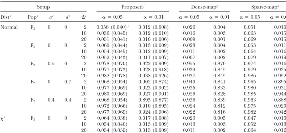
TABLE 2
Empirical type I error and power of the proposed and theoretical methods in an F2population and an advanced
intercross F3population
Setup Proposedf Dense-mapg Sparse-maph
Dista Popb ac dd ⌬e ␣ ⫽0.05 ␣ ⫽0.01 ␣ ⫽0.05 ␣ ⫽0.01 ␣ ⫽0.05 ␣ ⫽0.01
Normal F2 0 0 2 0.058 (0.040)i 0.012 (0.008) 0.026 0.004 0.051 0.010
10 0.056 (0.045) 0.012 (0.010) 0.016 0.003 0.063 0.015
20 0.051 (0.041) 0.010 (0.006) 0.009 0.001 0.069 0.015
F3 0 0 2 0.060 (0.044) 0.013 (0.009) 0.023 0.004 0.053 0.011
10 0.054 (0.045) 0.012 (0.009) 0.011 0.002 0.064 0.016
20 0.052 (0.043) 0.011 (0.007) 0.007 0.002 0.079 0.019
F2 0.5 0 2 0.978 (0.970) 0.922 (0.909) 0.955 0.870 0.974 0.916
10 0.977 (0.973) 0.928 (0.918) 0.939 0.845 0.979 0.935
20 0.982 (0.978) 0.938 (0.926) 0.937 0.845 0.986 0.952
F2 0 0.7 2 0.968 (0.954) 0.902 (0.874) 0.940 0.841 0.965 0.895
10 0.977 (0.969) 0.923 (0.902) 0.935 0.833 0.980 0.931
20 0.980 (0.969) 0.927 (0.901) 0.926 0.828 0.985 0.944
F2 0.4 0.4 2 0.968 (0.954) 0.895 (0.877) 0.936 0.839 0.963 0.888
10 0.972 (0.966) 0.910 (0.895) 0.924 0.812 0.975 0.920
20 0.977 (0.969) 0.924 (0.906) 0.922 0.816 0.982 0.942
2 F
2 0 0 2 0.064 (0.038) 0.017 (0.008) 0.023 0.005 0.047 0.010
10 0.054 (0.040) 0.013 (0.009) 0.013 0.003 0.052 0.013
20 0.054 (0.039) 0.015 (0.009) 0.011 0.002 0.064 0.016
aError distribution. bMapping population (F
2or F3).
cAdditive effect. dDominant effect.
eMarker distance (in centimorgans).
fType I error/power based on the proposed thresholds. gType I error/power based on the dense-map thresholds. hType I error/power based on the sparse-map thresholds.
iThe values in parentheses are type I error/power based onPiepho’s (2001) quick method.
markers were evenly spaced with a marker distance of tests have proper type I error and power. The theoretical thresholds based on the dense-map assumption are too 2, 10, or 20 cM. The null and alternative models were
simulated to investigate the type I error and power. conservative while those based on the sparse-map ap-proximation tend to be too liberal, especially for sparse Under the null hypothesis, the trait was randomly
sam-pled from the standard normal distribution. Under the maps. The results based on the method of Piepho
(2001) are also included in Table 2. As mentioned be-alternative, a QTL was simulated at 40 cM with different
additive and dominant effects. We set the sample size fore, Piepho’s method is generally conservative when the marker density is high. In contrast, the proposed to 200. We simulated 10,000 data sets for each
combina-tion of the marker distance and QTL effects. For each method is somewhat on the liberal side in small samples with dense maps. We may combine the proposed simulated data set, we setR⫽ 10,000 and␣ ⫽0.05 or
␣ ⫽ 0.01. The step width of the QTL scan is set to method with Piepho’s method when the marker density is relatively high.
1 cM for all simulations. To compare the resampling
method with the theoretical method, we also calculated To further assess the proposed method, we simulated a backcross population in searching for multiple QTL. the thresholds on the basis of the dense-map and
sparse-map approximations ofDupuis andSiegmund (1999) Again, one chromosome with a total length of 100 cM was simulated. Markers are evenly distributed with a as well as the corresponding type I error and power.
The results are summarized in Tables 1 and 2. To dem- distance of 2, 10, or 20 cM. The sample size is 300. A single QTL is located at 20 cM.
onstrate the generality of the proposed method,
simula-tions were also performed on an advanced intercross F3 When mapping multiple QTL, the analysis is done
either sequentially so that we search for the next most (see Tables 1 and 2).
The thresholds based on the proposed method match significant QTL after accounting for the effects of the identified QTL or jointly so that we search all QTL the empirical thresholds reasonably well, and the
thresh-olds are similar when the data are generated from the simultaneously. In the former, we search for a new gene conditional on previously identified genes.
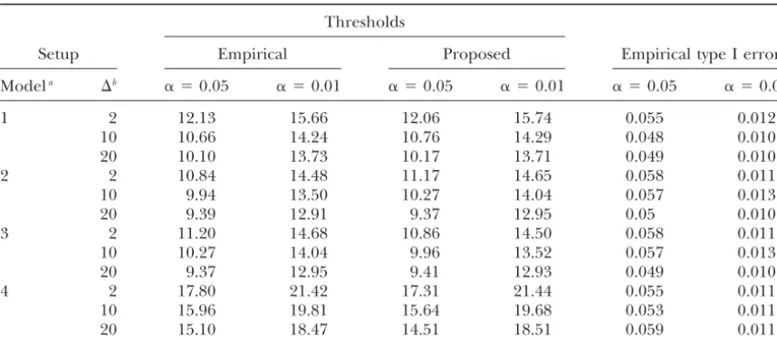
TABLE 3
Simulation results on the proposed thresholds and the corresponding empirical type I error in a backcross population
Thresholds
Setup Empirical Proposed Empirical type I error
Modela ⌬b ␣ ⫽0.05 ␣ ⫽0.01 ␣ ⫽0.05 ␣ ⫽0.01 ␣ ⫽0.05 ␣ ⫽0.01
1 2 12.13 15.66 12.06 15.74 0.055 0.012
10 10.66 14.24 10.76 14.29 0.048 0.010
20 10.10 13.73 10.17 13.71 0.049 0.010
2 2 10.84 14.48 11.17 14.65 0.058 0.011
10 9.94 13.50 10.27 14.04 0.057 0.013
20 9.39 12.91 9.37 12.95 0.05 0.010
3 2 11.20 14.68 10.86 14.50 0.058 0.011
10 10.27 14.04 9.96 13.52 0.057 0.013
20 9.37 12.95 9.41 12.93 0.049 0.010
4 2 17.80 21.42 17.31 21.44 0.055 0.011
10 15.96 19.81 15.64 19.68 0.053 0.011
20 15.10 18.47 14.51 18.51 0.059 0.011
aModels 1–3 are sequential tests, where search for the second QTL is conditional on the identified first
QTL. Under both models 1 and 2, we search the second QTL on the same chromosome of the first QTL. However, in model 1, the locus of the first QTL is fixed at its true location while in model 2, the first QTL locus is treated as unknown and the marker closest to the locus with the maximum LOD is chosen as the estimated position of the first QTL. Model 3 is similar to model 1, except that we search the second QTL on a different chromosome of the first QTL. Model 4 fits the MIM model with two QTL fitted simultaneously.
bMarker distance (in centimorgans).
For the sequential analysis, either we assumed that The results of the sequential analysis under␥1⫽1 and
␥2⫽ ␥12⫽0 are summarized in Table 3. The proposed
the position of the first QTL is known (at 20 cM), and
given this QTL, we searched for the second QTL, or we thresholds are again close to the empirical levels and have proper control of the type I error regardless of assumed that the position of the first QTL is unknown
and the marker closest to the locus with the maximum whether the first QTL locus is fixed at its true position or selected with the results of the single-QTL interval LOD is selected as the locus for the first QTL. Regardless
of the method used to choose the position of the first mapping. Additional simulations (not shown) demon-strate that the resampling thresholds for data generated QTL, we tested the null hypothesis H0: ␥2 ⫽ ␥12 ⫽ 0
under model (6) against the alternative hypothesis H1: under alternatives with two QTL are similar to those of
Table 3, so that the resampling method yields adequate ␥2 ⬆ 0 or/and␥12⬆ 0 across the whole chromosome.
We treatedx1as fixed and calculated the profile likeli- power.
As shown in Table 3, when we search for the second hood at all possible loci for the second QTL.
If the putative QTL locus is very close to the primary gene on a different chromosome from the chromosome where the first gene resides, the thresholds are slightly QTL, the collinearity between x1 and x2 will be very
strong, which may result in relatively high LOD scores lower than when we search for the second gene on the same chromosome as that of the first gene. This suggests in a region very close to the primary QTL. To investigate
this, we simulated another chromosome that is also 100 that to retain the power to detect genes not linked to the primary gene, we may partition the whole genome cM long and searched the second QTL only on the
second chromosome. into two groups, one linked with the primary QTL and
one unlinked with the primary QTL. The LOD scores The above two cases are examples of the CIM analysis
in which only one marker, instead of several, is used as within each group can then be compared to the corre-sponding threshold. We can also exclude a small region, the covariate in the analysis. To show the strength of the
proposed method in multiple-QTL mapping (MIM), say 10 cM to the left and to the right of the primary QTL to break down the high collinearity between x1
where the computational demand for permutation tests
is very high, we also simulated two 100-cM chromosomes andx2, as in the case with CIM.
For MIM, we fit model (6), where neither x1 nor x2
and fit a two-QTL model to investigate how the type I
errors are controlled under the global null hypothesis is observed and the profile likelihood is calculated for all possible locus combinations of the first and second of no QTL present. For simplicity, we restricted our
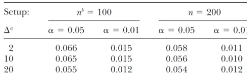
TABLE 4 procedure (the recorded CPU times of the resampling and permutation procedures running on an IBM Blade-Empirical type I error of the proposed method in an F2
Center HS20 machine are 13 and 6000 sec, respectively). population with missing genotype data
The derived 95% thresholds are 10.08 and 9.96 from the proposed and permutation methods, respectively.
nb⫽100 n⫽200
Setup:
The corresponding 99% thresholds are 13.49 and 13.46.
⌬a ␣ ⫽0.05 ␣ ⫽0.01 ␣ ⫽0.05 ␣ ⫽0.01
The two procedures result in very similar thresholds, 2 0.066 0.015 0.058 0.011 but the proposed method takes far less computing time.
10 0.065 0.015 0.056 0.010 The LOD score profile of the original data and the
20 0.055 0.012 0.054 0.012 estimated 95% threshold are plotted in Figure 1. The genetic signals on all three chromosomes are very The average missing genotype rate at each marker is 10%.
strong. As suggested inZenget al.(2000), as many as 19 aMarker distance (in centimorgans).
bSample size.
different QTL controlling this morphometric descriptor may exist. For these complicated real data, where some of our assumptions, such as normality, are likely to fail, the single-QTL analysis andK is the total number of the thresholds from permutation and our proposed pro-QTL fitted in MIM, which is a dramatic increase relative cedures agree very well. Since the permutation proce-to CIM. We performed 1000 simulations for MIM. As dure is known to be robust to those violations, this shown in Table 3, the proposed method works reason- real example further demonstrates the usefulness of the ably well for MIM mapping and the type I errors are proposed method. To further compare the permutation
well controlled. and proposed method, we provided a QQ-plot (Figure
To investigate the robustness of the proposed 2) of the permutation- and the resample-based null dis-method, we also simulated situations with smaller sam- tribution estimates of the maximum profile likelihood-ple sizes, missing marker genotypes, and2
1-distributed ratio test statistic. The two estimated distributions match
traits. The results for2
1traits are presented in the bot- rather well up to the 99.5th percentile. The discrepancy
tom three rows of Tables 1 and 2. The type I error is in the tails of the distributions may be due, in part, to only slightly inflated for␣ ⫽ 0.05. As shown in Table the limited number of resamplings and permutations. 4, the performance of the proposed method is also fairly To improve the accuracy of the estimates of the null insensitive to missing genotype data and small sample distribution in the tail, a larger number of resamplings sizes. With sample size 100 and 10% missing marker and permutations are necessary. For comparison, we genotypes, the type I error is still close to the nominal also calculated the 95 and 99% thresholds byPiepho’s
level. (2001) method, which are 11.23 and 14.44, respectively.
Those thresholds are slightly larger than both the per-mutation-based and our resampling-based thresholds. APPLICATION TO A DROSOPHILA BACKCROSS
We use a Drosophila data set (Zenget al. 2000) to
DISCUSSION compare the permutation procedure with the proposed
method. Two closely related allopatric species,Drosoph- In this article, we propose a new empirical method to calculate the threshold for QTL mapping. The
ila simulansandD. mauritiana, differ dramatically in the
size and shape of the posterior lobe of the male genital method is far more efficient than the popular permuta-tion procedure since the proposed method needs to arch. To investigate the genetic architecture of the
mor-phometric difference between the two species, female maximize the likelihood of the observed data only once with no need to maximize the likelihood in each
resam-D. simulans were crossed to males of D. mauritiana to
generate an F1 population. The F1 females were back- pling iteration any more. For standard interval mapping
with simple crosses, the resampling method is several crossed to parental lineD. simulansand 299 backcross
males were produced. A morphometric descriptor, re- hundred times faster than the permutation procedure. Furthermore, the proposed method is applicable to ferred to as PC1 by Zenget al.(2000), is the average
over both sides of the first principal components of the more complicated designs and models that cannot be handled by the permutation procedure. For example, Fourier coefficients of the posterior lobe and is used to
quantify both the size and shape variation. There are for MIM where the model selection is involved, the bootstrap resampling method ofZeng et al.(1999) is 42 markers unevenly distributed on the X chromosome
and on chromosomes 2 and 3. Interval mapping was applicable to the linear regression model but may not be applicable to nonlinear models, such as logistic re-performed across all three chromosomes. The step size
of the QTL scan was 1 cM. Threshold calculations were gression and Poisson regression. The proposed method also avoids the derivation of parameters in the Ornstein-based on 10,000 permutations and resamples. Our
re-corded running time showed that the proposed method Uhlenbeck diffusion approximations, which can be a difficult task when the model is complicated.
Figure1.—The LOD profile for chro-mosomes X, 2, and 3 from interval map-ping. The solid horizontal line is the 95% resampling threshold, which is al-most identical to the 95% permutation threshold (the dashed horizontal line).
The computational advantage of the proposed critical, even with the current trend in computing power.
method over the permutation procedure depends on
how complex the original model is. The more compli- The simulations indicated that for simple interval mapping with F2 or backcross, either the restricted or
cated the model is, the more there is to be gained from
the proposed method. In the Drosophila analysis, where unrestricted estimator of can be used and the two estimators tend to give very similar thresholds. However, a simple interval-mapping model was fitted on three
chromosomes, there was a decrease in computing time for the two-gene model, we found that the unrestricted estimator of works slightly better than the restricted in the order of 102. If more complicated models, such
as multiple-QTL mapping or CIM, are used, where max- one. For this reason, we suggest the use of the un-restricted estimator of the nuisance parameters in evalu-imization via the EM algorithm is more time consuming,
the proposed method may be thousands of times faster ating the thresholds, and the simulation results pre-sented in this article are based on an unrestricted than the permutation procedure. With the recent efforts
to map the gene expression levels of thousands of genes estimator of.
The simulations also showed that the proposed via microarrays (Lan et al. 2003), an efficient way to
Figure 2.—The QQ-plot of the esti-mated null distributions from the pro-posed method and the empirical permu-tation method in the Drosophila data analysis. The two vertical dashed lines are the 95 and 99% thresholds from the proposed method. The solid diagonal line represents the situation when the two estimated distributions were identi-cal. The actual estimated distributions are represented by the points along this diagonal line.
data. Though the normal model is used to fit the non- generally conservative when the marker density is high, the proposed method is somewhat on the liberal side normal chi-square data, the empirical type I error from
the proposed method is reasonably controlled at the in small samples with dense maps. We may consider combining the proposed method with Piepho’s method targeted level. However, it is unclear how this method
will work for data with segregation distortion, which is when the marker density is relatively high. a complex phenomenon. Due to different mechanisms
of segregation distortion, it is difficult to predict the
LITERATURE CITED performance of the method. If the existence of
segrega-tion distorsegrega-tion is suspected, a simple solusegrega-tion is to re- Basten, C. J., B. S. WeirandZ-B. Zeng, 1997 QTL Cartographer: A Reference Manual and Tutorial for QTL Mapping.Department of move those markers that are in segregation distortion
Statistics, North Carolina State University, Raleigh, NC. from the analysis. Including markers in segregation dis- Broman, K. W., 2001 Review of statistical methods for QTL mapping tortion in the analysis will result in a distorted map in experimental crosses. Lab Anim.30:44–52.
Churchill, G. A., and R. W. Doerge, 1994 Empirical threshold estimate and may give biased mapping results,
regard-values for quantitative trait mapping. Genetics138:963–971. less of the method used to compute the thresholds. Cox, D., andC. Hinkley, 1974 Theoretical Statistics.Chapman &
Reference Manual for MAPMAKER/QTL. Whitehead Institute, Cam-is present only under the alternative. Biometrika64:247–254.
bridge, MA.
Davies, R. B., 1987 Hypothesis testing when a nuisance parameter
Lynch, M., andB. Walsh, 1998 Genetics and Analysis of Quantitative
is present only under the alternative. Biometrika74:33–43.
Traits.Sinauer Asociates, Sunderland, MA.
Dempster, A. P., N. M. LairdandD. B. Rubin, 1977 Maximum
Manly, K. F., andJ. M. Olson, 1999 Overview of QTL mapping likelihood from incomplete data via the EM algorithm. J. R. Stat.
software and introduction to Map Manager QT. Mamm. Genome Soc.39:1–38.
10:327–334.
Doerge, R. W., 2001 Mapping and analysis of quantitative trait loci
Piepho, H. P., 2001 A quick method for computing approximate in experimental populations. Nat. Rev. Genet.3:43–52.
thresholds for quantitative trait loci detection. Genetics157:425–
Dupuis, J., andD. Siegmund, 1999 Statistical methods for mapping
432. quantitative trait loci from a dense set of markers. Genetics151:
Rebai, A., B. GoffinetandB. Mangin, 1994 Approximate thresh-373–386.
olds of interval mapping tests for QTL detection. Genetics138:
Jansen, R. C., andP. Stam, 1994 High resolution of quantitative
235–240. traits into multiple quantitative trait in line crosses using flanking
Rebai, A., B. GoffinetandB. Mangin, 1995 Comparing power of markers. Genetics136:1447–1455.
different methods for QTL detection. Biometrics51:87–99.
Kao, C. H., andZ-B. Zeng, 1997 General formulas for obtaining
Zeng, Z-B., 1993 Theoretical basis of separation of multiple linked the maximum likelihood estimates and the asymptotic
variance-gene effects on mapping quantitative trait loci. Proc. Natl. Acad. covariance matrix in QTL mapping when using the EM algorithm.
Sci. USA90:10972–10976. Biometrics53:653–665.
Zeng, Z-B., 1994 Precision mapping of quantitative traits loci.
Genet-Kao, C. H., Z-B.Zengand R. D.Teasdale, 1999 Multiple interval
ics136:1457–1468. mapping for quantitative trait loci. Genetics152:1203–1216.
Zeng, Z-B., C. H. KaoandC. J. Basten, 1999 Estimating the genetic
Lan, H., J. P. Stoehr, S. T. Nadler, K. L. Schueler, B. S. Yandell architecture of quantitative traits. Genet. Res.74:279–289.
et al., 2003 Dimension reduction for mapping mRNA abun- Zeng, Z-B., L. Liu, L. F. Stam, C. H. Kao, J. M. Merceret al., 2000 dance as quantitative traits. Genetics164:1607–1614. Genetic architecture of a morphological shape difference
be-Lander, E. S., andD. Botstein, 1989 Mapping Mendelian factors tween two Drosophila species. Genetics154:299–310.
underlying quantitative traits using RFLP linkage maps. Genetics Zou, F., B. S. YandellandJ. P. Fine, 2001 Statistical issues in the
121:185–199. analysis of quantitative traits in combined crosses. Genetics158:
Lin, D. Y., L. J. WeiandZ. Ying, 1993 Checking the Cox model 1339–1346. with cumulative sums of martingale-based residuals. Biometrika