A Monte Carlo EM Algorithm for Generalized Linear Mixed Models with Flexible Random Effects Distribution

(1)

Abstract

CHEN, JUNLIANG. A Monte Carlo EM algorithm for generalized linear mixed models

with flexible random effects distribution. (Under the direction of Daowen Zhang and Marie

Davidian)

A popular way to model correlated binary, count, or other data arising in clinical trials

and epidemiological studies of cancer and other diseases is by using generalized linear mixed

models (GLMMs), which acknowledge correlation through incorporation of random effects.

A standard model assumption is that the random effects follow a parametric family such

as the normal distribution. However, this may be unrealistic or too restrictive to represent

the data, raising concern over the validity of inferences both on fixed and random effects if

it is violated.

Here we use the seminonparametric (SNP) approach (Davidian and Gallant 1992, 1993)

to model the random effects, which relaxes the normality assumption and just requires that

the distribution of random effects belong to a class of “smooth” densities given by Gallant

and Nychka (1987). This representation allows the density of random effects to be very

flexible, including densities that are skewed, multi–modal, fat– or thin–tailed relative to

(2)

representation to avoid numerical instability in estimating the polynomial coefficients.

Because an efficient algorithm to sample from a SNP density is available, we propose

a Monte Carlo expectation maximization (MCEM) algorithm using a rejection sampling

scheme (Booth and Hobert, 1999) to estimate the fixed parameters of the linear predictor,

variance components and the SNP density. A strategy of choosing the degree of flexibility

required for the SNP density is also proposed. We illustrate the methods by application

to two data sets from the Framingham and Six Cities Studies, and present simulations

(3)

A MONTE CARLO EM ALGORITHM FOR

GENERALIZED LINEAR MIXED MODELS WITH

FLEXIBLE RANDOM EFFECTS DISTRIBUTION

by

JUNLIANG CHEN

A dissertation submitted to the Graduate Faculty of North Carolina State University

in partial fulfillment of the requirements for the Degree of

Doctor of Philosophy

STATISTICS

Raleigh

2001

approved by:

Dennis D. Boos Sujit Ghosh

Daowen Zhang Marie Davidian

(4)

(5)

Biography

CHEN, JUNLIANG was born on September 22, 1972 in Huangmei, Hubei province, P.R.China.

He entered the Department of Mathematics at Nankai University in Tianjin, P.R.China in

1991, and received a B.S. degree in Mathematical Statistics there in 1995. After two years

graduate study, he decided to join the graduate program in Statistics at North Carolina

State University in August 1997. He earned his M.S. in Statistics in 1999 and continued

(6)

Acknowledgments

First of all, I would like to express my deepest appreciation to my advisors, Dr. Daowen

Zhang and Dr. Marie Davidian, for their guidance, encouragement and patience throughout

the development of my doctoral research and the preparation of my thesis. I would also

like to thank the rest of my advisory committee for their review of this work and many

valuable suggestions.

I gratefully acknowledge the Faculty in Statistics at North Carolina State University

for their high quality instruction and guidance. I thank my friends, including my fellow

graduate students and my fellow statisticians at SAS, for their assistance and friendship.

Finally, I thank all of my family, including my in–laws, for their support through this

process. I especially want to thank my wife Lihua for her love, encouragement, support

and patience, and my daughter Jessica who gave me so much pleasure during the course of

(7)

List of Tables

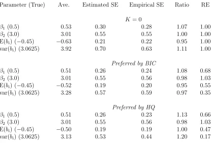
5.1 Simulation results for 100 binary data sets: mixture scenario . . . 71

5.2 Simulation results for 100 binary data sets: normal scenario . . . 72

5.3 Simulation results for 100 continuous data sets: mixture scenario . . . 78

5.4 Simulation results for 100 continuous data sets: normal scenario . . . 79

6.1 Results for the Six Cities study . . . 85

(10)

List of Figures

2.1 SNP densities with different estimates of coefficients in polynomial . . . 19 2.2 SNP density function with ψ = (0.58,1.56), µ=−0.11 andσ2 _{= 1}_._{58. . . .} ₂₆ 2.3 SNP density function with ψ = (−0.66,−1.21), µ=−0.01 andσ2 _{= 1}_._{61. .} ₂₇ 2.4 SNP density function with ψ = (0.30,1.57), µ=−0.2 and σ2 = 2.33. . . 28 2.5 SNP density function with ψ = (−0.36,−1.20), µ=−0.12 andσ2 _{= 2}_._{68. .} ₂₉ 2.6 Histogram of a random sample generated from a SNP density . . . 34

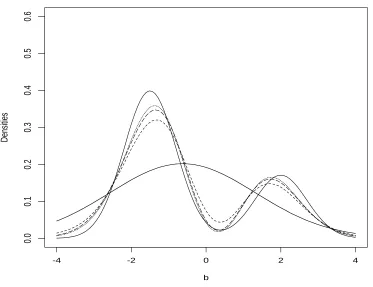
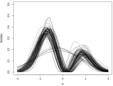
5.1 Averages of estimated densities for 100 binary data sets: mixture scenario. 73 5.2 100 estimated densities chosen by HQ for binary data sets: mixture scenario. 74 5.3 Averages of estimated densities for 100 continuous data sets: mixture scenario. 80 5.4 100 estimated densities chosen by HQ for continuous data sets: mixture

scenario. . . 81 5.5 15 estimated densities where K >0 was chosen by AIC for continuous data

sets: normal scenario. . . 82

6.1 Estimated random effects densities for fits to the Six Cities data. . . 86 6.2 Longitudinal cholesterol levels for five randomly chosen subjects. . . 90 6.3 Histogram of individual least squares intercept estimates in the cholesterol

(11)

Chapter 1 Introduction

1.1 Background

1.1.1 Motivation

A popular way to model correlated binary, count, or other data is by using generalized linear

mixed models, which accommodate correlation through incorporation of random effects. A

standard assumption is that the random effects are normally distributed; however this may

be unrealistic to represent the variation in the data.

In this thesis, we consider generalized linear mixed models where the random effects

are assumed only to have a “smooth” density. To fit this more flexible model, we propose

a Monte Carlo expectation–maximization (EM) algorithm that is straightforward to

im-plement. We also propose a strategy to choose the degree of flexibility required. In the

(12)

1.1.2 Generalized Linear Mixed Models

Generalized linear models (Nelder and Wedderburn 1972; McCullagh and Nelder 1989)

have been shown to unify the approach to regression for a wide variety of discrete and

continuous data, such as binary, count, and other data. They retain the linearity through

the incorporation of link functions.

Suppose data y_i given x_i, i = 1, . . . , m, are independent and arise from an exponential dispersion family with the following probability density function (pdf) or probability mass

function (pmf),

f(y_i;θ_i, φ) = exp

½

y_iθ_i−d(θ_i)

a(φ) +c(yi;φ)

¾

, (1.1)

where φ is a dispersion parameter whose value may be known; d(·), a(·) and c(·;·) are known functions. A generalized linear model assumes that µ_i = E(y_i) =d0(θ_i), is related to the covariates x_i through a link functiong(·), and the linear predictor η_i is given by

η_i =xT_i β =g(µ_i),

(13)

has probability mass function

f(y_i;π_i) =π_iyi(1−π_i)1−yi _{= exp}

½

y_ilog

µ

π_i

1−π_i

¶

+ log(1−π_i)

¾

.

Therefore, θ_i = log{π_i/(1−π_i)}, µ_i =π_i, and the logit link function is the canonical link, since

η_i =g(µ_i) = log

µ

π_i

1−π_i

¶

=θ_i.

A list of canonical link functions for some common univariate distributions in the

exponen-tial family can be found in Section 2.2 of McCullagh and Nelder (1989).

One natural principle for fitting generalized linear models is maximum likelihood

es-timation. Some standard numerical evaluation techniques are available to maximize the

log–likelihood function, such as the Newton–Raphson and Fisher scoring methods. It turns

out that the Fisher scoring method for generalized linear models can be implemented by

iteratively reweighted least squares (McCullagh and Nelder, 1989).

We usually use generalized linear models to analyze a wide variety of responses that

are assumed to be independent. However, the response data collected in some biomedical

studies might be correlated. For example, in a longitudinal study, repeated measures for

one subject are collected over time and hence are correlated. In a genetic study, data

collected among members of the same family are correlated since the family members share

a similar genetic factor. Linear mixed models (Laird and Ware, 1982), where random

effects are used to model the correlation in data, have become a popular framework for

(14)

levels of variability: random variation among measurements within a given unit and random

variation among units. Under the assumptions of normality and independence for these two

levels of random variation, the normal theory estimation of variance components can be

developed. Two important methods, maximum likelihood (ML) and restricted maximum

likelihood (REML) estimation, are described by Davidian and Giltinan (1995) in Section

3.3.

The class of generalized linear mixed models, GLMMs, (Schall 1991; Zeger and Karim

1991), which subsumes certain linear mixed models, extends the strategy of incorporation of

random effects to the generalized linear models. It is a popular way to represent correlated

binary, count or other data arising in clinical trials and epidemiological studies of cancer

and other diseases.

Let y_ij denote the jth response for the ith individual, i = 1, . . . , m and j = 1, . . . , n_i. For each i, conditional on random effects b_i (q×1), the y_ij, j = 1, . . . , n_i are assumed to be independent and follow a generalized linear model (McCullagh and Nelder, 1989) with

density

f(y_ij|b_i;β, φ) = exp

½

y_ijθ_ij −d(θ_ij)

a(φ) +c(yij;φ)

¾

, (1.2)

where µ_ij = E(y_ij|b_i) = d0(θ_ij); φ is a dispersion parameter whose value may be known;

d(·),a(·) andc(·; ·) are known functions; and, for link functiong(·), the linear predictor

(15)

x_ij and s_ij for the fixed and random effects, respectively.

If we assume that the random effects b_i have a parametric density f(b_i;δ) which de-pends on parameters δ for each i, the specification of the generalized linear mixed model is completed, and the marginal likelihood for ζ can be written as

L(ζ;y) =

Z

f(y|b;β, φ)f(b;δ)db, (1.3)

where ζ is made up ofβ, φ and δ;

f(y|b;β, φ) =

m Y

i=1

f(y_i|b_i;β, φ),

f(y_i|b_i;β, φ) =

ni

Y

j=1

f(y_ij|b_i;β, φ), (1.4)

and

f(b;δ) =

m Y

i=1

f(b_i;δ);

(16)

1.1.3 EM Algorithm

The Expectation–Maximization (EM) algorithm was popularized by Dempster, Laird and

Rubin (1977). It is a clever way to compute complicated maximum likelihood estimation

from incomplete data such as missing, censored or truncated data. The name of EM

algorithm implies that it consists of an iterative computation of an expectation step followed

by a maximization step.

Let (x, y) be the “complete” data with the density function f(x, y;θ); x are missing data, y are observed data. The marginal likelihood function of θ given observed data y is given by

L(θ;y) = f(y;θ) =

Z

f(x, y;θ)dx. (1.5)

However, it is usually difficult to obtain a closed form for (1.5) for many applications. In

some cases, the EM algorithm can still obtain the MLE ofθmaximizingL(θ;y) numerically without having to do the integration in (1.5). Note that f(x, y;θ) =f(x|y;θ)f(y;θ). Thus we can write

logf(y;θ) = logf(x, y;θ)−logf(x|y;θ).

Now, suppose θ(r) _{is the value of} _θ _{at the} _r_{th iteration. Taking conditional expectations} given y for both sides, evaluated at θ(r) _yields

(17)

Let

Q(θ|θ(r)) = E_θ(r){logf(x, y;θ)|y},

and

H(θ|θ(r)) = E_θ(r){logf(x|y;θ)|y}.

The EM algorithm takes the form of an iterative procedure that, given therth iterateθ(r), we calculate Q(θ|θ(r)) in the expectation step and maximize Q(θ|θ(r)) with respect to θ in the maximization step to obtain θ(r+1). Each iteration will increase the log–likelihood. To show this, we consider the difference

logL(θ(r+1);y)−logL(θ(r);y)

= Q(θ(r+1)|θ(r))−Q(θ(r)|θ(r))− {H(θ(r+1)|θ(r))−H(θ(r)|θ(r))}.

Asθ(r+1) maximizesQ(θ|θ(r)) with respect toθ at the maximization step givenθ(r), it must be that

(18)

In addition, we have

H(θ(r+1)|θ(r))−H(θ(r)|θ(r))

= E_θ(r) ©

logf(x|y;θ(r+1))|yª−E_θ(r) ©

logf(x|y;θ(r))|yª

= Z ©logf(x|y;θ(r+1))ªf(x|y;θ(r))dx−Z ©logf(x|y;θ(r))ªf(x|y;θ(r))dx

=

Z ½

log f(x|y;θ (r+1)₎

f(x|y;θ(r)₎

¾

f(x|y;θ(r))dx.

Note that by Jensen’s inequality (Shorack, 2000, Sec. 3.4), since log(·) is a concave function,

we have

Z ½

log f(x|y;θ (r+1)₎

f(x|y;θ(r)₎

¾

f(x|y;θ(r))dx

≤ log

½Z

f(x|y;θ(r+1))

f(x|y;θ(r)₎ f(x|y;θ (r)_)d_x

¾

= log

½Z

f(x|y;θ(r+1))dx

¾

= 0.

Thus, putting everything together, we have shown that

logL(θ(r+1);y)−logL(θ(r);y)≥0.

Under some regularity conditions, Dempster, Laird and Rubin (1977) showed that the

(19)

calculate and maximize. This is the case for a large class of problems, in particular, if the

underlying “complete” data come from an exponential family. For example, the application

of EM algorithm for usual linear mixed model was described by Laird and Ware (1982) and

Davidian and Giltinan (1995, Sec. 3.4). However, it is not always the case that we can find

a closed form for Q(θ|θ(r)), particularly for generalized linear mixed models. The Monte Carlo EM (MCEM) algorithm was developed by using a Monte Carlo approximation in the

E–step when the required integration may not be carried out analytically. More details on

the MCEM algorithm are in Chapter 3.

1.2 Literature Review

In contrast to generalized linear models and general linear mixed models, the estimation of

fixed effects β, dispersion parameter φ, and parameters specifying the distribution of the random effects in generalized linear mixed models is more complicated since the random

effects enter the models nonlinearly. The marginal likelihood, which requires the integration

over the distribution of random effects as in (1.3), may not have a closed form even for

normal random effects. Consequently, much work has focused on approximate techniques

that try to avoid the difficulty of integration.

Schall (1991) used the first order expansion of the link function g(·) applied to the data at the conditional mean µ and obtained the working vector (McCullagh and Nelder, 1989). This allows the model to be reduced to a linear mixed model by using the working

(20)

flexible random effects and just requires one to specify the variance function of the random

effects. However, this approximation based on the first order expansion may be very poor,

especially for binary responses.

Breslow and Clayton (1993) applied penalized quasi–likelihood (PQL) and marginal

quasi–likelihood (MQL) methods for the generalized linear mixed models. The key

as-sumption of using PQL is that the random effects are assumed to arise from a multinormal

distribution. These authors used Laplace’s method for the normal integral approximation

(Barndorff–Nielsen and Cox, 1989) and derived the score equations for the mean parameters

by using several ad hoc adjustments and approximations. For marginal quasi–likelihood, they derived the marginal models by using the first order approximation to the hierarchical

model. These methods may not be accurate because of the approximations, even though

they are adequate to provide starting values for use with other, more exact procedures.

Breslow and Lin (1995) and Lin and Breslow (1996) investigated the bias of these kinds of

estimators and provided bias–correction methods.

Alternatively, fully Bayesian analysis implemented via Markov chain Monte Carlo

tech-niques and expectation maximization algorithms was proposed by several authors. An

attractive feature of these methods is that they allow assessment the uncertainty in the

estimated random effects and functions of model parameters.

Zeger and Karim (1991) proposed an algorithm based on the Bayesian framework by

using a Gibbs sampling approach (Gelfand and Smith, 1990) to get the sample points from

(21)

Some authors proposed Monte Carlo EM algorithms for generalized linear mixed

mod-els. Expectation maximization algorithms (Dempster, Laird and Rubin, 1977) are usually

used to avoid difficult integration in complicated problems, provided that the conditional

expectation at the E–step and maximization at the M–step are easy to calculate. However,

we may not have a closed form for the conditional expectation of the log–likelihood at the

E–step for the generalized linear mixed models. Consequently, Monte Carlo approximation

at the E–step leads to a Monte Carlo EM algorithm.

McCulloch (1997) proposed a Monte Carlo EM algorithm for generalized linear mixed

models by using Metropolis–Hastings algorithm (Tanner, 1993) to produce random draws

from the conditional distribution of random effects given the observed data. The advantage

of using Metropolis–Hastings algorithm is that the calculation of acceptance probability

only depends on the specification of the conditional distribution of y_i|b_i; namely, the form of (1.4).

Booth and Hobert (1999) proposed another Monte Carlo EM algorithm by using a

rejection sampling scheme to construct a Monte Carlo approximation at the E–step.

Com-pared to the MCEM algorithm (McCulloch, 1997), the random draws by using a rejection

sampling method are independent and identically distributed. This has the advantage that

one can assess the Monte Carlo error at each iteration by using standard central limit

theory combined with the first–order Taylor series. This suggests a rule for automatically

increasing the Monte Carlo sample size after iterations in which the change of the

parame-ter values is swamped by Monte Carlo error. This generally saves considerable computing

(22)

However, the implementation of these algorithms (Breslow and Clayton, 1993; Zeger and

Karim, 1991; McCulloch, 1997; and Booth and Hobert, 1999) requires the assumption that

the random effects have distribution belonging to some parametric family, almost always the

normal. This implies symmetry and unimodality of the random effects distribution. But,

this may be unrealistic or too restrictive to represent the real data. Moreover, prediction of

individual unit effects may be compromised because of the misspecification of the random

effects distribution, raising concern over the validity of inferences both on fixed and random

effects if it is violated. Allowing the random effects distribution to have more complex

features than the symmetric, unimodal normal density may provide insight into underlying

heterogeneity of the population of units and even suggest failure to include important

covariates in the model.

Accordingly, considerable interest has focused on approaches that allow the parametric

assumption to be relaxed in mixed models (Davidian and Gallant, 1993; Madger and Zeger,

1996; Verbeke and Lesaffre, 1996; Kleinman and Ibrahim, 1998; Aitken, 1999; Jiang, 1999;

Tao et al., 1999; Zhang and Davidian, 2001). Many of these approaches assume only that the random effects distribution has a “smooth” density and represent the density in

different ways. In particular, for a general nonlinear mixed model (NLMM), Davidian and

Gallant (1992, 1993) assumed that the random effects have a “seminonparametric” (SNP)

density in a “smooth” class given by Gallant and Nychka (1987), which includes normal

distribution as a special case. Numerical integration was used to compute the likelihood.

Zhang and Davidian (2001) proposed use of the “seminonparametric” (SNP) representation

(23)

likelihood to be expressed in a closed form, facilitating straightforward implementation.

They showed that this approach yields attractive performance in capturing features of the

true random effects distribution and has potential for substantial gains in efficiency over

normal–based methods.

In this dissertation, we apply this technique to the more general class of GLMMs.

Although it is no longer possible to write the likelihood in a closed form, the fact that an

efficient algorithm is available for sampling from a SNP density allows an extension of the

Monte Carlo EM algorithm of Booth and Hobert (1999) to the case of a “smooth” but

unspecified random effects density involving no much greater computational burden than

when a parametric family is specified. In Chapter 2, we introduce and present the form of

SNP density, describe an algorithm to generate a random sample from a SNP density by

using acceptance–rejection methods. More details about Monte Carlo EM algorithm can be

found in Chapter 3. The semiparametric GLMM and the strategy to choose the degree of

flexibility required for the SNP density are described in Chapter 4. We present simulations

demonstrating performance of the approach and illustrate the methods by application to

(24)

Chapter 2 Seminonparametric Density

2.1 Introduction

The term “seminonparametric” or SNP was used by Gallant and Nychka (1987), to suggest

that it lies halfway between fully parametric and completely nonparametric specifications.

Gallant and Nychka (1987) showed that the SNP method, which is based on a truncated

version of the infinite Hermite series expansion, may be used as a general–purpose

approx-imation to densities satisfying certain smoothness restrictions, including differentiability

conditions, such that they may not exhibit unusual behavior such as kinks, jumps, or

os-cillation. However, they may be skewed, multi–model, fat– or thin–tailed relative to the

normal distribution, and also contain the normal as a special case. A full mathematical

description of “smooth” densities was given by Gallant and Nychka (1987). Thus, the

densities under certain smoothness restriction allow for the possibility of a wide range of

(25)

situations.

We give a detailed description of SNP parameterization in Section 2.3. An algorithm

to generate a random sample from a SNP density is described in Section 2.4.

2.2 SNP Models

Following Davidian and Gallant (1993) and Zhang and Davidian (2001), we propose to

represent the SNP density in the semiparametric generalized linear mixed model (SGLMM)

by the truncated version of the infinite Hermite series expansion, which we now describe.

More details in SGLMM can be found in Chapter 4.

Suppose Z is aq–variate random vector with density proportional to a truncated Her-mite expansion so that Z has density

h_K(z)∝P_K2(z)ϕ_q(z) (2.1)

for some fixed value of K, where P_K(z) is a multivariate polynomial of orderK, andϕ_q(·) is the density function of the standard q–variate normal distribution with mean 0 and variance–covariance matrix I_q. Thus, for example, with z = (z₁, z₂)T_, _q_{= 2, and} _K _{= 2,}

(26)

The proportionality constant is given by

1

R

P2

K(s)ϕq(s)ds

, (2.3)

which makes h_K(z) integrate to 1. However, the coefficients in P_K(z) can only be deter-mined to within a scalar multiple. To achieve a unique representation, it is standard to

put the constant term of the polynomial P_K(z) to one; namely, a₀₀ = 1 in the example (Davidian and Giltinan, 1995, Sec. 7.2). For convenience, we call

h_K(z) = P 2

K(z)ϕq(z) R

P2

K(s)ϕq(s)ds

(2.4)

the standardq–variate SNP density function with degreeK. If K = 0,h_K(z) is reduced to a standard q–variate normal distribution; when K > 0, h_K(z) is a normal density whose shape is modified by the squared polynomial. The shape modification achieved is rich

enough to approximate a wide range of behavior, even forK = 1 or 2. We will discuss the choice of K in Section 4.5.

2.3 Reparameterization

2.3.1 Motivation

We have found that, when using the SNP representation as given above, numerical

(27)

K = 2 and q= 1, the standard univariate SNP densityh₂(z) has the form of

h₂(z) = (1 +a1z+a2z 2₎2

C(a) ϕ1(z), (2.5)

where the proportionality constant C(a) = E(1 +a₁U +a₂U2₎2_, _U _∼_N₍₀_,_{1), so that}

C(a) = 1 +a2₁+ 3a2₂+ 2a₂.

If max(a₁, a₂) is sufficiently large (≥30) and a₂ ≥a₁ without loss of generality, then

h₂(z) = (1/a2 + (a1/a2)z+z 2₎2 1/a2

2+ (a1/a2)2+ 3 + 2/a2

ϕ₁(z)

≈ {(a1/a2)z+z2}2

(a₁/a₂)2_{+ 3} ϕ1(z), (2.6)

since 1/a₂, 2/a₂ and 1/a2₂ may be negligible. From (2.6), h₂(z) does not change too much as long as a₁ is proportional to a₂. This leads to practical identifiability problems in that

a₁ and a₂ can not be identified separately. Actually, h₂(z) might be a special SNP density function and has the form of

h₂(z) = (1 +az) 2

C(a) z 2_ϕ

1(z), (2.7)

which does not belong to the class defined by (2.5).

(28)

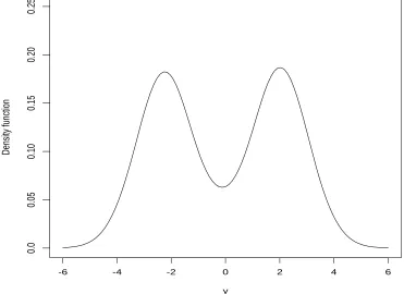
Figure 2.1, the true density is a mixture of normal distributions with the form 0.3n(y;−4,1)+ 0.7n(y; 3,1), where n(y;m, v) is the normal density with mean m and variancev. We try to use a general SNP density f₂(y;µ, σ2) for a fixed value K = 2 to approximate the true density, which has the form of

f₂(y;µ, σ2) = (1 +a₁z+a₂z2)2n(y;µ, σ2)/C(a),

where z = (y−µ)/σ, C(a) = 1 +a2

1+ 3a22+ 2a2. More description of general SNP density is given at the end of this section.

Figure 2.1 shows that three possible SNP densities with different estimates of a₁, a₂

and the same estimates of µ = −0.158, σ2 _{= 2}_._{52 might be good. Actually, the density} functionf₂(y;µ, σ2_{) does not change too much and they are visually identical for the pairs} (a₁, a₂) such that max(a₁, a₂)>30 anda₂/a₁ = 2.19. This suggests that the estimation of polynomial coefficients a₁, a₂ using this representation is very unstable.

2.3.2 Representation of SNP Densities

In order to circumvent the difficulty of numerical instability, we propose a

reparameteriza-tion of the coefficients in P_K(z), which is an alternative way to provide a unique represen-tation and contains the special case SNP density given in (2.7). Let

P_K(z) =

K X

|α|=0

(29)

y

Density function

-6 -4 -2 0 2 4 6

0.0

0.05

0.10

0.15

0.20

0.25

0.30

true

a=(2.69, 6.33) a=(10.65, 23.33) a=(85.2, 186.6)

(30)

where

α = (α₁, α₂, . . . , α_q)T

is a multi–index (vector with nonnegative integer elements), and

|α|=

q X

i=1

α_i,

zα =

q Y

i=1

zαi

i .

If we take the proportionality constant in (2.3) equal to 1, then h_K(z) will be unique. It is equivalent to require that

E[P_K2(U)] = 1, (2.8)

where U ∼N(0, I_q).

To have a convenient way to traverse the set {α : 0 ≤ |α| ≤ K}, let the J elements of {α : 0 ≤ |α| ≤ K} be ordered in some arbitrary way and denote that a_α = p_j, Uα ₌ _V

j,

j = 1, . . . , J. Then

P_K(U) =

J X

j=1

p_jV_j =pTV,

where p = (p₁, . . . , p_J)T _and _V _{= (}_V

1, . . . , VJ)T. Thus, for example, with q = 2, so that

U = (U₁, U₂)T_{, and} _K _{= 2,}

(31)

and

V = (1, U₁, U₂, U₁2, U₂2, U₁U₂)T,

corresponding to (2.2). Therefore,

E[P_K2(U)] = E(pTV VTp) =pT{E(V VT)}p=pTAp, (2.9)

where

A= E(V VT),

and is very straightforward to compute since every element is the expectation of the product

of powers of independent standard normal random variables. It is well known that A is a positive definite matrix. Thus it has a decomposition

A=BTB, (2.10)

where B is an upper triangle matrix. Therefore, substituting (2.10) and (2.9) into (2.8), we obtain

(Bp)TBp= 1,

i.e.,

(32)

where c=Bp= (c₁, . . . , c_J)T. Thus, we can use the reparameterization

c₁ = cos(ψ₁)

c₂ = sin(ψ₁) cos(ψ₂) ..

.

c_j = sin(ψ₁) sin(ψ₂)· · ·cos(ψ_j) ..

.

c_J₋₁ = sin(ψ₁) sin(ψ₂)· · ·cos(ψ_J₋₁)

c_J = sin(ψ₁) sin(ψ₂)· · ·sin(ψ_J₋₁),

(2.11)

where ψ_j ∈(−π/2, π/2] for j = 1, . . . , J −1. Thus, with ψ = (ψ₁, . . . , ψ_J₋₁)T,

p=B−1c(ψ), (2.12)

where c(ψ) is a function of ψ satisfying (2.11).

The advantage of using this reparameterization is that it includes (2.7) as a special case

and has broad representation. Also, it will be more stable to estimate the parameters ψ

instead of p.

For example, with K = 2 andq= 1, let p= (p₁, p₂, p₃)T _and _V _{= (1}_{, U, U}2₎T_{. Then}

(33)

Thus

A= E(V VT) = E

      

1 U U2

U U2 _U3

U2 _U3 _U4

       =       

1 0 1

0 1 0

1 0 3

       , B =       

1 0 1

0 1 0

0 0 √2

       ,

B−1 =

      

1 0 −1/√2

0 1 0

0 0 1/√2

       , and

c(ψ) =

      

cosψ₁

sinψ₁cosψ₂

sinψ₁sinψ₂

       .

Therefore, the coefficients in P_K(z) are given by

p=B−1c(ψ) =

      

cosψ₁−sinψ₁sinψ₂/√2 sinψ₁cosψ₂

sinψ₁sinψ₂/√2

       .

(34)

p₃ =√5/5. Thus the SNP density function has the special form of

h₂(z) = ( √

10

5 +

√ 5 5 z)

2_z2_ϕ 1(z).

Ifψ₁ =ψ₂ = 0, thenh₂(z) = ϕ₁(z) will be a standard normal distribution. We thus propose to represent the density of Z as

h_K(z;ψ) = P_K2(z;ψ)ϕ_q(z), (2.13)

where the notation P_K(z;ψ) emphasizes that the polynomial is parameterized in terms of

ψ.

Now, suppose Y = RZ+γ, where R is a (q×q) upper triangular matrix and γ is a

q–vector. Then the density function of Y is straightforward to compute and is given by

f_K(y;δ) = P_K2(z;ψ)n_q(y;γ,Σ), (2.14)

where z = R−1₍_y₋_γ_{), Σ =}_RRT _and _n

q(y;γ,Σ) is a q–variate multinormal density with

mean γ and variance–covariance matrix Σ. The parameters δ are made up of ψ, γ and R. This is the general form of SNP density function we will use.

The shape of general SNP density function f_K(y;δ) is rich enough to approximate a wide range of behaviors. Densities with this representation can be skewed, multi–modal,

(35)

multi–modal, symmetric as well as very skewed.

2.4 Random Sampling from a SNP Density

2.4.1 Acceptance–Rejection Method

Gallant and Tauchen (1992) proposed an algorithm to generate a random sample from a

SNP density. We apply this algorithm for our representation of SNP densities. We first

describe acceptance–rejection methods (Kennedy and Gentle, 1980) for sampling from an

arbitrary density h(z). This depends on finding a positive, integrable function d(z) that dominates h(z), i.e.,

0≤h(z)≤d(z), for any z.

In this case, d(z) is called an upper envelope for h(z) or a majorizing function. Derive a density g(z) from d(z) by normalizing

g(z) = R d(z)

d(s)ds.

Usingd(z) and g(z), a sample z fromh(z) is generated as follows.

1. Generate the pair (u, v) independently, u∼U(0,1), v ∼g(v).

2. If u≤h(v)/d(v) then accept z =v; otherwise, go to 1 and repeat until one sample z

(36)

y

Density function

-6 -4 -2 0 2 4 6

0.0

0.05

0.10

0.15

0.20

0.25

(37)

y

Density function

-6 -4 -2 0 2 4 6

0.0

0.05

0.10

0.15

0.20

0.25

0.30

(38)

y

Density function

-6 -4 -2 0 2 4 6

0.0

0.05

0.10

0.15

0.20

(39)

y

Density function

-6 -4 -2 0 2 4 6

0.0

0.05

0.10

0.15

0.20

(40)

The algorithm can be proved by the following arguments:

Pr(z ≤t) = Pr[{(u, v) :v ≤t}|{(u, v) :u≤h(v)/d(v)}]

= Pr[(u, v) :v ≤t, u≤h(v)/d(v)] Pr[(u, v) :u≤h(v)/d(v)]

=

R v≤t

R_h₍_v₎_/d₍_v₎

0 g(v)dudv

R v≤∞

R_h₍_v₎_/d₍_v₎

0 g(v)dudv =

R

v≤tg(v)h(v)/d(v)dv R

v≤∞g(v)h(v)/d(v)dv

=

R

v≤th(v)dv R

v≤∞h(v)dv

=

Z

v≤t

h(v)dv.

Thus,z generated by the above rejection method is a sample fromh(z).

2.4.2 Sampling from a SNP Density

For our problem, we need to find an upper enveloped_K(z) for SNP densityh_K(z). We have

h_K(z) = P_K2(z;ψ)ϕ_q(z),

and

P_K(z;ψ) =

K X

|α|=0

(41)

Note that the coefficient a_α inP_K(z;ψ) is a function ofψ, for {α: 0≤ |α| ≤K}, which is defined in (2.12). Since

K X

|α|=0

a_αzα ≤

K X

|α|=0

|a_α||z|α,

where |z|denotes the vector z with each element replaced by its absolute value,

d_K(z) =

  

K X

|α|=0

|a_α||z|α

  

2

ϕ_q(z)

is an upper envelope for h_K(z), and the densityg_K(z) is given by

g_K(z) = R dK(z)

d_K(s)ds.

To obtain the density g_K(z), note that

d_K(z) =

K X

|α|=0

K X

|γ|=0

|a_α||a_γ||z|α+γϕ_q(z)

=

K X

|α|=0

K X

|γ|=0

|a_α||a_γ|

(√2π)q ( _q

Y

i=1

|z_i|αi+γi_e−z_i2/2

)

=

K X

|α|=0

K X

|γ|=0

|a_α||a_γ|

(√2π)q ( _q

Y

i=1

Γ[(α_i+γ_i+ 1)/2]2(αi+γi+1)/2−1

)

( _q Y

i=1

χ(|z_i|;α_i +γ_i+ 1)

(42)

is the weighted sum ofChidensity functions (Monahan, 1987), where theChidensity with

ν degrees of freedom is given by

χ(s;ν) = 2 1−ν/2 Γ(ν/2)s

ν−1_e−s2/2_,

for s >0. Thus we can obtain the density

g_K(z) =

K X

|α|=0

K X

|γ|=0

ω_αγ

q Y

i=1

χ(|z_i|;α_i+γ_i+ 1),

where

ω_αγ = |aα||aγ|

Q_q

i=1Γ[(αi+γi+ 1)/2]2(αi+γi+1)/2−1

P_K

|α|=0

P_K

|γ|=0|aα||aγ| Q_q

i=1Γ[(αi+γi+ 1)/2]2(αi+γi+1)/2−1

.

In order to sample fromg_K(z), we need to obtain a sample (α, γ) from the setF(α, γ) = {(α, γ) : 0 ≤ |α| ≤ K,0 ≤ |γ| ≤ K}. This can be done as follows. Let the elements of

F(α, γ) be ordered in an arbitrary way so that it can be indexed by the sequence (α, γ)_j, wherej = 0,1, . . . , J. Letω_j =ω_αγ where (α, γ) = (α, γ)_j. Generateu∼U(0,1). Find the largestL such thatPL_j₌₀ω_j ≤u. Then let (α, γ) = (α, γ)_L. For this given (α, γ), generate

z_i from χ(z_i;α_i+γ_i+ 1) for all i = 1, . . . , q. Then change the sign of z_i with probability 1/2. That is, change the sign of z_i if u₁ ≤1/2; otherwise, do not change it, where u₁ is a random sample from the uniform (0, 1) distribution. Thenz = (z₁, z₂, . . . , z_q)T _{is a sample}

(43)

2. For the given (α, γ), sample z from g_K(z).

3. GenerateufromU(0,1) independently. Ifu≤h_K(z)/b_K(z), then acceptz; otherwise, go to 1 and repeat until one sample point is obtained.

If we wish to obtain a sample y from (2.14), we can generate a sample z from h_K(z) first. Then y=Rz+γ is a random sample fromf_K(y).

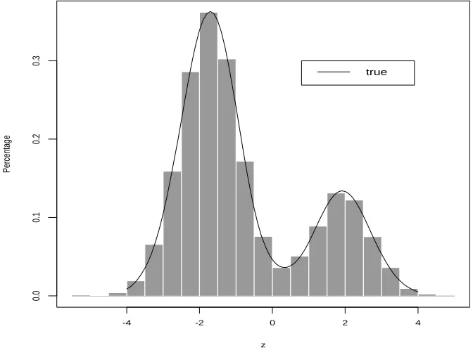
Here we show an example to illustrate the performance of this algorithm. For K = 2 and q = 1,

h₂(z) = P₂2(z;ψ)ϕ₁(z),

where P₂(z;ψ) = a₀+a₁z+a₂z2_, _ϕ

1(z) is the standard normal distribution density. Let

ψ = (−0.7,−1.2). Then we can obtaina= (0.340270,−0.233437,0.424572) by using (2.12). For this example, the rejection algorithm above works efficiently and achieves an acceptance

rate of about 70%. We generated 15000 sample points from this SNP density. Figure 2.6

is the histogram of these 15000 sample points and the true density function. The shape

of histogram matches perfectly to the true SNP density, which shows that this algorithm

works very well and that the sample generated by the algorithm really arises from the true

(44)

-4 -2 0 2 4

0.0

0.1

0.2

0.3

z

Percentage

true

(45)

Chapter 3 Monte Carlo EM Algorithm

3.1 Introduction

If we are willing to assume the response of interest follows some distributional model, the

likelihood method is usually a good way to estimate the parameters which specify the

dis-tributions. However, the likelihood function is not easy to obtain for some complicated

problems like generalized linear mixed models even with normal random effects, which

involves the integration over the random effects. One way to avoid the difficulty of

integra-tion is to use the EM algorithm and treat the random effects as “missing” data. However

we have the same difficulty at the E–step in the generalized linear mixed model context,

because the E–step involves an intractable integral. Some methods were developed by

us-ing Monte Carlo approximation to the required integration at the E–step. The resultus-ing

(46)

3.2 Monte Carlo EM Algorithms

3.2.1 Motivation

In models such as the generalized linear mixed model, the likelihood is of the form

L(ζ;y) =

Z

f(y|b;β, φ)f(b;δ)db. (3.1)

To avoid the difficulty of integration, one clever way is to use the EM algorithm and treat

the random effects b as “missing” data, and y as “observed” data (e.g. Searle et al., 1992, Chap. 8). Then the “complete” data (y, b) have the joint density function f(y, b;ζ) which is the same as the integrand in (3.1). Given the rth iterate estimate ζ(r), at the (r+ 1)th iteration, the E–step involves the calculation of

Q(ζ|ζ(r)) = E{logf(y, b;ζ)|y;ζ(r)}=

Z

logf(y, b;ζ)f(b|y;ζ(r))db, (3.2)

where f(b|y;ζ(r)_{) is the conditional distribution of} _b _given _y_{. The M–step consists of} maximizing Q(ζ|ζ(r)_{) with respect to} _ζ _{to yield the new update} _ζ(r+1)_{. The process is} iterated from a starting valueζ(0) _{to convergence; under regularity conditions, the value at} convergence maximizes the likelihood function (3.1).

Obtaining a closed form expression for (3.2) is often not possible, as it requires

(47)

knowledge of the marginal likelihood whose direct calculation is to be avoided. In

or-der to circumvent this difficulty, much effort (Wei and Tanner, 1990; McCulloch, 1997;

Booth and Hobert, 1999) has been made to use a Monte Carlo approximation to the

re-quired integration at the E–step. Specifically, if it is possible to obtain a random sample

(b(1), b(2), . . . , b(L))T from f(b|y;ζ(r)), then (3.2) may be approximated by at the (r+ 1)th iteration

Q_L(ζ|ζ(r)) = 1

L

L X

l=1

logf(y, b(l);ζ), (3.3)

yielding a so–called Monte Carlo EM (MCEM) algorithm. By independence, to obtain a

sample from f(b|y;ζ(r)_{), one may sample from the conditional distribution of} _b

i given yi

evaluated at ζ(r)_,_f₍_b

i|yi;ζ(r)), say, for eachi.

Incorporating the Monte Carlo approximation into the EM algorithm gives an MCEM

algorithm as follows.

1. Choose starting values ζ(0)_{. Set} _r_{= 0.}

2. At iteration (r+ 1), generate b(l) _from_f₍_b_|_y_;_ζ(r)_),_l _{= 1}_{, . . . , L}_.

3. Using the approximation (3.3), obtain ζ(r+1) _{by maximizing}_Q

L(ζ|ζ(r)).

4. If convergence is achieved, set ζ(r+1) _{to be the maximum likelihood estimate} _ζb_; oth-erwise, set r=r+ 1 and return to 2.

To complete the MCEM algorithm, we need to know how to generate such random

(48)

algorithm (McCulloch, 1997) and rejection sampling scheme (Booth and Hobert, 1999).

3.2.2 Metropolis–Hastings Algorithm

McCulloch (1997) proposed using the Metropolis–Hastings algorithm (Tanner, 1993) to

pro-duce a Markov chain from the conditional distribution of b_i|y_i. To specify the Metropolis– Hastings algorithm, it is important to specify the candidate distribution and calculate the

acceptance function at each iteration. If we choose the marginal distribution of random

effect b_i, f(b_i;δ(r)_{), as the candidate distribution at the} _r_{th iteration, then the acceptance} function takes a neat form. Suppose b_i is the previous draw from the conditional density

f(b_i|y_i;ζ(r)_{) and we generate a new value} _b∗

i from the candidate distribution f(bi;δ(r)).

Then, we accept b∗_i as a sample point from the conditional distribution with probability

A(b_i, b∗_i); otherwise, we retain b_i, and A(b_i, b∗_i) is given by

A(b_i, b∗_i) = min

½

1,f(b

∗

i|yi;ζ(r))f(bi;δ(r))

f(b_i|y_i;ζ(r)₎_f₍_b∗

i;δ(r)) ¾

= min

½

1,f(b

∗

i, yi;ζ(r))f(bi;δ(r))

f(b_i, y_i;ζ(r)₎_f₍_b∗

i;δ(r)) ¾

= min

½

1,f(yi|b

∗

i;ζ(r))

f(y_i|b_i;ζ(r)₎

¾

= min

(

1,

Q_n_i

j=1f(yij|b∗i;ζ(r)) Q_n_i

j=1f(yij|bi;ζ(r)) )

.

(49)

2. Generate a random sample u ∼ U(0,1) independently and take the new value as

bnew_i =b∗_i if u≤A(b_i, b∗_i); otherwise, bnew_i =b_i, where b_i is the previous draw in the Markov chain.

3.2.3 Rejection Sampling Scheme

Alternatively, Booth and Hobert (1999) proposed using a rejection sampling scheme (Geweke,

1996) to generate random samples from the conditional distributionf(b_i|y_i;ζ(r)_{). A random} sample from f(b_i|y_i;ζ(r)_{) can be obtained as follows.}

1. Generate a random sample b∗_i from f(b_i;δ(r)_).

2. Sample u∼ U(0,1) independently. If u≤f(y_i|b∗_i;ζ(r)₎_/τ

i, accept bi =b∗i; otherwise,

return 1 and repeat until a sample b_i is obtained,

where τ_i = sup_b_if(y_i|b_i;ζ(r)_{). Note that}

Pr(b_i ≤t) = Pr[{(b_i∗, u) :b∗_i ≤t}|{(b_i∗, u) :u≤f(y_i|b∗_i;ζ(r))/τ_i}] = Pr[(b

∗

i, u) :b∗i ≤t, u≤f(yi|b∗i;ζ(r))/τi]

Pr[(b∗_i, u) :u≤f(y_i|b∗_i;ζ(r)₎_/τ

i]

=

R b∗_i≤t

R_f₍_y_i_|_b∗

i;ζ(r))/τi

0 f(b∗i;δ(r))dudb∗i R

b∗_i≤∞

R_f₍_y_i_|_b∗

i;ζ(r))/τi

0 f(b∗i;δ(r))dudb∗i

=

R

b∗_i≤tf(yi|b∗i;ζ(r))f(b∗i;δ(r))db∗i R

b∗_i≤∞f(yi|b∗i;ζ(r))f(b∗i;δ(r))db∗i

=

R

b∗_i≤tf(yi, b∗i;ζ(r))db∗i

f(y_i;ζ(r)₎ =

Z

(50)

Therefore,b_i generated by the rejection sampling scheme is indeed a random sample from

f(b_i|y_i;ζ(r)).

3.3 Monte Carlo Error

Unlike the Metropolis–Hastings approach in which the random samples generated in the

Markov chain are dependent, the rejection sampling scheme produces independent and

identically distributed random samples that may be used to assess Monte Carlo error at

each iteration of the MCEM algorithm and hence suggest a rule for changing the sample

size L to enhance speed.

Suppose (b(1)_{, b}(2)_{, . . . , b}(L)_{) is a random sample generated from} _f₍_b_|_y_;_ζ(r)_{) using the} rejection sampling scheme. Let

Q(1)(ζ|ζ(r)) = ∂

∂ζQ(ζ|ζ

(r)₎_,

Q(2)(ζ|ζ(r)) = ∂ 2

∂ζ∂ζTQ(ζ|ζ

(r)₎_,

and define Q(1)_L (ζ|ζ(r)_{) and} _Q(2)

L (ζ|ζ(r)) similarly, where

Q(ζ|ζ(r)) = E{logf(y, b;ζ)|y;ζ(r)},

and

Q (ζ|ζ(r)) = 1

L X

(51)

Now, suppose we obtain ζ(r+1) and ζ∗(r+1) by maximizing Q_L(ζ|ζ(r)) and Q(ζ|ζ(r)) respec-tively, i.e.,

Q(1)_L (ζ(r+1)|ζ(r)) = 0,

and

Q(1)(ζ∗(r+1)|ζ(r)) = 0.

Combining with first order Taylor series expansion, we have

0 = Q(1)_L (ζ(r+1)|ζ(r))

≈ Q(1)_L (ζ∗(r+1)|ζ(r)) +Q(2)_L (ζ∗(r+1)|ζ(r))(ζ(r+1)−ζ∗(r+1)).

Thus,

(ζ(r+1)−ζ∗(r+1))≈ {−Q(2)_L (ζ∗(r+1)|ζ(r))}−1Q(1)_L (ζ∗(r+1)|ζ(r)),

and

√

L(ζ(r+1)−ζ∗(r+1))≈ {−Q(2)_L (ζ∗(r+1)|ζ(r))}−1{√LQ(1)_L (ζ∗(r+1)|ζ(r))}.

Since (b(1), b(2), . . . , b(L)) are i.i.d. from f(b|y;ζ(r)), by the weak law of large numbers (Lehmann, 1998, Sec. 2.1), we have

−Q(2)_L (ζ∗(r+1)|ζ(r)) = −1

L

L X

l=1

∂2

∂ζ∂ζT logf(y, b

(l)_;_ζ∗(r+1)₎ → E

½

− ∂2

∂ζ∂ζT logf(y, b;ζ

∗(r+1)₎_|_y_;_ζ(r)

¾

(52)

and

√

LQ(1)_L (ζ∗(r+1)|ζ(r)) =√L

( 1 L L X l=1 ∂

∂ζ logf(y, b

(l)_;_ζ∗(r+1)₎

)

.

By the multivariate central limit theorem (Lehmann, 1998, Sec. 5.4), √LQ(1)_L (ζ∗(r+1)|ζ(r)) follows a multivariate normal distribution with mean

E ∂

∂ζ logf(y, b

(1)_;_ζ∗(r+1)_{) =} _Q(1)₍_ζ∗(r+1)_|_ζ(r)_{) = 0}_,

and variance

var

½

∂

∂ζ logf(y, b

(1)_;_ζ∗(r+1)₎

¾

= E

(·

∂

∂ζ logf(y, b

(1)_;_ζ∗(r+1)₎

¸ ·

∂

∂ζ logf(y, b

(1)_;_ζ∗(r+1)₎

¸_T)

= E

(·

∂

∂ζ logf(y, b;ζ

∗(r+1)₎

¸ ·

∂

∂ζ logf(y, b;ζ

∗(r+1)₎

¸T

|y;ζ(r)

)

def

= B(ζ∗(r+1)|ζ(r)).

Thus, by Slutsky’s theorem (Lehmann, 1998, Sec. 5.1), asymptotically,

ζ(r+1) a∼N(ζ∗(r+1), 1 LΛ

(r+1)₎_,

where Λ(r+1) in the Monte Carlo error for ζ(r+1) is given by

(53)

At the (r+ 1)th iteration, we can use Q(2)_L (ζ(r+1)|_ζ(r)_{) and}_B

L(ζ(r+1)|ζ(r)) as estimators for

Q(2)₍_ζ∗(r+1)|_ζ(r)_{) and} _B₍_ζ∗(r+1)|_ζ(r)_{), where}

Q(2)_L (ζ(r+1)|ζ(r)) = 1

L

L X

l=1

∂2

∂ζ∂ζT logf(y, b

(l)_;_ζ(r+1)₎_, _(3.4)

and

B_L(ζ(r+1)|ζ(r)) = 1

L L X l=1 ½ ∂

∂ζ logf(y, b

(l)_;_ζ(r+1)₎

¾

½

∂

∂ζ logf(y, b

(l)_;_ζ(r+1)₎

¾_T

. (3.5)

A sandwich estimator for Λ(r+1)is obtained by substitutingQ(2)_L (ζ(r+1)|ζ(r)) andB_L(ζ(r+1)|ζ(r))

b

Λ(r+1) =

n

Q(2)_L (ζ(r+1)|ζ(r))

o₋₁

B_L(ζ(r+1)|ζ(r))

n

Q(2)_L (ζ(r+1)|ζ(r))

o₋₁

.

With the normal approximation of Monte Carlo error at each iteration of the MCEM

algorithm, an approximate 100(1−α)% confidence ellipsoid forζ∗(r+1) _{can be constructed.} Since

ζ(r+1) a∼N(ζ∗(r+1), 1 LΛb

(r+1)₎_,

we have

½

1

LΛb

(r+1)

¾₋₁_/₂

(54)

and thus

(ζ(r+1)−ζ∗(r+1))T

½

1

LΛb

(r+1)

¾₋₁

(ζ(r+1)−ζ∗(r+1))∼χ2_s,

where s is the number of parameters in ζ. Thus, a 100(1−α)% confidence ellipsoid for

ζ∗(r+1) _{is given by}

(ζ∗(r+1)−ζ(r+1))T

½

1

LΛb

(r+1)

¾₋₁

(ζ∗(r+1)−ζ(r+1))≤χ2_s,₁₋_α.

Booth and Hobert (1999) advocated updating L as follows. If the previous value ζ(r) _is inside of this confidence region, i.e.

(ζ(r)−ζ(r+1))T

½

1

LΛb

(r+1)

¾₋₁

(ζ(r)−ζ(r+1))≤χ2_s,₁₋_α,

they recommended increasing Lby the integer part ofL/k, where k is a positive constant; otherwise, retainL. The choice ofαandkneeds further investigation. They have advocated choosing α = 0.25 andk ∈ {3,4,5}.

Combining the above, the MCEM algorithm, incorporating a rejection sampling scheme,

is as follows.

1. Choose starting values ζ(0) and initial sample sizeL. Set r = 0.

A Monte Carlo EM Algorithm for Generalized Linear Mixed Models with Flexible Random Effects Distribution

Abstract

A MONTE CARLO EM ALGORITHM FOR

GENERALIZED LINEAR MIXED MODELS WITH

FLEXIBLE RANDOM EFFECTS DISTRIBUTION

Biography

Acknowledgments

Table of Contents

List of Tables

List of Figures

Chapter 1

Introduction

1.1

Background

1.1.1

Motivation

1.1.2

Generalized Linear Mixed Models

1.1.3

EM Algorithm

1.2

Literature Review

Chapter 2

Seminonparametric Density

2.1

Introduction

2.2

SNP Models

2.3

Reparameterization

2.3.1

Motivation

2.3.2

Representation of SNP Densities

2.4

Random Sampling from a SNP Density

2.4.1

Acceptance–Rejection Method

2.4.2

Sampling from a SNP Density

Chapter 3

Monte Carlo EM Algorithm

3.1

Introduction

3.2

Monte Carlo EM Algorithms

3.2.1

Motivation

3.2.2

Metropolis–Hastings Algorithm

3.2.3

Rejection Sampling Scheme

3.3

Monte Carlo Error