Minimizing Execution Time in MPI Programs on an
Energy-Constrained, Power-Scalable Cluster
Robert Springer
David K. Lowenthal
Barry Rountree
Dept. of Computer Science, The Univ. of Georgia springer, dkl, [email protected]
Vincent W. Freeh
Dept. of Computer Science, North Carolina State Univ. [email protected]
Abstract
Recently, the high-performance computing community has realized that power is a performance-limiting factor. One reason for this is that supercomputing centers have limited power capacity and machines are starting to hit that limit. In addition, the cost of energy has become increasingly significant, and the heat produced by higher-energy components tends to reduce their reliability. One way to reduce power (and therefore energy) requirements is to use high-performance cluster nodes that are frequency- and voltage-scalable (e.g., AMD-64 processors).
The problem we address in this paper is: given a target program, a power-scalable cluster, and an upper limit for energy consump-tion, choose a schedule (number of nodes and CPU frequency) that simultaneously (1) satisfies an external upper limit for energy con-sumption and (2) minimizes execution time. There are too many schedules for an exhaustive search. Therefore, we find a sched-ule through a novel combination of performance modeling, perfor-mance prediction, and program execution. Using our technique, we are able to find a near-optimal schedule for all of our benchmarks in just a handful of partial program executions.
Categories and Subject Descriptors D.4.8 [Performance]:
Mod-eling and Prediction
General Terms Measurement, Experimentation
Keywords Power, Energy, Modeling, Prediction, MPI
1.
Introduction
Recently, power-aware computing has gained traction in the high-performance computing (HPC) community. There are two primary reasons for this. First, decreasing power consumption leads to greater reliability (temperature decreases and mean time between failures increases) and maintainability. It also has significant sec-ondary benefits because of the corresponding reduction in heat generated, such as lower cooling costs and increased machine den-sity. Even relatively new centers that house large clusters are having trouble staying within power and cooling constraints [27]. Second,
This research was funded in part by a University Partnership award from IBM and NSF grants CCF-0429285, CCF-0429643 and CCF-0234285.
Permission to make digital or hard copies of all or part of this work for personal or classroom use is granted without fee provided that copies are not made or distributed for profit or commercial advantage and that copies bear this notice and the full citation on the first page. To copy otherwise, to republish, to post on servers or to redistribute to lists, requires prior specific permission and/or a fee.
PPoPP’06 March 29–31, 2006, New York, New York, USA. Copyright c2006 ACM 1-59593-189-9/06/0003. . . $5.00.
because HPC applications rarely achieve peak efficiency, much of the power that is used is actually wasted.
As a result, low-power, high-performance clusters, such as BlueGene/L [1], have been developed to satisfy the ever-increasing demand for energy, while maintaining good performance. Blue Gene/L and similar systems solve this problem by utilizing low-power processors. However, since the processors are only designed to use one voltage, the system uses the same amount of energy un-der load, regardless of the characteristics of that load. Our previous work has shown this can be inefficient for some applications [14].
Our research focuses on using power-scalable clusters, which utilize processors that are each frequency and voltage scalable—
i.e., their clock speed and therefore power consumption can be
changed dynamically. In this paper, we refer to the different avail-able frequencies as energy gears. Such clusters can potentially de-liver good energy efficiency because an increase in CPU frequency generally results in a smaller increase in application performance. The reason for this is that the CPU is frequently not the bottleneck resource.
However, while the CPU frequency of a node (in our case, a node is a single processor) can be scaled down to save energy, such scaling primarily saves CPU energy. A much greater savings is possible by simply not using a node; i.e., using only a subset of the available nodes. Hence, given a power-scalable cluster, there are two primary ways to save energy: (1) power down a subset of the nodes, and (2) on the nodes that are actively participating in the computation, scale down the CPU frequency. This paper synthesizes these two approaches.
The problem we address in this paper is: given a target
pro-gram, power-scalable cluster, and an upper limit for energy con-sumption, choose a schedule that simultaneously satisfies the en-ergy limit and minimizes execution time. In this paper the term schedule means a tuple whose first element specifies the number of
nodes to be used; the remaining elements indicate, for each compu-tational phase, the CPU frequency (gear) in which to execute that phase. Because determining the optimal schedule requires (in the worst case) executing all possible schedules, the problem is expo-nential in the number of phases. Hence, the goal of this paper is to determine a near-optimal schedule, while only (partially) executing a given program a small number of times.
estimates of the key parameters using the additional information collected during the executed iterations.
For evaluation, we used a combination of the NAS parallel benchmarks and several synthetic benchmarks. This allows us to give both a real-world evaluation and an exploration of the bounds of the problem space. Using our technique, we are able to find a near-optimal solution in just a handful of partial program tions. For example, for the NAS FT benchmark, by using 11 execu-tions (of just a few iteraexecu-tions), we discovered a schedule that results in a completion time that is within 2.2% of the optimal. An exhaus-tive search would have required execution of over 100 schedules. In addition, the results are promising not just for FT, but also for the other NAS benchmarks and a set of synthetic programs that cover a range of different application characteristics in terms of parallel speedup and memory pressure.
The rest of this paper is organized as follows. Section 2 de-scribes related work. Section 3 discusses our model and algorithm for finding an effective schedule. Section 4 discusses the measured results on our power-scalable cluster. Finally, Section 5 summarizes and describes future work.
2.
Related Work
This section describes some of the closely related research. It di-vides the related work into two broad categories: performance pre-diction and tuning and energy-related research in server/desktop and mobile systems.
2.1 Performance Prediction and Tuning
First, underlying this work is the problem of understanding parallel scalability. The work in [32] focuses on finding MPI operations that cause scalability problems. This is done though both machine learning and statistical analysis. A model for understanding the scalability of a class of task and data parallel programs is presented in [31].
Second, several researchers have addressed various parallel pro-gramming issues by (1) executing programs, (2) taking measure-ments, and then (3) analyzing the results. Perhaps the best known of these is ATLAS [37], which uses the Automated Empirical
Op-timization of Software technique. Essentially, a specialized library
of linear algebra functions is created by executing the library func-tions over several days, with many different compile-time opfunc-tions. The ADAPT system took a similar approach [34]. The ATLAS technique was generalized to other high-performance computing kernels in [38]. Other related techniques include executing a few it-erations of a high-performance application to predict performance across different platforms [39] and executing MPI routines on each new platform to generate the most efficient implementation [11].
This paper borrows several of these general ideas, but differs in several ways. First, the number of executions that our technique can make is limited, because we are not creating a library, but rather running a program that the user wishes to complete as soon as pos-sible. Second, we address the need to understand program scalabil-ity by running a (small) set of iterations of the program and devel-oping time and energy models that encompass both computation and communication.
2.2 Energy-Related Research
Several people have investigated saving energy in server systems. In sites such as hosting centers where there is a sufficiently large number of machines, energy management may become an issue; see [5, 26, 10] for examples of this using commercial workloads and web servers. Such work shows that power and energy man-agement are critical for commercial workloads, especially web servers [22]. Additional approaches have been taken to include dy-namic voltage scaling (DVS) and request batching [9]. The work
in [29] applies real-time techniques to web servers in order to con-serve energy while maintaining quality of service.
Our project differs from most prior research because it fo-cuses on HPC applications and installations, rather than commer-cial ones. An HPC installation exists to speed up an application, which is often highly regular and predictable. One approach is to save energy in an application-specific way; the work in [6] used this approach for a parallel sparse matrix application. Another HPC effort that addresses the memory bottleneck is given in [17]. Also, Cameron et al. [3] use a variety of different DVS scheduling strategies (for example, both with and without application-specific knowledge) to save energy without significantly increasing execu-tion time. None of this work, however, considers finding a schedule. In server farms, disk energy consumption is also significant; several have studied reducing disk energy (e.g., [4, 41, 16, 25]). In this paper, we do not consider disk energy, as it is relatively minor compared to CPU energy, especially if scientific programs operate primarily in core.
There are also a few high-performance computing clusters de-signed with energy in mind. One is BlueGene/L [1], which uses a “system on a chip” to reduce energy. Another is Green Destiny [35], which uses low-power Transmeta nodes. A related approach is the Orion Multisystem machines [24], though these are targeted at desktop users. Unlike our approach, these machines sacrifice per-formance in order to save energy by using less powerful processors. While not our focus in this work, there is also a large body of work in saving energy in mobile systems. At the system level, there is work in trying to make the OS energy-aware through mak-ing energy a first-class resource [8, 7]. One important avenue of application-level research on mobile devices focuses on collabo-ration with the OS [23, 36, 40, 12]. Our approach differs in that we are concerned with saving energy in HPC applications, where execution time is the primary consideration.
Our prior work is threefold: an evaluation-based study that fo-cused on exploring the energy/time tradeoff in the NAS suite [14], development of an algorithm for switching CPU frequency (gear) dynamically between phases [13], and leveraging load imbalance to save energy [20].
In [13], we establish the usefulness of varying the energy gear per phase and providing an algorithm for choosing the gear assign-ment. This paper extends this idea by allowing the number of nodes to vary, which complicates the problem considerably.
Finally, in our work we divide programs into one or more computational phases. There has been a large body of work in phase partitioning. Static techniques, such as [21, 28], appeared in the literature first. More recently, dynamic techniques have been used [19, 30].
3.
Implementation
This section describes our implementation. The inputs to our sys-tem are a program divided into phases, an energy limit, and a maximum number of available nodes. Our system will output a ( )-tuple, or schedule, the first element of which is the num-ber of nodes to use, and the remainder the CPU frequency (energy
gear) selected for each phase. To determine a schedule, we use a
combination of performance modeling and performance prediction, backed up by small number of program executions (where each ex-ecution is only a handful of iterations).
Our system takes as input a program divided into one or more
phases. For this paper, we used a straightforward phase division
Second, if the memory pressure changes abruptly, a block boundary occurs at this point. (Memory pressure is determined by inspecting performance counters; for this paper we look at operations and cache misses.) We have found in previous work that multiple phases are necessary to obtain good time/energy tradeoffs in several of the NAS benchmarks. For example, in MG, by using multiple phases we were able to save an additional 11% energy compared to using a single phase (and therefore only a single gear). Further details are available in [13] and in Section 4.
This section first describes our assumptions in this paper. Then, it presents our time and energy models. Next, we give our algorithm for finding an effective schedule. Finally, we discuss specific details of our algorithm.
3.1 Assumptions
First, the effectiveness of our system relies on having valid parti-tionings of phases. We consider the general phase division problem to be orthogonal to our research, but can leverage off of a large amount of related work in the area (described in Section 2).
Second, we assume that we are given an maximum (total) en-ergy constraint (by the user or cluster administrator). While not currently policy on large supercomputers, based on others’ expe-rience with large clusters in even modern data centers [27], we can envision a situation in the near future where the cost of energy is charged at least partially to the user. This constraint may be im-posed for many reasons; for example, the aggregate mean time to failure of large clusters has fallen into the range of minutes [18]. The Arrhenius equation states that a reduction in operating temperature will result in a doubling of expected hardware life-time [33]. Because energy consumed translates directly into heat dissipated, reducing energy consumption should extend hardware lifetimes.
Third, we assume no load imbalance. In future work we will ad-dress load imbalance, but the programs in the NAS suite generally balance the computation between nodes fairly evenly. Extending the model described in the next subsection to handle load imbal-ance is a nontrivial task. Finally, we assume that program behavior between iterations is consistent, so that it is possible to predict fu-ture program behavior by examining current behavior.
3.2 Model
In this section we describe our models of execution time and con-sumed energy. Later, we discuss the algorithm we use to predict time and energy in as few iterations as possible.
In our previous work [14], we noted that (1) computation time and communication time tend to scale differently as the number of nodes increases, and (2) the power consumed by the system is different when computing than when communicating. Therefore, our model separates execution time and consumed energy into their computation and communication components:
where is computation time and
is the communication time (which we assume is primarily blocking), while and are the corresponding average power consumption levels. Below we show how to model time and energy as a function of the energy gear and the number of nodes; that is, the model produces the functionsand. Given this model, one can estimate the time and energy for all values ofandwith only a handful of empirical measurements. The four individual terms in the model are discussed below.
Computation time To determine the effect the number of nodes
has on , we make use of Amdahl’s law. The computation com-ponent of a program can be decomposed into parallelizable and
inherently serial fractions ( and
, respectively). Given, computation time in the fastest gear (gear 0) as a function ofis:
Now we address the effect the number of gears has on . Let
be the slowdown of the computation at
gearrelative to top gear. Our data indicates that
is independent of. Putting it together,
Both and
are determined experimentally.
Communication time We assume that any time spent in blocking
communication calls is unaffected by gear because the CPU is
mostly idle. In other words, . Using
measurements of
on a handful of different numbers of nodes, we develop an equation to extrapolate
for all(described in the next subsection).
Computation power The model makes two assumptions
regard-ing power consumed durregard-ing computation. First, it leverages the as-sumption of no load imbalance to conclude that each node uses the same amount of power, i.e., . Next, it assumes that per-node power consumption is independent of the total number of nodes. Our previous work has found this is gener-ally true [14]. The exception to this rule occurs when changing the number of nodes causes a material change in the application. One example of this is when an application is out of core on nodes but in core onnodes ( ). (The CG benchmark has this property; see Section 4 for details). In any case, what is needed to find is simply measurements of .
Communication power In order to determine
, we mea-sure , and then, similar to the assumption that communi-cation time is independent of gear, we assume that power while communicating is also independent, i.e., . Therefore,
.
While the above equations are relatively straightforward, there are two situations where they are not fully precise. First, we as-sumed that
and
are independent of the gear. It turns out that they are actually affected by the gear. We further discuss how we extend the model to improve its accuracy in Sec-tion 3.4.
Second, in our earlier work [14], we discussed the effects of
re-ducible time, on execution time when changing gears. Rere-ducible
time is defined as the time between an send/receive or send/wait pair. It is important because when using a lower gears, computation speed slows but communication speed remains relatively constant. Any reducible work increase, therefore, will result in a correspond-ing blocked time () decrease (unless reaches zero).
We analyzed program traces to determine the amount of re-ducible time for the programs considered for these experiments and found that all but one of them had essentially no reducible time.1 Thus, we elected not to consider the effects of reducible time in this paper, but we will consider this in future work.
3.3 Algorithm
Broadly speaking, our algorithm repeatedly executes the program for a handful of iterations. On each run, we measure time and energy as well as refine our estimates for a subset of the dependent variables (,, and ) in our model. This improves our
1The NAS SP benchmark had 6s of reducible time out of 60s of
overall estimate of execution time and energy consumption. This section provides details of our algorithm.
3.3.1 Step 1: Initialize
The first step is to determine initial values for ,, and
. The minimum number of runs to do this is
. The first runs are required to determine for each energy gear. This is done by executing the program on one node and dividing the observed energy consumption by the execution time. One node is used so that communication does not affect our measurements. In other words, we are only measuring computation power. Note that power is not constant over different applications, because their different characteristics lead to different use of the machine.
Combined with the one-node, top gear run, we can create accu-rate estimates for ,
, and, with just two addi-tional runs. These are performed in top gear. To estimate , we use a regression on measured values for. Our previous work has shown that for programs without scaled speedup,
scales lin-early with the number of nodes. Therefore, a linear regression using these values is an accurate way to predict their values at unknown numbers of nodes.
To estimate, we first note that communication time may scale in different ways depending on the implementation of a specific program. In most cases, communication time scales either logarithmically, linearly, or quadratically. Knowing which of these models best fits the communication of a particular program requires three runs. With the observed data, we fit the data to each of the three functions, and select the function that gives the lowest average error.
We found that the best way to predictwas to use micro-ops per data cache miss, OPM. Our previous work shows that OPM cor-relates well with memory pressure [15]. Through experimentation, we found that a logarithmic function best fits the relation between OPM and
. We used this to estimate
for unknown numbers of nodes. The reason we use OPM to indirectly measure
is because is not constant across numbers of nodes; indeed, cache perfor-mance (which is directly related to how much pressure is exerted on memory) often improves when nodes are added.
3.3.2 Step 2: Predict and sort all schedules
Because the time taken to predict execution time and consumed energy (as opposed to executing the program) for a given schedule is negligible, we make predictions for every possible schedule. We divide the schedules into two lists: those predicted to satisfy the energy constraint (denoted satisfying), and the remainder (denoted
non-satisfying). Because the power meter has a limited precision
(see Section 4.2 for details), a schedule is deemed satisfying if the energy consumed is smaller than the difference of the limit and the error.
Each list is then sorted: the satisfying list in order of increasing execution time, and the non-satisfying list in order of increasing energy. In other words, the first schedule on the satisfying list is the one predicted to be fastest within the energy constraint. Further-more, the first schedule on the non-satisfying list is predicted to be closest to satisfying the energy constraint.
3.3.3 Step 3: Execute schedule, update estimates
We then select the first schedule on the satisfying list. In this step we do not ever select a test that was previously executed (see below). We execute this schedule for a few iterations (5 in all of our tests). The results are compared to the energy constraint, and if it indeed is below the constraint, we perform validation tests (step 4). Otherwise, we update our estimates ofand(using regression as in step 1) and return to step 2.
Run Schedule Time Energy
Predicted Actual Predicted Actual
½ (1, [0, 0]) — 267 — 28.0
¾ (4, [0, 0]) — 100 — 38.5
¿ (9, [0, 0]) — 64 — 53.1
1 (4, [2,1]) 108 109 36.9 36.2
2 (4, [1,1]) 107 101 37.6 35.1
G (4, [0,1]) 107 110 37.9 37.1
N (9, [4,4]) 73.2 68.4 47.1 42.5
S (4, [1,1]) 107 101 37.6 35.1
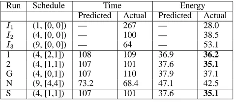
Table 1. An illustration of our algorithm on SP with an energy
limit of 37 kJ. Boldface entries satisfy the energy limit.
3.3.4 Step 4: Validate schedule
Once we have found a schedule that satisfies the energy constraint, we wish to ensure that the proposed solution is close to the best possible schedule. To do this, we run two further tests: one which differs in gear selection, and the other differs in the number of nodes.
To ensure we are using the right gear, we perform what we call
gear validation. We consider a schedule using the same number
of nodes, but with at least one phase using a faster gear. To do this we use the first such schedule on the non-satisfying list. If this schedule does not satisfy the constraint, it means that any schedule using strictly faster gears and the same number of nodes will fail to satisfy the energy constraint.
This schedule is then executed for a few iterations. If this sched-ule does not satisfy the constraint, it means that any schedsched-ule using strictly faster gears and the same number of nodes will fail to satisfy the energy constraint. If the test does satisfy the energy constraint, then we go to step 2 and regenerate new estimates for all schedules. Otherwise, we proceed to node validation, which is similar in spirit to gear validation. Specifically, we examine the non-satisfying list for schedules that use a larger number of nodes than the current schedule.2Of those schedules, we choose the one that is predicted to use the least energy and executes faster than the candidate sched-ule. This schedule is then executed for a few iterations. If it does
not satisfy the energy constraint, it is unlikely that any solution
us-ing more nodes will satisfy the energy constraint or execute in less time.
At this point we have shown that there is likely no better legal schedule if the number of gears or nodes is changed, so our algo-rithm terminates and returns the candidate schedule. Presumably the user will now execute the entire program using this schedule.
On the other hand, if the node validation test does satisfy the constraint, then, as before, it means the candidate solution may be able to be improved with better estimates, and so we return to step 2.
It is possible that a validation test may be skipped: this occurs if either (1) we are using top gear for all phases (so there is no schedule with a faster gear), or (2) we are using the maximum number of nodes (so there is no schedule with more nodes). In either case, that validation test is skipped. In addition, a given schedule is only run once during program execution. We store the results of every execution so that should a schedule be selected twice, the results of the first run will be used.
3.3.5 Example
We illustrate our algorithm for the specific case of SP with an energy limit of 37kJ. Table 1 shows the steps carried out. In the
2The NAS programs do not run on an arbitrary number of nodes, so the
table, the entries in the Run column are one of the following:½,
¾, and ¿ are the initialization tests, an S denotes the accepted schedule, G is a gear validation test, N is a node validation test, and an integer denotes an ordinary test. If the actual energy value is below the limit, then that entry is in bold. A schedule is described by ( , [¼,½, ]), where is the number of nodes and
is the gear to be used for phase.
First, we run the initialization tests on different numbers of nodes (
½ through
¿). (For brevity, we omit the gear-based ini-tialization tests.) Then, we predict energy consumption and exe-cution time for all schedules. Based on the predictions, we select (4, [2,1]) as the the fastest schedule predicted to satisfy the energy constraint. Then, we execute the program using this schedule for a few iterations and collect the energy consumed. Because it is below the energy limit, we attempt the gear validation test, which uses the schedule (4, [1, 1]). This is the schedule that uses the same number of nodes, but at least one faster gear, and is predicted to be faster than (4, [2, 1]) but to consume more energy than the limit. After ex-ecution of this test, we note that, contrary to our predictions, (4, [1, 1]) did satisfy the energy limit. Therefore we refine our estimates, return to step 2, and once again predict all schedules.
This time, the best predicted schedule is (4, [1, 1]) and, because it has already been evaluated, we begin gear validation again. The schedule (4, [0, 1]) is selected and executed. The result is that it does not satisfy the energy limit. Thus gear validation is successful, and we progress to node validation. For this, we select the schedule (9, [4, 4]). This is the schedule with more nodes that is predicted to be closest to, but not satisfying, the limit. Execution of this schedule showed that it did not satisfy the limit, so node validation is successful. This means that the algorithm terminates, returning (4, [1, 1]) as the selected schedule.
3.4 Implementation Details
This section describes some specific details of our implementation. First, we discuss how we collect data. Then we describe how we estimate
.
3.4.1 Data Collection
To initialize the dependent variables (, ,
) of the model, it is necessary to gather data from program executions. To do so, we utilize a combination of MPI call profiling, hardware per-formance counters, and inline multimeters. As described above, we need to collect ,
, and OPM in order to estimate the above dependent variables.
To do this, we use use our MPI-JACK tool, which intercepts MPI calls and allows for arbitrary code to be inserted before and after execution of the call. This was used to gather the duration of each MPI call as well as to inspect the performance counters to obtain micro-operations and cache misses (to determine OPM).
We determine energy consumption by placing a WattsUp wattmeter between the system power supply and the wall; then, Power readings are taken from the multimeter every second. The values are integrated over time to yield energy consumption.
3.4.2 Generalizing
Earlier, we assumed that any time spent blocking on communi-cation calls (e.g., MPI Allgatherand MPI Recv) consumes constant power. Separate results [15] have showed that the time is largely (but not completely) independent of gear. Therefore, we do not concern ourselves with a generalization of
.
However, we found through experiments that the power con-sumed blocking on communication calls could be significantly more than idle power—and that it varied with gear. This is be-cause there is a computation component of communication time (e.g., copying between an MPI buffer and a user buffer) that may be significant. So, it is inaccurate to consider power due to
commu-nication for blocking calls to be identical to power consumed when the system is idle. Because different MPI calls have different com-putation/communication ratios, we need to determine power due to communication separately for each call.
To address this issue, on any multiple-node run we use
MPI-JACK to log all message events. We record the computation
portion of communication routines as well as the energy con-sumed. is determined experimentally. Then, we
deter-mine
at top gear by first using:
To calculate
for an arbitrary gear , we need to know the percentage difference between CPU power consumption for all
. Because represents the combination of CPU and sys-tem power, it is necessary to record syssys-tem-only power by taking readings when idle. Once system power has been measured, the CPU-only power is measured by subtracting the idle power from
. Then,
can then be computed by multiplying
by the CPU power at geardivided by CPU power at top gear.
4.
Performance
This section reports our performance results. For all experiments, we used a 10-node AMD Athlon-64 cluster connected by a 100Mbps network. Each node has 1 GB of main memory. The Athlon-64 CPU supports energy gears of 2.0, 1.8, 1.6, 1.4, 1.2, 1.0, and 0.8 GHz, but the 1.0GHz gear was not reliable and so was not used. Each node runs the Fedora Core 2 OS, and gear shifting was done through thesysfsinterface. All applications were compiled with eithergccor the Intel Fortran compiler, using the-O2 optimiza-tion flag. We controlled the entire cluster, so all experiments were run when the only other processes on the machines were daemons. We first describe the overall results of running the NAS suite [2] on our system. Then we present the results of more detailed examinations of the behavior of both our algorithm and model.
4.1 NAS Parallel Benchmarks
Table 2 displays the results of running the NAS programs on our system. For each program, we selected an energy limit as follows. First, we measured the energy consumed running at top gear (de-noted as gear 0) for all phases, using 8 nodes (or 9, for those bench-marks that require it). Then, we subtracted 10% from this amount of energy. This results in a different energy limit for each applica-tion because the applicaapplica-tions execute for different lengths of time.
In the table, we first show the number of executions incurred by our algorithm (labeled Necessary). Next, we show the number of schedules that could be selected by an optimal algorithm
(Opti-mal). Any other schedule would never be chosen by an optimal
al-gorithm, because it is dominated by a schedule that takes less time
and uses less energy. (There is exactly one optimal schedule for any
given energy limit, but the optimal schedule may change if the limit changes.) The next column shows number of executions needed for an exhaustive search (Exhaustive). Finally, and most importantly, we show the time difference from optimal. The optimal solution was obtained through exhaustive search; of course, in general this is not feasible. Recall that each “execution” is not an execution of the entire program, but rather a small number of iterations (5 in the NAS programs).
Program Energy Limit (kJ) Executions Chosen Schedule Time Difference Necessary Optimal Exhaustive
BT 65 16 18 108 (9, [1,1]) 0.0%
CG 20 12 7 24 (4, [1]) 0.0%
EP 45 11 4 24 None —
FT 72 11 47 144 (8, [4,4]) 2.2%
IS 33 14 16 24 (8, [2]) 0.0%
LU 23 15 36 864 (8, [2,4,2]) 6.1%
MG 21 13 29 144 (8, [2,3]) 2.0%
SP 48 16 15 108 (9, [2,1]) 0.0%
Table 2. Results of running our algorithm on NAS parallel benchmarks. The chosen energy limit is 10% less than the energy consumed at
top gear for all phases, using 8 nodes (or 9, for BT and SP). The time difference is that between executing the program using our chosen schedule and executing the optimal schedule. Note that the “necessary” executions include eight executions required for initialization.
runs ( ¾
, as there are three possible node configurations, six gears, and two phases), this is reasonable—and is the worst case over the entire NAS suite in terms of the number of runs. Note that LU requires 864 runs to complete all permutations, and our system only needs 15 to arrive at a schedule just 6.1% from optimal.
In fact, in some cases we achieved the minimum number of runs: 8 initialization runs and 3 subsequent runs (one prediction and then up to two validation tests). This was the case for EP and FT. It is worth noting that the reason that BT required the most executions is because the energy constraint was in a region containing many clustered schedules (i.e., both their time and energy are similar). Based on the observed accuracy of the BT predictions, it is likely that fewer executions would be needed with a different constraint (we verified this with additional experiments). More details on the effect of the energy limit are given in Section 4.2.
We emphasize that the number of initialization runs remains constant as both the number of available nodes and the number of program phases increase—meaning that the initialization runs will be negligible on large clusters executing large-scale programs. Additionally, if the energy limit is later changed, the initialization runs need not be repeated.
Next, we examine the quality of the chosen schedule. We deem our system to have chosen a high-quality schedule if it results in an execution time that is close to that of the optimal schedule.
Table 2 shows that our system does indeed select a high-quality schedule in all cases. For BT, CG, IS, and SP, our algorithm se-lected the optimal schedule. In the case of FT, the chosen sched-ule produced an execution time that was within 2% of the optimal schedule. The reason we did not select the best schedule is because there are many schedules “near” the chosen schedule in the prob-lem space. In general, this makes choosing the optimal schedule challenging; on the other hand, a suboptimal choice is likely to re-sult in an execution time close to the optimal. In the case of LU, we chose the schedule (8, [2,4,2]). Nevertheless, this is our worst case and is only 6% from optimal. It is important to note that by soften-ing the constraints in our algorithm for what schedules should be accepted, we could explore more of the search space and arrive at a better result. However, the cost would be more program executions for all programs, and our system finds a near-optimal schedule in all other cases.
Additionally, in EP no schedule satisfied the 10% energy limit. For this program, 8 nodes at top gear consumes 50kJ, so the energy limit chosen was 45kJ. Because EP gets nearly perfect speedup, the energy consumption is essentially the same on all node configura-tions, because the time decreases as nodes are added. Also, EP is highly CPU bound. Therefore, reducing the gear has a large time penalty and little energy savings.
Finally, CG is an interesting case. This application presented a potential problem for our system because on our cluster, the one-node program is out of core. This results in superlinear speedup for
17 18 19 20 21 22 23 24 25 26
20 40 60 80 100 120 140 160 180
Energy (KJ)
Time (s) 8 nodes
4 nodes
2 nodes Multiphase Single phase Dominating
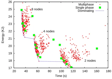
Figure 1. Energy-time scatter plot of every LU schedule.
Sched-ules on the line are not dominated. For readability, the axes do not start at the origin.
the two-, four-, and eight-node programs and results in distorted values of. This in turn can cause the gear and node validation steps to fail because a better schedule arises.
To handle CG, we used a simple filtering technique to remove anomalous results. Specifically, when our system detects superlin-ear speedup, we compute
using the first number of nodes that re-sults in an in-core program. This allowed our system to choose the optimal schedule, which was (4, [1]). Separate tests showed that without filtering, the schedule chosen was (2, [0]), which would have resulted in a 10% slowdown in time as well as two extra exe-cutions.
4.2 Detailed Results
In this section, we examine in more detail several aspects of our model as well as the behavior of our algorithm. Specifically, we first examine our assumption that using different gears in different phases is important. Then, we investigate the behavior at the ex-tremes of the problem space, the sources of error, the effect of the choice of energy limit, and the accuracy of our predictions,
4.2.1 Multigear schedules
This work is motivated by the notion that a program has phases with different optimal gears. This section presents some empirical data to support this conjecture. First, it looks at LU in detail, then it shows data for all multiphase benchmarks.
Number of schedules Total Optimal Multigear
BT 72 18 13 72%
FT 108 47 36 77%
LU 648 36 35 97%
MG 108 29 20 69%
SP 72 15 11 73%
Table 3. Total schedules (excluding one-node), number of
sched-ules that are not dominated, and the number and percentage of such schedules that are multigear.
Importantly, if only single gear schedules are considered, then ex-ecution time may be much higher. For example, if the energy limit were 22kJ, there are several 8-node multigear schedules that exe-cute in less than 40 seconds. However, the best single-gear schedule under the limit is (4, [0,0]), which takes nearly 60 seconds.
Table 3 shows the overall benefit of using multiple gears on the 5 multiphase NAS benchmarks. The total number of schedules depends on the number of phases, gears, and node configurations, as stated above. Each of these schedules was executed on our cluster. Next, the table shows the number of schedules that are not dominated as well as how many of those schedules are multigear. For NAS, on average, 79% of the schedules that are not dominated are multigear, which we believe shows that a model that allows different gears in different phases is important.
4.2.2 Examining the problem space
In our previous work [14], we showed that the behavior of a par-allel program at different gear settings was dependent on program speedup and memory pressure. The better the speedup, the lower the energy premium to run using more nodes. At the limit, if speedup is perfect, then there is no additional energy cost because doubling the nodes halves the execution time. Also, the higher the memory pressure, the greater benefit in running at a lower gear, be-cause the CPU spends a large amount of time waiting on memory. Together, these two factors control the behavior of a program as it relates to our algorithm and model.
To illustrate that our algorithm can support an arbitrary combi-nation of speedup and memory pressure, we constructed a set of six benchmarks. Each consists of two phases. A phase has (1) ei-ther poor or excellent speedup and (2) eiei-ther low or high memory pressure. Assuming we do not care about order and that we want each phase to have different characteristics, this yields six bench-marks. The idea is that these benchmarks are at the extremes of the problem space, and all NAS benchmarks are in the “interior” of the space.
The results of the six benchmarks, each using three different energy limits, are presented in Table 4. The energy limits are chosen by calculating the value, for each program, of 95% of energy consumed by the 8-, 4-, and 2-node versions at top gear for both phases. There are several interesting aspects of these results. First, our system often finds the optimal schedule (12 times out of 15). Second, when we do not find the optimal, we are always within 6%. Third, the schedule (8, [2,0]) is chosen on all three energy limits for the fifth benchmark, which has excellent speedup in both phases. This is the case because perfect speedup means that adding extra nodes does not increase the energy limit. In addition, top gear is not chosen in the first phase because memory pressure is high. Fourth, most of the schedules chosen have different gears per phase. Last, all schedules shown in Table 4 use the top three gears. This is due to the limits used; different limits will select schedules with slower gears (as occurred in the NAS programs).
0 2 4 6 8 10 12 14 16
14000 16000 18000 20000 22000 24000
Number of runs
Energy limit
0 1 2 3 4 5 6
14000 16000 18000 20000 22000 24000
Percent difference from optimal
Energy limit
Figure 2. Effect of the energy limit. On the top, the number of
executions required. On the bottom, the percentage difference from the optimal schedule.
4.2.3 Sources of error
Here we examine the sources of error in our system. First, we use an external power meter, which is accessed through the serial inter-face. We found that there is a relatively small variation in measure-ments of consumed energy. We believe this is a combination of the precision of the meter and that it is accessed through the serial port. Consequently, very small measurements of energy may be unreli-able. Considering that a typical NAS program consumes thousands of joules even when running for only a handful of seconds, and in-specting how long our programs run, we estimate the meter error to be less than 1%.
Second, as mentioned earlier, we model idle time assuming that it is independent of gear. As idle time includes blocking commu-nication calls, this is not strictly true. However, our measurements have shown that the time to receive data in MPI is relatively insen-sitive to gear. We have not yet measured the precise error here, but our initial results suggest that it is quite small.
4.2.4 Effect of energy limit
In our NAS programs, we chose an energy limit that was 10% less than the peak energy that each program consumed. Here, we inves-tigate the effect of varying the energy limit for a one-phase syn-thetic benchmark that has poor speedup and high memory pres-sure. We vary the limit from 13kJ, which for this program is the minimum needed to find a valid schedule, to 25kJ, where the cho-sen schedule is to use the maximum number of nodes at the fastest gear.
Program Chosen Schedules
95% of 8 Time Diff. 95% of 4 Time Diff. 95% of 2 Time Diff.
(Poor/High, Excellent/High) (8, [2,1]) 3.7% (4, [1,1]) 0.0% None —
(Poor/High, Poor/Low) (8, [1,2]) 0.0% (4, [1,2]) 0.0% (2, [2,0]) 0.0%
(Poor/High, Excellent/Low) (8, [2,1]) 0.0% (4, [1,1]) 0.0% None —
(Excellent/High, Poor/Low) (8, [2,1]) 5.1% (4, [0,1]) 0.0% (2, [2,1]) 0.0% (Excellent/High, Excellent/Low) (8, [2,0]) 0.0% (8, [2,0]) 0.0% (8, [2,0]) 0.0%
(Poor/Low, Excellent/Low) (8, [2,0]) 3.7% (2, [0,0]) 0.0% None —
Table 4. Results of running our algorithm on six synthetic benchmarks. Each program is two phases. For example, (Poor/High,
Excel-lent/Low) indicates that the first phase had poor speedup and high memory pressure, and the second phase had excellent speedup and low memory pressure. Each of the six programs is run with three energy limits (95% of energy consumed by the 8-, 4-, and 2-node programs at top gear for both phases). Note that the number of executions for an exhaustive for all programs is 144. The average number of executions of a program (over all 18 experiments) was 13—2 more than the minimum.
0 5 10 15 20 25 30
0 20 40 60 80 100 120 140 160 180
Energy consumption (kJ)
Execution time (s)
2 nodes 4 nodes 8 nodes
(a) Predicted
0 5 10 15 20 25 30
0 20 40 60 80 100 120 140 160 180
Energy consumption (kJ)
Execution time (s)
2 nodes 4 nodes 8 nodes
(b) Actual
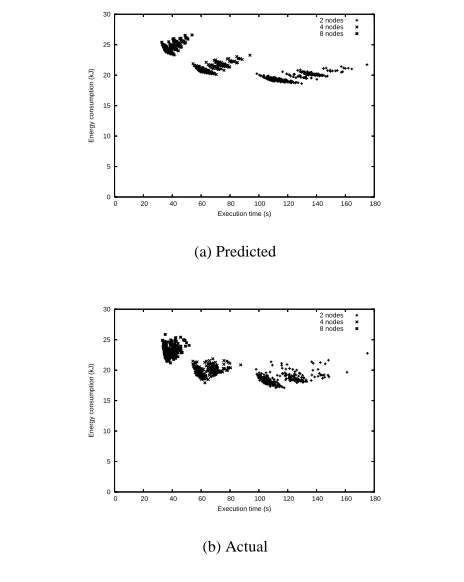
Figure 3. Comparison of predictions vs. actual executions for LU.
(or vice versa). This causes “nearby” schedules to be evaluated. Second, at 18.5kJ, our system produces a schedule that has the largest difference from optimal.
4.2.5 Accuracy of our model
In Table 2 we presented the performance of our algorithm com-bined with our model. The reason we are able to generate near-optimal schedules in few executions is because our model is accu-rate. To examine this further, we used our time and energy model to make predictions for all possible permutations of gears per phase (this totals 864 complete executions) on LU. Then we ran all pro-grams, producing exhaustive results (as described above). The re-sults are presented in Figure 3. Examining the predicted rere-sults, distinct clusters can be seen, one for each number of nodes, and the shapes are similar.
5.
Conclusion
This paper addresses the problem of finding a schedule that mini-mizes execution time on a power-scalable cluster and a maximum energy budget. Our approach uses a combination of performance prediction and profiling, backed up by actual program execution. Results show that typically, only a handful of iterations of a given program need to be executed to find a schedule that results in a near-optimal execution time. In particular, over all NAS benchmarks, typically less than 15 executions (of just a few iterations each) are needed to choose a schedule. Equally importantly, the quality of the chosen schedule is in the worst case 6.1% of the optimal schedule that is found by running all schedules exhaustively. Furthermore, the difference is usually less than 2% of optimal.
While we are encouraged by our results, there are still open questions that we intend to address in future work. First, we hope to implement our system on a much larger cluster. This will help us determine the robustness of our system. Second, we would like to relax some of the assumptions that we have made in this paper; in particular, we would like to expand our model to include load imbalance as well as reducible work. Finally, we plan to use the infrastructure created in this work within a general power-aware MPI runtime system.
References
[1] N.D. Adiga et al. An overview of the BlueGene/L supercomputer. In
Supercomputing, November 2002.
[2] D. Bailey, J. Barton, T. Lasinski, and H. Simon. The NAS parallel benchmarks. RNR-91-002, NASA Ames Research Center, August 1991.
[3] K.W. Cameron, X. Feng, and R. Ge. Performance-constrained, distributed dvs scheduling for scientific applications on power-aware clusters. In Supercomputing (to appear), November 2005.
[4] Enrique V. Carrera, Eduardo Pinheiro, and Ricardo Bianchini. Conserving disk energy in network servers. In Intl. Conference
on Supercomputing, June 2003.
[5] Jeffrey S. Chase, Darrell C. Anderson, Prachi N. Thakar, Amin Vahdat, and Ronald P. Doyle. Managing energy and server resources in hosting centres. In Symposium on Operating Systems Principles, 2001.
[6] Guilin Chen, Konrad Malkowski, Mahmut Kandemir, and Padma Raghavan. Reducing power with performance contraints for parallel sparse applications. In Workshop on High-Performance, Power-Aware
Computing, April 2005.
[7] Compaq Computer Corporation, Intel Corporation, Microsoft Corporation, Phoenix Technologies Ltd., and Toshiba Corporation. Advanced configuration and power interface specification, revision 2.0. July 2000.
Workshop on Hot Topics in Operating Systems, Mar 1999.
[9] Elmootazbellah Elnozahy, Michael Kistler, and Ramakrishnan Rajamony. Energy conservation policies for web servers. In Usenix
Symposium on Internet Technologies and Systems, 2003.
[10] E.N. (Mootaz) Elnozahy, Michael Kistler, and Ramakrishnan Rajamony. Energy-efficient server clusters. In Workshop on Mobile
Computing Systems and Applications, Feb 2002.
[11] Ahmad Faraj and Xin Yuan. Automatic generation and tuning of MPI collective communication routines. In Intl. Conference on
Supercomputing, June 2005.
[12] J. Flinn and M. Satyanarayanan. Powerscope: A tool for profiling the energy usage of mobile applications. In IEEE Workshop on Mobile
Computing Systems and Applications, February 1999.
[13] Vincent W. Freeh, David K. Lowenthal, Feng Pan, and Nandani Kappiah. Using multiple energy gears in MPI programs on a power-scalable cluster. In Principles and Practices of Parallel Programming, June 2005.
[14] Vincent W. Freeh, David K. Lowenthal, Rob Springer, Feng Pan, and Nandani Kappiah. Exploring the energy-time tradeoff in MPI programs on a power-scalable cluster. In International Parallel and
Distributed Processing Symposium, April 2005.
[15] Vincent W. Freeh, Feng Pan, David K. Lowenthal, Nandini Kappiah, Rob Springer, Barry Rountree, and Mark E. Femal. Analyzing the energy-time tradeoff in high-performance computing applications. Submitted to Transactions on Parallel and Distributed Systems, 2005.
[16] Chris Gniady, Y. Charlie Hu, and Yung-Hsiang Lu. Program counter based techniques for dynamic power management. In
High-Performance Computer Architecture, February 2004.
[17] C-H. Hsu and U. Kremer. The design, implementation, and evaluation of a compiler algorithm for CPU energy reduction. In Programming
Languages, Design, and Implementation, June 2003.
[18] Chung-Hsing Hsu and Wu-chun Feng. Towards efficient super-computing: Choosing the right efficiency metric. In Workshop on
High-Performance, Power-Aware Computing, April 2005.
[19] M. Huang, J. Renau, and J. Torellas. Positional adaptation of processors: Application to energy reduction. In International
Symposium on Computer Architecture, June 2003.
[20] Nandani Kappiah, Vincent W. Freeh, and David K. Lowenthal. Just in time dynamic voltage scaling: Exploiting inter-node slack to save energy in MPI programs. In Supercomputing (to appear), November 2005.
[21] Ken Kennedy and Ulrich Kremer. Automatic data layout for distributed-memory machines. ACM Transactions on Programming
Languages and Systems, 20(4):869–916, 1998.
[22] Charles Lefurgy, Karthick Rajamani, Freeman Rawson, Wes Felter, Michael Kistler, and Tom W. Keller. Energy management for commerical servers. IEEE Computer, pages 39–48, December 2003.
[23] Robert J. Minerick, Vincent W. Freeh, and Peter M. Kogge. Dynamic power management using feedback. In Workshop on Compilers and
Operating Systems for Low Power, Charlottesville, Va, September
2002.
[24] Orion Multisystems. http://www.orionmulti.com/.
[25] Athanasios E. Papathanasiou and Michael L. Scott. Energy efficiency through burstiness. In Workshop on Mobile Computing Systems and
Applications, October 2003.
[26] Eduardo Pinheiro, Ricardo Bianchini, Enrique V. Carrera, and Taliver Heath. Load balancing and unbalancing for power and performance in cluster-based systems. In Workshop on Compilers and Operating
Systems for Low Power, September 2001.
[27] Thermal management and server density: Critical issues for today’s data center. http://www.rackable.com/Rackable WPaper.pdf, 2004.
[28] Umit Rencuzogullari and Sandhya Dwarkadas. Dynamic adaptation to available resources for parallel computing in an autonomous network of workstations. In Principles and Practice of Parallel
Programming, June 2001.
[29] Vivek Sharma, Arun Thomas, Tarek Abdelzaher, and Kevin Skadron. Power-aware QoS management in web servers. In IEEE Real-Time
Systems Symposium, Cancun, Mexico, December 2003.
[30] Timothy Sherwood, Erez Perelman, Greg Hamerly, and Brad Calder. Automatically characterizing large scale program behavior. In
Architectural Support for Programming Languages and Operating Systems, October 2002.
[31] Jaspal Subhlok and Gary Vondran. Optimal mapping of sequences of data parallel tasks. In Principles and Practice of Parallel
Programming, July 1995.
[32] J. S. Vetter and M.O. McCracken. Statistical scalability analysis of communication operations in distributed applications. In Principles
and Practice of Parallel Programming, June 2001.
[33] R. Viswanath, W. Vijay, A. Watwe, and V. Lebonheur. Thermal performance challenges from silicon to systems. Intel Technology
Journal, Q3 2000.
[34] Michael J. Voss and Rudolf Eigemann. High-level adaptive program optimization with adapt. In Principles and Practices of Parallel
Programming, 2001.
[35] M. Warren, E. Weigle, and W. Feng. High-density computing: A 240-node beowulf in one cubic meter. In Supercomputing, November 2002.
[36] M. Weiser, B. Welch, A. J. Demers, and S. Shenker. Scheduling for reduced CPU energy. In Operating Systems Design and
Implementation, November 1994.
[37] R. Clint Whaley, Antoine Petitet, and Jack J. Dongarra. Automated empirical optimizations of software and the ATLAS project. Parallel
Computing, 27(1–2):3–35, 2001.
[38] R. Clint Whaley and David B. Whalley. Tuning high performance kernels through empirical compilation. In International Conference
on Parallel Processing, June 2005.
[39] Tao Yang, Xiaosong Ma, and Frank Mueller. Predicting parallel applications’ performance across platforms using partial execution. In Supercomputing (to appear), November 2005.
[40] Heng Zeng, Carla S. Ellis, Alvin R. Lebeck, and Amin Vahdat. Currentcy: Unifying policies for resource management. In USENIX
Annual Technical Conference, June 2003.
[41] Qingbo Zhu, Francis M. David, Christo Devaraj, Zhenmin Li, Yuanyuan Zhou, and Pei Cao. Reducing energy consumption of disk storage using power-aware cache management. In High-Performance