Elliptical Copulae with Dynamic Conditional Correlation

(1)

LIU, FENG. ELLIPTICAL COPULAE WITH DYNAMIC CONDITIONAL

COR-RELATION. (Under the direction of Professor Peter Bloomfield).

Knowledge of the joint distribution is crucial for risk measure estimation,

port-folio allocation, derivative pricing, to name but a few problems. The multivariate

normal function, the most commonly used joint distribution, is not sufficient if data

have features of fat-tailed margins and co-extreme movements, which are commonly

found in financial data. More flexible multivariate distributions are needed in order

to address these features. The copula, originated by Sklar (1959) and also called

the dependence function, can be combined with arbitrary marginal distributions to

form various joint distributions. “Conditional copulæ”, proposed by Patton (2002a),

are adopted by several researchers to introduce time-varying dependence beyond the

existing time-varying variance-covariance. All the research thus far is focused on

bi-variate series. How to extend the models to higher dimension is not obvious. In

the financial world, it is essential to develop models for high dimensional data that

do not suffer the “curse of dimension” problem, but are still rich enough to capture

the major data features, such as fat-tailed margins, volatility clustering, time-varying

correlation and tail dependence.

Motivated by Chen et al. (2004), we propose a model of “elliptical copulæ with

(2)

a straightforward way. Combining the good properties of copulæ and DCC models,

our model is especially attractive for high dimensional data. The general ideas of

our model are as follows: each individual series is modelled by its own appropriate

heteroskedasticity model, and standardized residuals are obtained after filtering out

the estimated dynamic variance; then the standardized residuals are monotonically

transformed to new ones as from the same univariate elliptical distribution; finally,

the transformed residuals are used to build the dependence model of elliptical copulæ

with time-varying correlation from the corresponding elliptical DCC models.

Our model is applied to two financial practices: VaR estimation and optimal

port-folio allocation. The impacts of fat-tailed margins, time-varying correlation and tail

dependence are investigated with two hypothetical portfolios. For VaR estimation,

these data features have substantial importance; while for portfolio allocation, the

(3)

by

FENG LIU

A dissertation submitted to the Graduate Faculty of North Carolina State University

in partial satisfaction of the requirements for the Degree of

Doctor of Philosophy

STATISTICS

Raleigh

2006

APPROVED BY:

Dr. John Monahan Dr. Denis Pelletier

Dr. Peter Bloomfield Dr. David Dickey

(4)

(5)

Biography

Feng Liu was born in Jiangxi, China to parents Rongrong Liu and Muqin Zhang in

May, 1979. She graduated with a B.S. of Statistics from the Department of

Mathe-matics, Beijing Normal University, in July, 2001. In August, 2001, she was enrolled

in the Department of Statistics at North Carolina State University and received her

Master of Statistics degree in May, 2003 and Master of Economics degree in May,

(6)

Acknowledgements

I am largely indebted to Prof. Peter Bloomfield, who has been such a great advisor

and mentor to me. His ingenious ideas and profound insight have constantly inspired

me and guided me through the past three years. And his remarkable knowledge of

statistics and finance has been a great source of enlightenment to me. I am especially

grateful for his enormous patience in dealing with all my questions.

My sincere gratitudes also go to other members of my committee. Prof. Denis

Pelletier’s valuable suggestions, such as parameter uncertainty and duration testing,

have made this work more complete; Prof. David Dickey and Prof. John Monahan

both have read my dissertation carefully and provided numerous useful comments

and feedback. I have also learned a lot from the interesting courses that they taught.

It is a pleasure to thank those people that helped me during my time as a graduate

student. Prof. William Swallow and Prof. David Flath have generously given me

the opportunity to acquire a master degree in Economics, which has facilitated me

in understanding my dissertation topic. During my studying in the Department of

Statistics, Terry Byron has been really helpful to smooth out computer-related issues;

while Adrian Blue and Janice Gaddy have assisted us in so many ways. There are

also other faculty members, staff members and fellow graduate students who have

made the past five years an enjoyable journey for me. I feel fortunate to be around

with all of them.

(7)

He is always there listening to me when I am frustrated, helping me out with his

programing skills and so many other things. I have felt his love at each and every

moment during the course of this study. I also owe my deepest gratitude to my

parents, who always love me, believe in me and support me no matter what. I hope

that I will make them proud by my doctorate fulfillment.

Finally, to my coming baby Ben. His company has given me so much joy and

encouragement and his naughty movements let me not feel lonely when I was sitting

in front of the computer alone. This dissertation is completed little by little with his

(8)

List of Figures

3.1 Simulations from the normal andt copulæ. . . 30

3.2 Relationship of tail dependence with DoF and correlation for the t copula. . . 31

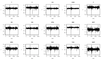
4.1 Graphs of the log returns (yj,t) for each stock. . . 56

4.2 Normal QQ-plots of the residuals j for each stock. . . 61

4.3 Standardized t QQ-plots of the residuals j for each stock. . . 61

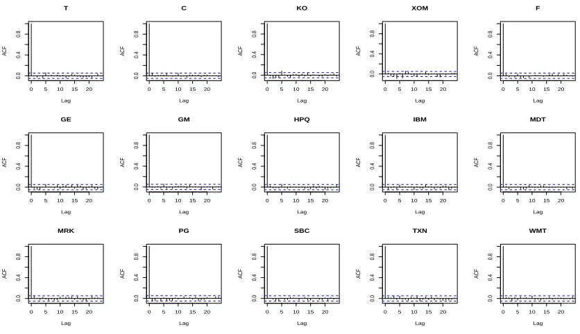
4.4 ACFs of the errorsj for each stock. . . 62

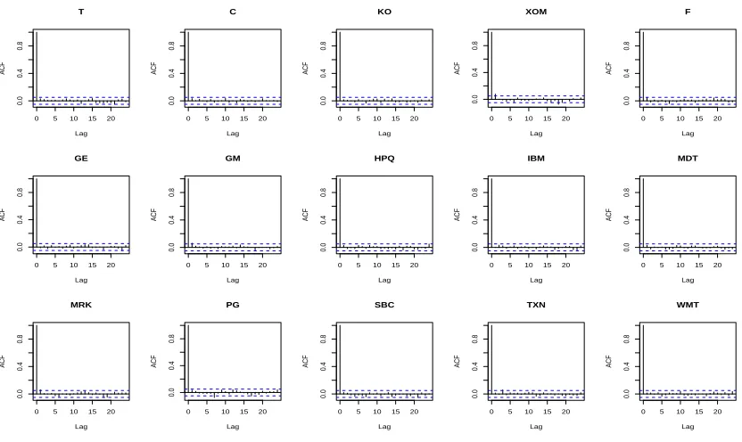
4.5 ACFs of the squared errors 2 j for each stock. . . 63

4.6 ACFs of the residuals ξj for each stock. . . 63

4.7 ACFs of the squared residuals ξ2 j for each stock. . . 64

4.8 1/DoF estimates (1/νˆ) of CTcopulan. . . 69

4.9 1/DoF estimates (1/νˆ) of CTcopulat. . . 69

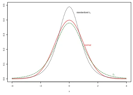
4.10 Graph of the standard normal, standardt5 and standardizedt5density functions. . . 72

4.11 VaRt p estimates for both positions and the corresponding real loss val-ues Lt_{. . . .} ₇₅

5.1 1/DoF estimates (1/νˆ) for the model of CTcopulan. . . 87

5.2 1/DoF estimates (1/νˆ) for the model of CTcopulat. . . 87

5.3 Average utility differences between the EW strategy and some other strategies for short-sale-constrained situation. . . 94

(11)

List of Tables

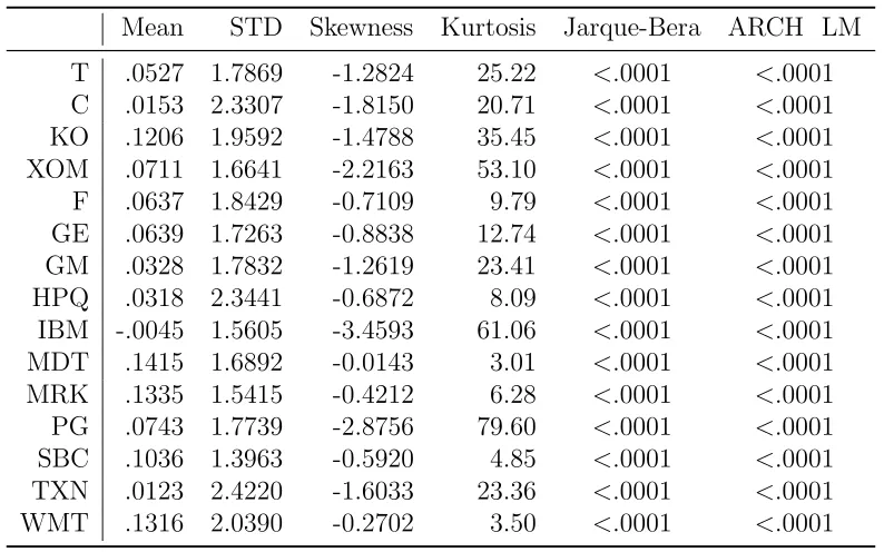
4.1 Summary statistics of the log returns for each stock. . . 57

4.2 2NLL, AIC and BIC of the marginal distributions with the normal or

standardized t residual assumption. . . 59

4.3 The DoF estimate (ˆν) and its corresponding STD of the standardized

t residual distribution for each stock. . . 64

4.4 2NLL, AIC and BIC of the 10 joint distributions for the stock portfolio. 67

4.5 VaR estimates for the stock portfolio. . . 71

4.6 ES estimates for the stock portfolio. . . 73

4.7 The number of violations (N) at different levels for both positions. . . 77

4.8 The backtesting results based on the methods of UC, Markov, CC and

Weibull. . . 79

4.9 The loss function values for some VaR estimation models. . . 82

5.1 Summary statistics of the log-returns for each currency. . . 86

5.2 Summary statistics of the percentage wealth change series for

short-sale-constrained situation. . . 92

5.3 Summary statistics of the percentage wealth change series for

uncon-strained situation. . . 93

5.4 Means of pairwise utility difference and p-values of Wilcoxon signed

rank sum test for short-sale-constrained situation. . . 97

5.5 (Continued) Means of pairwise utility difference and p-values of Wilcoxon

signed rank sum test for short-sale-constrained situation. . . 98

5.6 Means of pairwise utility difference and p-values of Wilcoxon signed

rank sum test for unconstrained situation. . . 99

5.7 (Continued) Means of pairwise utility difference and p-values of Wilcoxon

signed rank sum test for unconstrained situation. . . 100

(12)

Chapter 1 Introduction

This research is motivated by the increasing need for flexible multivariate

distri-butions, especially sound multivariate dependence models. A portfolio’s value-at-risk

(VaR) is determined by the risk behavior of each single asset in the portfolio and, at

the same time, the dependence structure among assets. To set the prices of some

fi-nancial derivatives, like multi-name options, the joint distribution of underlying assets

is needed. Portfolio managers need to obtain information about dependence among

components before making reasonable portfolio allocation decisions. More and more

researchers and practitioners pay attention to the role that dependence between

fi-nancial assets plays in risk management, portfolio allocation and derivative pricing,

to name but a few.

Following Markowitz (1952), the Pearson correlation1 _{coefficient has been widely}

1

(13)

used as the measurement of the dependence among assets. But Cambanis et al. (1981)

identify that correlation is enough to describe dependence only for an elliptic

distri-bution. In order to make problems workable, people often assume the multivariate

normality as the data distribution. As such, the multivariate versions of generalized

autoregressive conditional heteroskedasticity (GARCH) models typically require the

joint residual distribution to be multivariate normal. The normality assumption has

been found to be inappropriate given skewness and leptokurtosis that commonly

ex-ist in financial data even after allowing for the conditional volatility effect (Nelson,

1991). Except for the requirement of univariate normality, the multivariate normal

distribution assumption also imposes tail independence. The co-extreme movement

patterns exhibited by financial assets and markets cannot be captured by correlation,

which, as we noted above, is sufficient to measure dependence only for the multivariate

elliptical distribution. Correlation, as a dependence measure, has some serious

short-comings: a) It is not invariant to monotone transformation; b) It does not incorporate

co-extreme movements in the data; c) Multivariate distributions with identical

cor-relation can have totally different dependence structures. These shortcomings make

correlation not a good measure of dependence outside the elliptical world, especially

when the dependence in the tail areas has non-negligible effects.

One difficulty of modelling multivariate financial series is the scarcity of available

multivariate distributions, which are usually extensions of the univariate distributions

(14)

same probabilistic structure for each asset in the portfolio is unrealistic given its

di-versification purpose. The copula, introduced by Sklar (1959), solves this problem by

constructing multivariate distributions from almost arbitrary univariate distributions

and a chosen dependence structure.

A copula is simply a multivariate distribution with uniform margins. It was first

used explicitly in the financial world in 1999 (Embrechts, et al, 1999; Li, 1999; Ceske

and Hern´andez, 1999). Copulæ enable us to separate the modelling of dependence

from that of margins, which is advantageous considering that, for a portfolio, the

distribution of a single asset may be well studied and different from other assets. As

a result, dependence among multiple series can be flexibly modelled with no influence

on the distribution of each individual series. With special interest to the studies of

risk and portfolio management, copulæ embed information about the entities’

co-movements in the tails of the joint distribution. In the last decade, copulæ have

been heavily studied in areas such as integrated risk management (Hull and White,

1998; Embrechts, et al., 2003; Fortin and Kuzmics, 2002), asset allocation (Patton,

2004; Xu, 2004; Liu, 2005), joint models of credit risk (Li, 2000; Frey, et al., 2001),

multivariate derivative pricing (Rosenberg, 1999; Cherubini and Luciano, 2002) and

contagion (Costinot, et al., 2000). For a complete introduction to copulæ, see the

books of Joe (1997) and Nelsen (1999).

For multiple series, the data may be sufficient to gain good knowledge about

(15)

of data for high dimension specifications. People have observed that the log returns of

a financial series cannot be treated as independently and identically distributed (i.i.d.)

numbers because of “volatility clustering”2_{. GARCH models flourish in recent decades}

for their abilities to allow “volatility clustering” and predict future volatility of a time

series. Using copulæ to model the dependence of the joint standardized residuals3

from GARCH models is our approach to building the multivariate distribution for

the multiple series. Since volatility is believed to change along time, it is reasonable

to assume that dependence among financial series is also time-varying.

Even though the concept of copulæ is theoretically concise and powerful, the

re-search on copula specifications and on time dependence in copulæ is still in its infancy.

In recent years, several approaches appear to include the feature of time dependence

in copulæ. Patton (2002a, 2002b) first introduces a new concept, “conditional

cop-ulæ”, whose parameters vary with the conditioning information. In the study of

Patton (2002a), to allow time-varying dependence for the standardized residuals of

foreign currencies, an autoregressive moving-average (ARMA) type process with

lo-gistic transformation is assumed for dependence parameters. A similar approach is

used by van den Goorbergh (2004) to study the cross-country stock market

depen-dence, but with different specification for time-varying dependence. In his approach,

Kendall’s τ is modelled by an autoregressive (AR) model. Since there is a one-to-one

relationship between Kendall’s τ and copula parameters, the time-varying Kendall’s

2

Financial phenomenon in which large changes tend to be followed by large ones and small changes followed by small ones.

3

(16)

τ implies the dynamics of the copulæ. Rockinger and Jondeau (2001) introduce the time-varying dependence by forcing the Plackett’s copula parameter linearly

depend-ing on the previous joint large deviations. All these approaches of conditional copulæ

only focus on the bivariate cases. How to extend these models for higher dimensional

data is not obvious. But in reality, there are usually many assets in a single portfolio.

High dimensional dependence models are needed for empirical applications.

To take into consideration the high dimensional setup, we propose to model

de-pendence with conditional elliptical copulæ whose dynamic correlation is constructed

in the same way as elliptical dynamic conditional correlation (DCC) models. Our

method is motivated by Chen et al. (2004), who, in order to test the normal copula,

use a DCC model to build the time-varying correlation matrix in the normal

cop-ula. It works by transforming the margins into univariate normally distributed ones

and testing whether the joint distribution of the transformed series is multivariate

normal. Our approach for the high dimension dependence model is based on several

considerations as follows.

Firstly, there are two main copula families: Archimedean copulæ and elliptical

copulæ. Archimedean copulæ, in contrast to elliptical copulæ, have closed form

ex-pressions. They include different and more flexible dependence structures than

ellip-tical copulæ. But they were originally defined on the two-dimensional background.

Their higher dimension extensions need some technical conditions to insure that they

(17)

confined in practice to bivariate problems. Unfortunately, portfolios typically have

more than two assets, which makes Archimedean copulæ not suitable as the

depen-dence models. Also the two popular copulæ from archimedean copula family, Gumbel

and Clayton copulæ, allow only positive dependence, which may be too restrictive for

some financial data.

As for elliptical copulæ, they are conveniently defined in any dimension. The

cor-relation part of the elliptical copulæ shows the positive or negative dependence. Extra

parameters, such as the degree-of-freedom (DoF) in the t copula, control the degrees

of tail dependence. The normal and t copulæ from this family are popularly used

by practitioners, with the normal copula having no tail dependence and the t copula

allowing different degrees of tail dependence. Assuming tail independence when there

is tail dependence would underestimate the potential financial risks, while assuming

tail dependence directly may lead to risk overestimation if there are no co-extreme

movements. Hence, neither of these two preassumptions is acceptable without

veri-fication. The t copula, which exhibits different degrees of tail dependence adjusted

by different DoF, has as a special case the normal copula when DoF is infinity. This

property makes thetcopula very attractive since it does not impose tail independence

or tail dependence. It lets the choice be made by the data themselves. Furthermore,

computational efficiency is another outstanding point of elliptical copulæ. Elliptical

copulæ do not suffer the problem of “curse of dimension4_{”. Simulations from elliptical}

4

(18)

copulæ are similar as simulating the elliptical distributions. They are straightforward

and efficient. Because of the good properties and computational efficiency for high

dimensional data, elliptical copulæ are the dependence structures we use here.

Secondly, GARCH models have been well studied as heteroscedastic volatility

models and are popularly used in practice. But the ordinary multivariate GARCH

models typically suffer the ”curse of dimension” problem. To overcome this

prob-lem, Bollerslev (1990) proposes a Constant Conditional Correlation (CCC) model,

in which the covariance is decomposed into univariate variance and correlation. The

correlation in the CCC model is constant over time, which is not plausible for

multi-ple financial series. To retain the computational advantage of CCC model and relax

the constant correlation assumption, Engle (2002) introduces the DCC model with

GARCH-type dynamic correlation. A similar model is discussed in Tse and Tsui

(2002). To avoid the non-linearities side effect in DCC model, the Regime Switching

Dynamic Correlation (RSDC) model is presented by Pelletier (2004), where regime

switching correlation is used. These special multivariate GARCH models break the

curse of dimension and are suitable to use in high dimensional data. But all these

mod-els make the assumption that the residuals are normally, or elliptically distributed.

One-dimensional symmetric distributions may be reasonably true for univariate

resid-uals. But elliptical distributions are unlikely for the joint residuals, which requires

that the distribution for each residual series is the same.

(19)

transformed for statistical fitting purposes without changing the original copula. That

is, each series can be transformed as from a new distribution while the cumulative

distribution functions are kept unchanged. The dependence between the transformed

series is kept unchanged. We mentioned above that it is critical to assume elliptical

distributions for joint residuals in CCC, DCC and RSDC models. But if the

depen-dence structure of the joint residuals is an elliptical copula, the joint residuals can be

transformed as from the elliptical distribution. The distribution of each transformed

margin is the same univariate elliptical function, whose multivariate extension has

the elliptical copula as the dependence structure.

With these considerations, our approach of building the joint distribution is as

follows. First, each individual series is modelled by its own appropriate

heteroskedas-ticity model, such as a GARCH model, and standardized residuals are obtained after

filtering out the estimated dynamic variance. Then the standardized residuals are

monotonically transformed to new ones as from the same univariate elliptical

distri-bution. Finally, the transformed residuals are used to build the dependence model of

elliptical copulæ with correlation from the corresponding CCC, DCC or RSDC

mod-els. Because analytical computation is not our concern, the non-linearities side effect

in DCC model is not an issue in this thesis. Elliptical DCC model is the one that

we use to obtain correlation for the dependence model, although other correlation

models work in a similar way. Hence, our dependence model is an elliptical copula

(20)

In finance, modelling high dimensional data is a big challenge. Our proposed

de-pendence model by using elliptical copulæ with dynamic conditional correlation would

be a good starting point for large portfolios. In the literature, bivariate copulæ, taken

as representatives of multivariate dependence problems, are often investigated

with-out noticing the appearing new problems in higher dimension backgrounds, such as

the suitability of copula and “curse of dimension” problems. Practitioners generally

have numerous risk exposures and many assets in their portfolios. And bivariate

mod-els alone are not practically useful. Our approach is proposed from high dimension

perspective. Models based on our approach do not badly suffer from the dimension

curse problem.

As we mentioned above, the normal copula implies tail independence, while the

t copula allows different levels of tail dependence by adjusting the DoF. As studied

by Mashal and Zeevi (2002), the normal copula is an extreme case of the t copula

as DoF goes to infinity. The t copula is flexible without imposing tail dependence or

tail independence. But as a dependence structure, it has three obvious shortcomings.

The DoF in the t copula is not time-varying. Different time period might need

different DoF. Thet copula automatically assumes that each pair has the same DoF,

which restricts the model to have the same tail dependence for all pairs excluding the

correlation effects. Furthermore, the unconditional t copula is radially symmetric.

The asymmetric dependence can be introduced only by conditional correlation, which

(21)

t copula can still be a workable dependence structure. Subtly specifying dependence higher than second-moments, such as variance-covariance, requires a huge amount

of data and also introduces much more parameter uncertainty. A more complicated

dependence model may not outperform this simpler one. Based on the fact that we

have already taken into account the time-varying variance-covariance, which is a big

part of the dependence, there should be no serious problem to assume the constant

DoF for thetcopula over time. The restriction of the same DoF for all pairs does not

have a big effect if pair-wise tail dependence, excluding correlation effects, does not

differ too much. Furthermore, one can relax this assumption when the assumption of

the similar tail dependence is seriously doubted. The “groupedtcopula” proposed by

Daul et al. (2003) might be a good approach to this situation. As for symmetry, we

find that the asymmetric correlation is usually not significant for equity or currency

portfolios. Assuming that the asymmetric higher order dependence is insignificant

is not a bad starting point. Because of the facts of sparse data and the difficulty

to specify the higher moment dependence, we argue that the elliptical copulae are

enough, or at least good start points, for high dimensional dependence modelling in

the risk and portfolio management.

In this thesis, this dependence structure is used to investigate the importance of

fat-tailed margins and tail dependence in risk measurement and portfolio allocation

problems.

(22)

co-extreme movements. To illustrate the flexibility of our model and the importance

of those data features, a hypothetical stock portfolio and a currency portfolio are

considered as empirical applications in two areas: risk management and portfolio

management. The power and the flexibility of our model are obvious in the risk

management, such as value-at-risk (VaR) and expected shortfall (ES) calculations.

The traditional RiskMetrics exponentially weighted moving average method (EWMA)

substantially underestimates the risk when the desired confidence levels go beyond

the moderate one 0.95. Models with the features of fat-tailed margins, time-varying

correlation and co-extreme movements outperform those that ignore these features in

risk management. Our model works well in this risk management application. The

results for optimal portfolio allocation application are quite different from those in

risk management. For investors with no short-sale constraints, being aware of the

data feature of fat-tailed margins increases the model performance in portfolio

al-location problems. For short-sale-constrained investors, the effect is nonsignificant.

The features of co-extreme movements and time-varying correlation do not

substan-tially affect the portfolio results no matter if investors act with or without short-sale

constraints. Overall, tail dependence is not a significant feature as for portfolio

al-location problems from the expected utility point of view. In summary, our model

is powerful and convenient to incorporate important data features, such as fat-tailed

margins and co-extreme movements, for high dimensional modelling. For problems

(23)

produce better results. Otherwise, like the optimal portfolio allocation problem, the

advantage is not obvious.

The remainder of this thesis is organized as follows. Chapter 2 contains the

preliminaries, including an introduction to the concepts of elliptical DCC models and

some basic copula knowledge. In Chapter 3, we present our proposed model: elliptical

copulæ with dynamic conditional correlation. A stock portfolio is set up in Chapter

4 and its VaR and ES are estimated based on several models. Some backtesting

methods are used to evaluate the model performances. The application in optimal

portfolio allocation is investigated in Chapter 5 with a currency portfolio. Strategies

built on different models are compared. Conclusions are presented in Chapter 6. The

forms of the normal andt copulæ, their density functions, and the copula parameter

(24)

Chapter 2 Preliminary Review

This chapter gives a review of the preliminaries that are needed to develop our

model. Section 2.1 presents the elliptical DCC model. In Section 2.2, the definition

of copula is given and some copula properties are discussed. The well-known elliptical

copula family is introduced in Section 2.3.

2.1 Elliptical DCC Model

Pelagatti and Rondena (2004) propose the elliptical DCC model as the extension of

the ordinary DCC model (Engle, 2002). Elliptical DCC model relaxes the requirement

of the multivariate normal residual distribution. Instead, a more general multivariate

elliptical distribution is assumed for the joint residuals. The notations in this section

(25)

2.1.1 Elliptical Distribution

The random vector X = (X1, . . . , Xd)0 is said to have an elliptical distribution

with parameters the vector µ _∈ Rd _{and the} _d_×_d _{nonnegative definite symmetric}

matrix Σ if its characteristic function can be expressed as

E[exp(i_t0_X_{)] = exp(}i_t0_µ₎_·_ψ₍_t0_Σ_t₎_,

for some function ψ : [0,∞) → R and t0 _{= (}_t

1, t2, . . . , td). The function ψ is called

the characteristic generator of X. Its density function, if it exists, has the following

form:

f(X) =cd|Σ|−1/2gd{(X−µ)0Σ−1(X−µ)},

for some function gd : R+ → R+ and normalizing constant cd. The function gd is

called density generator. We write X _∼ Ed(µ,Σ, gd). For the normal distribution,

gd(u) = exp(−u/2). For the t distribution with DoF ν, gd(u) = (1 + µ_ν)−(d+ν)/2.

2.1.2 Elliptical DCC Model

Let rt be d-dimensional log-returns with mean zero1 and ξt be the corresponding

standardized residuals. The elliptical DCC model can be formulated as follows.

rt|Ft−1 ∼Ed(0,Σt, gd) (2.1)

Σt =DtRtDt (2.2)

1

(26)

D_t2 = diag{ω}+ diag{k} ◦rt−1rt0−1+ diag{λ} ◦D2t−1 (2.3)

ξt =Dt−1rt (2.4)

Qt =S◦(110−A−B) +A◦ξt−1ξt0−1+B◦Qt−1 (2.5)

Rt = diag{Qt}−1/2 Qt diag{Qt}−1/2 (2.6)

Ft−1 is the information set up to time t −1. Specifically, Ft−1 = σ(rt−1, rt−2, . . .).

ω = (ω1, . . . , ωd) and diag{ω} = 

      

      

ω1 · · · 0 ... ... ...

0 _{· · ·} ωd 

      

      

. The same notation holds for

diag{k} and diag{λ}. The symbol ◦ is for the Hadamard product2_{. The joint}

dis-tribution of log returns rt is an elliptical one with variance-covariance Σt and

den-sity generator function gd. Equation 2.3 shows that each series follows a univariate

GARCH model. Any univariate GARCH model can be fit into this setup even though

only standard univariate GARCH model is illustrated here. Standardized residuals ξt

are obtained in equation 2.4. Equations 2.5 and 2.6 provide the dynamic process of

the conditional correlationRtfor standardized residualsξt. With univariate variances

D2

t and conditional correlation Rt, the variance-covariance Σt is obtained using the

expression from equation 2.2. Ding and Engle (2001) show that the positive definite

Qt only requires positive definite S and positive semi-definite A, B and 110−A−B.

To make the model suitable for high dimensional data,A is often taken asα_·110 _and

B as β_·110_. _α _and _β _{are positive scalars.} _S _{is the unconditional correlation, which}

2

(27)

is usually estimated with the sample correlation.

The log-likelihood function of the elliptical DCC model is deduced from equations

2.1 - 2.6 as

`= T X

t=1

logcd−

1

2log|Σt|+ loggd(rtΣ

−1 t rt0)

. (2.7)

When the dimension d is high, the estimation of the margins and the dynamic

con-ditional correlation is separated into two steps for the computational consideration.

The models for margins are estimated first and the univariate standard deviation

esti-mates ˆDt are obtained. With the corresponding standardized residuals, the dynamic

conditional correlation Rt is fitted in the second step. With the estimates ˆDt from

the first step, the log likelihood function in equation 2.7 is rewritten as

`c= T X

t=1

logcd−

1

2log|Rt| −log|Dˆt|+ loggd( ˆξtR

−1 t ξˆt0)

,

with only conditional correlation parameters αand β unknown. The estimates ˆαand

ˆ

β are obtained by maximizing `c. By the results of Newey and McFadden (1994),

Pelagatti and Rondena (2004) demonstrate that the estimators are consistent and

asymptotically normal. There are various DCC models available in the literature

with different univariate GARCH models and different specification of the correlation

evolution (Hafner and Franses, 2003; Cappiello et al, 2003). Which model to use

usually depends on the data properties.

In an elliptical DCC model, the conditional correlation estimation is separated

from univariate GARCH model estimation. The number of correlation parameters

(28)

model has great computational advantages over other multivariate GARCH models

and is especially attractive for applications with a large number of assets. With similar

computation consideration, CCC and RSDC models are also available for practical

uses. We do not introduce them in the interests of parsimony. Interested readers can

refer to the works of Bollerslev (1990) and Pelletier (2004).

2.2 Definition and Properties of Copula

In this section, the definition of copula and a brief review of its theories are

presented. A copula is a multivariate distribution with uniform margins. It can be

combined with almost arbitrary univariate distributions to form a new multivariate

distribution. The study of copula originates with Sklar (1959) and has had various

applications in economics and finance. For insight about how to apply a copula in

finance, see the book of Cherubini, Luciano and Vecchiato (2004). The definition of

copula is introduced in Section 2.2.1 and some important copula features related to

our work are given from Section 2.2.2 to Section 2.2.4. The definition and results

here and in Section 2.3 are mostly taken from Nelsen (1999), Joe (1997), Embrechts

(29)

2.2.1 Definition

A functionC_{: [0}_,_1]d _→_[0_,_{1] is an}_d_{-dimensional copula if it satisfies the following}

properties:

1) For all ui ∈[0,1],C(1, . . . ,1, ui,1, . . . ,1) =ui. 2) For allu∈[0,1]d_,_C₍_u

1, . . . , ud) = 0 if at least one of the coordinates,ui, equals zero.

3)C_{is grounded and}_d_{-increasing, i.e., the}C_{-measure of every box whose vertices}

lie in [0,1]d _{is non-negative.}

Conditional copula is proposed by Patton (2002a) to introduce the time-varying

dependence. Its definition is similar to the above unconditional one except that

the conditional copula model is conditioned on some time related information set.

The copula parameters are functions of the conditioning information set. Hence,

the parameters change with time. The time-varying copula parameters imply the

time-varying dependence.

2.2.2 Sklar’s Theorem

The usefulness of copula in modelling dependence stems from a famous theorem of

Sklar (1959). Sklar’s theorem says that any continuous multivariate distribution can

be uniquely separated into two parts: the univariate margins and the multivariate

dependence structure. The latter is represented by a copula.

(30)

Given ad-dimensional conditional distribution functionF with continuous marginal

cumulative distributions F1, . . . ,Fd, and letF be the conditioning set, there exists a

unique d-dimensional conditional copula C : [0,1]d _→_[0_,_{1] such that}

F(x1, . . . , xd|F) =C(F1(x1|F), . . . , Fd(xd|F)|F).

Sometimes, we say that “(x1, . . . , xd) has copula C” or “C is embedded in the

distri-bution F(.)” to indicate this relationship.

The conditioning information set needs to be the same for all the marginal and

copula distributions. For example, if the copula conditions on the set that includes

all information of past values of X and Y, the marginal distributions also need to

condition on that information set. From the theoretical point of view, this restriction

does not cause extra problems. But in practice, the marginal distribution is usually

modelled by their own past values for the simplicity sake. Before using the Sklar’s

theorem, we need to test empirically that the information from other series does not

contribute significantly to the modelling of one series.

2.2.3 Copula Invariance

As we know, correlation is not invariant under strictly monotone transformations

outside the elliptical world. This makes correlation unattractive as a dependence

measure. On the contrary, the copula has the good property of invariance to monotone

(31)

C. If g1, . . . , gd : R → R are strictly increasing on the range of X1, . . . , Xd, then (g1(X1), . . . , gd(Xd)) also have C as their copula.

Using this invariance property, we can change the marginal distribution for

sta-tistical fitting purposes without changing the copula. Consider that X1 _and _X2 _are

two series of random variables with continuous distribution functionsF1 _and_F2_{. For}

modelling purposes, we want to map the original series to new series as from two

other distributionsF3 _and_F4_{. The two new series can be denoted as (}_F3₎−1₍_F1₍_X1₎

and (F4₎−1₍_F2₍_X2_{). Suppose the copula obtained from the joint distribution of} _X1

and X2 _is _C_{. By the copula invariance property, the copula for the joint distribution}

of (F3₎−1₍_F1₍_X1_{) and (}_F4₎−1₍_F2₍_X2_{) is still} _C_.

2.2.4 Tail Dependence

Most dependence measures, such as Pearson correlation and rank correlation,

summarize the dependence over the entire support. Tail dependence is different from

others as a local dependence measure, which quantifies the dependence when one

variable goes to extreme. The tail dependence concept is important for issues that

focus on the tail areas such as risk management. If the copula of the joint distribution

is known, the value of the tail dependence can be calculated uniquely. One of the

reasons that copula is named “dependence function” is that all kinds of dependence

can be measured once the copula is known.

(32)

respec-tively. The upper tail dependence coefficient of X and Y is defined as

λU := lim

u↑1 P(Y > G

−1₍_u₎

|X > F−1(u)).

Let C be the copula for the bivariate joint distribution of X and Y. The upper tail

dependence coefficient can also be expressed as

λU := lim

u↑1(1−2u+C(u, u))/(1−u).

In a similar way, the lower tail dependence coefficient is defined as

λL:= lim

u↓0P(Y < G

−1

(u)|X < F−1(u)).

It can also be measured as

λL:= lim

u↓0C(u, u)/u.

The upper and lower tail dependence coefficients are symmetric in X and Y.

2.3 Elliptical Copulæ

The well-known elliptical copula family is discussed in this section. This family

is popularly used in practice for economic and financial problems. Because of its

tractability and easy extension to high dimension, it is heavily discussed in this thesis

and is used later in our empirical applications.

The dependence function C is called an elliptical copula if it is embedded in

(33)

transformed into uniform ones and the new multivariate distribution is an elliptical

copula. Two most commonly used elliptical copulæ are introduced in Section 2.3.1

and Section 2.3.2. They are the normal (gaussian) copula and the t copula. And

finally a few reasons why we work on these two copulæ are given in Section 2.3.3.

2.3.1 Normal Copula

With dependence denoted by a copula, one is free to pick the margins to form

the joint distribution. The normal copula is the one that, when normal margins are

chosen, produces a multivariate normal distribution. We denote the normal copula

with correlation R as CN

R:

C_RN(u1, . . . , ud) = ΦR(Φ−1(u1), . . . ,Φ−1(ud)),

where ΦR is the standard multivariate normal distribution function with correlation

matrix R and Φ−1 _{is the inverse of the standard univariate Gaussian cumulative}

distribution function (CDF). The normal copula implies tail independence, that is,

λU =λL= 0, unless the pairwise correlation is 1.

2.3.2 T

Copula

The t copula is the dependence function implicit in the multivariate Student-t

distribution. Let CT

ν,R be the t copula with correlation R and DoFν.

(34)

whereTν,R is the multivariate student-t distribution function with correlation matrix

R and DoF ν. Tν is the univariate t CDF with DoF ν. The t copula can create a

distribution with the same dependence as from the multivariate t distribution and

arbitrary margins. Unlike the normal copula, thet copula allows different tail

depen-dence by using different DoF ν. Because of its symmetry, the upper and lower tail

dependence coefficients are same. Its tail dependence between entity i and entity j

is:

λUi,j =λLi,j = 2[1−Tν+1(

√

ν+ 1 s

1₋Ri,j

1 +Ri,j

)].

It is worth noting that R in the normal and t copulæ is usually not the same

as the correlation between the original entities. R in the normal or t copula is the

correlation after the original entities are transformed to the normally distributed, ort

distributed ones. The detailed information about the forms of the normal copula and

its corresponding density can be found in Appendix A. And in Appendix B, details

are given for the t copula. Appendix C presents the method of copula parameter

estimation: maximum likelihood (ML) method.

2.3.3 Why Elliptical Copulæ

These are some remarks to clarify why we focus on elliptical copulæ instead of

other families. Multivariate normal distribution is a common distribution assumption

in financial world because of its simplicity. The normal copula has been proposed

(35)

computational simplicity. The famous J. P. Morgan’s RiskMetrics actually uses the

normal copula for Monte Carlo simulations. But using normal copula has the potential

risk of underestimating the risk exposure in some cases because of its property of

tail independence. At the same time, directly assuming tail dependence without

verification may cause the overestimation of the risk exposure. In contrast, the t

copula retains the parsimony and tractability of the normal copula while introducing

tail dependence by adding one parameter, DoF. As the DoF goes to infinity, the

t copula converges to the normal copula. The smaller DoF is, the greater the tail

dependence is. The flexibility between tail dependence and tail independence makes

thetcopula more appropriate for financial markets because people are not sure about

the degree of dependence. Even though the normal copula is an extreme case of the

t copula, the t copula may not always outperform the normal copula if parameter

uncertainty is taken into consideration. Hence, both copulæ are used in our empirical

applications in this thesis. Archimedean copula family is another one that is popularly

used in some research. Even though it introduces asymmetric dependence structure,

it currently works well only in two dimensional cases. Extending to higher dimension

needs technical verification and it is hard to interpret the parameters. Meanwhile,

the popular Gumbel and Clayton copulæ allow only positive dependence. They are

limited to one or two parameters, which makes them unable to generally capture the

important features of a high dimensional portfolio. Even though more complicated

(36)

and hard to interpret. Lack of sufficient parameters to capture data features may

also apply to elliptical copulæ. But with correlation structure, the problem may be

(37)

Chapter 3 Elliptical Copulæ with Dynamic

Conditional Correlation

In this chapter, we propose a dependence model for high dimensional financial data

and its applications in risk and portfolio managements are also discussed. Section

3.1 is the motivation for our approach. The dependence model is introduced step by

step in Section 3.2. How to apply this dependence model in risk measure calculation

and optimal portfolio allocation problems are presented in Section 3.3 and Section

3.4 respectively. Future topics are briefly discussed in Section 3.5.

3.1 The Motivation

A financial portfolio may involve not two, but a large number of securities. The

(38)

an overwhelming number of parameters but are yet rich enough to describe the major

data properties, such as fat tail, volatility clustering, time-varying correlation and

co-extreme movement, also referred as tail dependence.

DCC models with normal residual assumption are popular for their simplicity in

modelling high dimensional data whose correlation is dynamic. The number of the

correlation parameters to be estimated parametrically is independent of the number

of series, which makes DCC models attractive for high dimensional portfolios. But

the assumption of normal residuals is questionable. Substantial empirical evidence

is found that the financial returns typically have fat tails (Mandelbrot, 1963; Fama,

1965). Leptokurtosis still exists even after the returns are standardized by the

dy-namic variance estimated from GARCH models (Engle and Bollerslev, 1986; Nelson,

1990). The degrees of leptokurtosis are usually not the same for different series.

Hence, DCC models with normal residual assumption are not capable to fully

cap-ture the leptokurtosis feacap-ture in the data. Furthermore, people notice and are worried

about the co-extreme movements after the occurrences of several big financial crises1.

But DCC models ignore the co-extreme movement phenomenon in finance. For data

with features of leptokurtosis and tail dependence, DCC models with normal residual

assumption are not sufficient.

To have more flexible and powerful models for high dimensional data, we propose

a dependence model of elliptical copulæ with time-varying correlation constructed

1

(39)

like the correlation in the elliptical DCC models. We name this dependence model

as “elliptical copulæ with dynamic conditional correlation”. This dependence model

combined with certain dynamic fat-tailed margins can be used to capture the

impor-tant data features, such as, leptokurtosis, clustered volatility, time-varying correlation

and tail dependence. Our approach is motivated by Chen et al. (2004). In that article,

in order to test whether the normal copula is adequate as the dependence structure

implied in the data, the univariate residuals are normalized first and the correlation

part of the DCC model built on the normalized residuals is used as the time-varying

correlation matrix model of the normal copula. Under this setup, the original

de-pendence testing problem changes to the problem of testing whether the generating

process of the data is the DCC model with the multivariate normal as the residual

distribution.

The beauty of using copulæ is that the margins and dependence can be specified

separately. Univariate GARCH models flourish in recent decades for their ability

of modelling the “volatility clustering” phenomenon commonly found in the financial

time series. To account for the “leverage effect”2 _{existing in some financial series,}

vari-ous extensions of the ordinary GARCH models have been proposed, such as EGARCH

by Nelson (1991), QGARCH by Sentana (1995), GJR-GARCH by Glosten,

Jagan-nathan and Runkle (1993). If not other specified, we address various GARCH models

all as GARCH models. The normal distribution is likely to be a bad assumption for

2

(40)

the GARCH model residuals. Alternatively, Student-tdistribution (Bollerslev, 1987),

generalized error distribution (GED) (Nelson, 1991; Kaiser, 1996), skew-t

distribu-tion (Hansen, 1994) and exponential generalized beta (EGB) family of distribudistribu-tions

(Wang, et al., 2001) have been studied and, usually, found to fit financial data

bet-ter. Unlike the normal distribution, Student-t distribution and GED can address

the leptokurtosis property. Furthermore, skew-t and EGB distributions incorporate

potential skewness, besides leptokurtosis, in the data. With copulæ, which marginal

distribution to use depends solely on the marginal data.

Copula is the dependence model, with no influence on the choice of marginal

distribution. Among many different kinds of copulæ, two copula families are popular

in financial applications. They are Archimedean copulæ and elliptical copulæ. When

the data dimension is larger than two, Archimedean copulæ are very complicated and

hard to use. For elliptical copulæ the high dimension is not an issue. Since our model

aims for high dimensional portfolios, elliptical copulæ are studied as the dependence

models.

The normal and t copulæ are two popular elliptical copulæ. The normal copula

is the dependence structure embedded in the multivariate normal distribution and

implies tail independence. For the t copula, it indicates different degrees of tail

de-pendence by different DoF. When DoF goes to infinity, the t copula coincides with

the normal copula and implies tail independence. Figure 3.1 shows the scatter points

(41)

o o o o o o o o o o o o o oo o o o o

oooo o o o o o o o o o o o o o o o o o o o o o o o o o oo o o o o o o o o o o o o o o o o o o oo o o o o o o o o o o o o o o o o o o o o o o o o o o o o o oo o o o o o oo o o o o o o o o o o o o o o o o o o o o o o o o o o o o o o o o o oo o o o o o o o o o o o o o o o o o o o o o oo o o o o o o o o o o o o o o o o o oo

o o o oo o o o o o oo o o o o o o o o o o o o o o o o o o o o o o oo o o o o o o oo o o oo o o o o o o o o o o o o o o o o o o o o o o o o o o o o o o o o o o oooo o o o o o o o oo o o o o o o o oo o o o

o oo o o o o o o o o o o o o oo oo o o o o_o o o o o o o o o o o o o o o o o oo o o o o o o o o o o o o o o o o o o o o o o o o o o oo o o o o o o o oo o o o o o o o o o o o o o o o o_o o

o

o o o o o _ooo

o o oo o oo o o o o o o o ooo

o o oo o o o o o o o o_oo o o o o o o o o o o o o o o o o_{o o}o o o o o o o o o o o o o oo o o o o o o o o

o oo o o o o o o o o o o o o o o o o o o o o o o o o o o o o o o o o_o o o o o o o o o o o o o o o o o o o o o o o o o o o o o o o o o o o o o o o o o o o o oo o o o o o o o o o o o o o o o o o o o o o o o o o o o o o o o o o o o o o o o o o o o o oo o o o o o o o o o o o o o o o o o o o o o o o o o o ooo oo o oo o o o oo oo ooo o

o o ooo o o o o o o o o o o o o o o o ooo o o oo o o o o o o o o o o o o o o o o o o o o o o o o o o o o oo o o o o o o o o o o o o o o o o o o o o o o o o o o o o o o o o o o oo o o o o o o o o oo o o o o o o o o o o o o o o o o o o o ooo

o o o o o o oo o o o o o o o_o o o o o o o o o o o o o o o o o o o o o oo o o o o o

o_oo oo o o oo o o o oo o o o o oo o o o o o o o o o o o o o o oo o o o o o o o o o o o o o o o o o o o o o oo o o o o o o o o o o o o o o o o o o o o o o o o o o o o oo o o o o o o o oo o o o o o o oo o o o o o o_o o o o o o o o o o o o o o o o o o o o o ooo o

o o o oo oo

o o

o o o o oo

o o o o o o o oo o o o o o o o o o o o o o o oo o o o o o o o o o o o o o o o o o o o o o o o o o o o o o o oo o o o o

o o

o oo oo oo

o o o o o o o oo o o o o o o o oo o o o o o o o o o o o o o o o o o o o o o oo o o oo o oooo

o o o o o o o o o o o o o o o o o o o o o oo o o o oo o o o o o oo o o o o o o o o o o o o oo o o o o o o o o o o o o o o o o o o

o o o o o oo o o o o o o o o o o o o oo o o o o o o o o o o o o o o o o o o o o o o o o o oooooo

o o o o o o o o o o o o o o o o o o o o o o o o oo o o o o o o o o o o o o o o o o o o oo o o o o o o o o o o oo o o o o oo o o o o o o o o o o o o o o o o o o o o o o o o oo o o o o o o o o o o o o oo o o ooo o o o o o o o o o o o o o o o o o o o o o o o o o oo o o

ooo o o o o o o o o o o o o o o o o o o o o o o o o o o o o o o o o o oo o o o o o o o o o o o o o o o o o o o o o o o o o oo

o o o o o o oo o o oo o o o o o o o o o o o o o o o o o o o o o o o o o o oo

o o o o o o o o o o o o o o o o o o o o o o o o o o o o o

o o o o o o o o o o o o o o o o o o oo o o o o oo o o o o o o o o o o o o o o o o o o o o o o o o o o o o o o o o o o o o o o o o o o o o o o o o o o o o o o o o _o oo o o o ooo o o o

ooo o

o o o o

o_o o o o o o oo o o o o_o o o o o o o o o o o o o o ooo

o o o o oo o o o o o o o o o o o o ooo_ooooo

o o oo o o o o o o o o o o o o o o o o o o o_o o o o o o o o o o o oo o oo o o o o oo o o o o o o o o o o o o o o o o o o o o o o o o o o o o o o o o o o o oo

o o o o o o o o o ooo o o o o o o o o o o o o o o o o o o o o oo o o o o o o o o o o o o o o o oo o o o o oo

o o_o o oo o o o o ooo o o o o o o o o o oo o o o o oo o o o o o oo o oo o o o o o o o o o o o o o o o o o o o o o o o o o o o o o o o o o o

oooo o o o o o o o o o oo o o o o oo_o_ooo

o o o o o o o o o o oo o o o o o o o o o o o o oo o o o o o o o o o o o o o o o oo oo o o o o o o o o o o o o o o o o o o o o o o oo o o o o o o o o o o o o o o oo

o o o o o oo o o o o o o o o o o o o o _o o o o o o o o o o o

ooo o o o o oo o o o o o o

−10 −5 0 5 10

−6 −4 −2 0 2 4 6 Normal Copula t4 t9 oo oo o o o o o o o o o ooo o o _o

ooo o o o o o o o o o o o o o o o o o o o o o o o o

o oooo

o o o o o o o o o o o o o

o o_o o oo o o o o o oo o o o o o o o o o o o o o o o o o o o oo

o oo_o o o o o oo o o o o o o_o o o o o o o o o o o o o o o o o o o o o o o o o_o o o o o o o o oo o o o o o o o o o o o o o o o oo o o o o o o o o o o o o o o o o

o oo o

o o oo o o o o o oo o o o o o o o o o o o o o o o o o o o o o o o o o o o o o o o o o o oo oo o o o o o o o o o o o o o o oo o o o o o o o o o o o o o o o o oooo oo o o o o ooo o o o o o o o oo o o oo o

o o o o o oo o o o o o o

oooo o o o o_o o o o o o

oo_o o o o o o o o o oo o o o_o o o o o o o o o o o o o o o o o o o o o o o oo o o o o o o o o o o o o o o o o o o o o o o o o o o o o o o o o o _o o o o o o o o o o o o o o oo ooo o

o o o o o o o o o o o ooo

o o o o o o o o o o o o o oo o o o o o o o o o o o o o o o oo o o o o o o o o

oo o o o oo o o o o o o o o o o o o o o o o o o o o oo o o o o o o oo o o o o o o o o o o o o o o o o o o o o o o o o o o o o o o oo oo o _o o o o o o o o o o o o o o oo o o o oo o o o o o o o o o o o o o o_o

o o o o o o o ooo

o o o o o o o o o oo o o o o o o o o o o o o o o o o o o o o o_o o o o oo_o

o o o oo o o ooo o oooo

o o o o oo o o o o o o o o o o o o o o o oo o o ooo o o o o o o o ooo

o o o o

o o oo o

o o o o o o o o o o o oo o o o ooo o o o o o o o_o o o o o o o o o o o o o o o o o o o oo o o o o o oo o o o oo o o o o o o o o o o o o o o o o o o oo

o o oo o o o o o o o o o o o_o oo o o o o o o o o o o o o_oo o o o o o o o o o o o o o o oo_o o oo o o o oo o o o o o_o o o o o o o o o o _o o o o o oo o o o o o o o o o o o o o o o o o o o o o oo o o o o o o o o o o o o o o o ooo o

o o oo o

o o o

o ooo o o o o o o oo o o o o o o o o o o o o o o o o o o o_o o o o o o o o o o o _o o o o o ooo _o o

o o o _oo oooo

o o o o o o o o o o o o ooo

o o o o o o o o o o o o o oo o o o o o o o o o oo o o o o o o o o o o o o o o o o o o o oo o o o o o o ooo ooo ooo o o o o o o o o o o o o o o o o o o o o o o _o o o o o o o o o o o o o o o o o o o o o o o o oo

o o o o o o o o o o o o o oo o o o o o o o o o o o o o o o o o o o o o o o o o o o o oo o o oo o o o o o o o o o o o o o o o o o o o o o o o oo o o o o o o o o o o o o o o o o o o o o o o o o o o o o o o o o o o o oooo

oo o o o o o o o o o o o o o o o o o o o o o o o o o o o o oo o o o o o o o o o oo o o o o o o o oo o o o o o o o o o o oo o o o o o o o o o o o o o o o o o o o o oo o o o o o o o o o o o o o o o o o o o o o o o o o o o o o o o o o o o o o o o o o o o o o oo o o o o o o o o o o o

o oo o o o o o o o o o o o o o o o o o o o o o o o o o o oo o o o o o oo o o o o o o o o o o o o oo o o o o o o o o o o ooo

o o o o o o oo o o o o o o o o o

oo o o o o o o o o o o o o o o o o o o oo o

o o o o o o o oo o o o o o o o o o o o o o o o o o o oo o o o o o o o o o o ooo o o o o o o o o o o o oo o o o o o o o o o o o oo o o o o o o o o o _o o o o o o o o o o o o o o o o o o o o o o o o oo o o o o o o o o o oo o o o oo o o o o o o o o o o o o o o o o o o o o o o o o o o o o o o oooo

o o

o oo o

o o o o oo o o o o o o o o o oooo

o o o o o o o o o oo o oo o

o o o o o o o o o o o o

o oo o o o oo o o o o o o o o ooo o o o o o o o o o o o o o o o o o o o o o o o o o o o o o o o o o o o o o o o o o o o o o o o o oooo oo o o o o o o o o o o o o o o o o o oo o o o o o o o o o o o o o o o o oo o o o o o o o o o o o o o oo o o o o oo o o o oo o o o oo oo o o o o o o o o o o o oo o oo o o o o o o o o o o o o o o o o o o o o o o o o o oo o o o o o o o o o o o o o o o o o o o o o o o o o o o o oo o o o o o o o o o o o o o o o o o o o o o o o o o o o o o o o o o o o o o o o o o o o oo o o o o o o o _o o o o o o o o o o o o o o o o o oo o o oo o o o o oo o oo o

o o o o o o o oo o o o o o o o o o o o o o o o o o o o o o oo o o o o o o o o o o o o o o o o

−10 −5 0 5 10

−6 −4 −2 0 2 4 6

T Copula with DoF=2

t4 t9 o o o o o o o o o_o o o o o o o o

o o oooo o o o o o o o o o o o o o o o o o o o o o o o o o oo o o o o o o o o o o o o o o o oo o oo o o o o o o o o o o o o o o o o o o o o o o o o o oo o o o _oo o o o o oo o o o o o o o o o o o o o o o o o o o o o o o o o o o o o o o o o oo o o oo o o o o o o o o o o o o o o o o o oo o o o o o o o o o o o o o o o o o o o o o o o o o o o o o o o o o o o o o o_o o o o oo o o o o o o o o ooo o o o o o o o oo o o o o o o o o o o o o o o o o o o o o o o o o o o o o o o o o o o o o o o o o o o o o o o o o oo o o o o o o o o o o o ooo o o o o o o o o o o o o o

oooo o o o o o o o o o o o o o o o o o o o o o oo o o o o o o o o o o o o o o o o o o o o o o oo o o oo o o o o o o o oo o o o o o o o o o o_o o o o o o o o

o

o o o o o oo_o o o o_o o o o o o o o o o o ooo

o o oo o o o o o o o o_oo o o o o o o o o o o o o o o o o o o o o oo o o o o o o o o o o o o o o o o o o o

o ooo o o o o o o o o o o o o o o o o o o o o o o o o o o o o o o oo o o o o o o o o o oo o o o o o o o o o o oooo

o o o o o o o o o o o o o o o o o o o o o o o o oo o o o o o o o o o o o oo o o o o o o o o o o o o o o o o o o o o o o o o o oo o o o o o o o o o o o o o o o o o o o o o o o o o o oo o oo o o o o o o oo oo ooo o

o o ooo o o o o o o o o o o o o o o o ooo o ooo o o o o o o o o o o o o o o o oooo

o o_oo o o o o o o o o o o o o o o o o o o o oo oo o o o o o o o o o o o o o o o o o o oo o o o o o o o o oo

o o o o o o o o o o o_o o o o o o o o o o o o o o_o o o o o o o o o o o o o o o o o o o o o o o o o o ooo

o o o o o o o o o o o o o o oo o o oo o o o oo o o o o oo o o o o o o o o ooo_o

o o oo oo o o o o o o o o o o o o o o o o o o o oo o o o o o o o o o o o o o o o o o o o o oo o o o o o o o o o o o o o o o oo o o o o o o oo o o o o o o o o o o o o o o o o o o o o o o o o o o o oo o o

o o o ooo

o o o

o o oo_oo o o o o o o o oo o o o o o

o o o o o o o o o oo o o o o o o o o o oo o o o o o o o o o o o o o o o o o o ooo oo o o

o o

o oo oooooo

o o o o o oo o o o o o o o o o o o o o o o o o o o o o o o o o o o o o o o o o o oo o oooo

o o o o o o oo o o oo o o o o o o o o o oo o o o oo o o o o o oo o o o o o o o o oo o o oo o o o o o o o o o o o o o o o o o o o o o o o oo o o o o o o o o o o o o oo o o o o o o o o o o o o o o o o o o o o o o o o o o o o o oo o o o o o o o o o o o o o o o o o o o o o o o o oo o o o o o o o o o o o o o o o o o o o o o o o o o o o o o o oo o o o o o o o o o o o o o o o o o o o o o o o o o o o oo o o o o o o o o o o o o o o o o o o o o oo o o o o o o o o o o o o o o o o o o o o o_o o o o oo oo

ooo o o o o o o o o o o o o o o o o o o o o o o o o o o o o o o o o o o o o o o o o o o oo o o o o o o o o o o o o o o o o o o o o o o o o o o _o

o oo o o o o o o o o o o o o o o o o o o o o o o o o o ooo

o o o o o o o o o o o o o o o o o o o o o o o o o o o o o o o o o o o o o o o o o_o o o o o o oo o o o o oo o o o o o o o o o o o o o o o o o o o o o o o o o o o o o o o o o o o o o oo o o o o o o o o o o o o o o o o o _o oo o

o o o o o o o o

oo o o o o o o o o o o o o o o o o o o o o o o o o o o oo o o o o o o oo o o o o o o oo o o oo ooo _o

o o o oo oo o

o o o o oo o o o o o o o o o o o o o o o o

o ooo o o o oo o o o o o oo o oo o oo o oo o o o o o o o o o o o o o o o o o o o o o o o o o o o o o o o o o o o oo

o o o o o o_oooooo

o o o o o o o o o o o o o o o o o o o o oo o o o o o o o o o o o o o o o o o o o o o oo

o oo o oo o o o o ooo o

o o o o o o oo oo o o o o oo o o o o o o o o oo o o o o o o o o o o o o o o o o o o o o o o o o o o o o o o o o o o

oo oo o o o o o o o o o o o o o o o o o oo o o o o o o o o o o o o o o o o o o o o o o o o o o oo o o o o o o o o o o o o o o o oo oo o o o o o o o o o o o o o o o o o o o o o o oo o o oo o o o o o o o o o o ooo

o o o o oo o o o o o o o o o o o o o _o o o o o o o o o o o

ooo o o

o o

o_o o oo o

o o

−10 −5 0 5 10

−6 −4 −2 0 2 4 6

t4 t9 o o o o o o o o o_o o o o o o o o o o

oooo o o o o o o o o o o o o oo o o o o o o o o o

o o oo

o o o o o o o o o o o o o o o o o o o o o o o o o o o o o o o o o o o o o o o o o o o o o o o o o oo o o o o o oo o_o o o

o o o o o o o o o o o o o o o o o o o o o o o o o o o o o oo o o oo o o o o o o o o o o o o o o o o o oo o o o o o o o o o o o o o o o o o o ooo o o o o o o o o oo o o o o o o o o o o o o o o o_o o o o o o o o o o o o o o o o o oo oo o o o o o o o o o o o o o o o o o o o o o o o o o o o o o o o o o o oooo o o o o o o ooo o o o o o o o o o o o o o oo

o o o o o o oo o o o o oo oo o o o oo o o o o o o o o o o o o o o o o o o o o o o o o o o o o o o o o o o o o o o o o o o o o oo o _o o o_oo

o oo o o o o o o o o o o o o o o o o o o o o o o o o _ooo

o o oo o oo o o o o o o o o o

o o o o o o o o o o o o o oo o o o o o o o o o o o o o o o o_{o o}o o o o o o o o o o o o o o o o o o o o o o _o

o oo o o o o o o o o o o o o o o o o o o o o o o o o o o o o o o o oo o o o o o o o o o o o o o o o o o o o o o o o o oo o o o o o o o o o o o o o oo o o oo o o o o o o o o o o o o o o o o o o o o o o o oo o o o o o o o o o o o o o o o o o o o oo o o o o o o o o o o o o o o o o o o o o o o o o o o ooo oo o o o o o o oo oo ooo o o o ooo o o o o o o o o o o o o o o o oo o o o

o o o o o oooo_o

o o o o o o o o o o o o o o o o o o o o oo o o o o o o o o o o o o o o o o o o o o o o o o o o o o o o o o o o oo o o o o o o o o o o o o o o o o o o o o o o o o o o o o o ooo

o o_oo o o o o o o o o o o o o o o o o oo o o o o o o o o o o o o o o o o o o o o o oo o oo o o oo o o o oo o o o o oo o o o o o o o o o o o o o o oo o o o o o o o o o o o o o o o o o o o o o oo o o o o _o o o o o o o o o o o o o o o o o o o o o o oo oo o o o o o o o o o o o o o o o oo o o o o o o_o o o o o o o o o o o o o o o o _o o o o o o o o o o o o oo oo

o o

o o o o oo

o o o o oo o o o o o o o o o o o o o o o o o o o o o o o o o o o o o o o o o o o o o o o o o o o o o o o o o oo o o o o

o o

o oo oooooo

o o o o o o o o o o o o o o oo o o o o o o o o o o o o o o o o o o o o o oo o o oo o oooo

o o o o o o oo o o o o o o o o o o o o o oo o o o oo o o o o o o o o o o o o o o o o o o o oo o o o_o o o o o o o o o o o o o o o

o oo o o oo o o o o o o o o o o o o o o o o o o o o o o o o o o o o o o o o o o o o o o o

ooo o oo o o o o o o o o o o o o o o o o o o o o o o o o oo o o o o o o o o o o o o o o o o o o oo o o o o o o o o o o oo o o o o o o o o o o o o o o o o o o o o o o o o o o o o o o oo o o o o o o o o o o o o oo o o o oo

o o o o o o o o o o o o o o o o o o o o o_o o

o o

o o o o

ooo o o o o o o o o o o o o o o o o_o o o o o o oo o o o o o o o o o oo o o o o o o o

o oo o o o o o o o o o o o o o o o oo

o o o o o o oo o o oo o o o o o

oo_o o o o o o o o o o o o o o o o o o o oo

o o o o o o o o o o o o o o o o o o o o o o o o o o o o o

o o o o oo o o o o o o o o o o o o oo o o o o oo o o o o o o o o o o o o o o o o o o o o o o o o o o o o o o o o o o o o o o o o o o o o o o o o o o o o o o o o _o o o o o o o o o o o o o o o o o o o o

o_o o o o o o oo o o o o o o o o o o o o o o o o o o o o o o o o o o o o o o o oo o o o ooo_o

o o oo o

o o o_o oo o o o o o o o o o o o o o o o o o o oo o o oo o o o o o o o o oo o o o o o oo o o o o o o o o o o o o o o o o o o o o o o o o o o o o o o o o o o o oo

o o o o o o o o o ooo o o o o o o o o o o_o o o o o o o o o o oo o o o o o o o o o o o o o o o oo o o o o oo

o oo o oo o o o o ooo o

o oo o o o o o oo o o o o oo o o o o o o o o oo o o o o o o o o o o o o o o o o o o o o o o o o o o o o o o o o o o

oooo o o o o o o o o o oo o o o o o o o_oo o o o o o o o o o o o oo o o o o o o o o o o o o o o o o o o o o o o o o o o o o o oo o o o o o o o o o o o o o o o o o o o o o o o o oo o o o o o o o o o o o o o o oo o

o o o o oo o o o o o o o o o o o o o _o o o o o o o o o o o

ooo o o o o oo o oo o o o

−10 −5 0 5 10

−6 −4 −2 0 2 4 6

t4 t9

Figure 3.1: Simulations from the normal and t copulæ.

copulæ are normal (left-top panel), t with DoF=2 (right-top panel), t with DoF=8

(left-bottom panel) andt with DoF=30 (right-bottom panel). The marginal

distribu-tions are set to be the t distribution with DoF=4 and thet distribution with DoF=9

respectively. For each joint distribution, 2000 simulation data are generated and a

linear correlation of 0.5 is implied. The four scatter plots are different, especially

in the tail areas. It is clear that the knowledge of marginal distributions and linear

correlation is not enough to determine a joint distribution. It also can be seen from

Figure 3.1 that the tcopulæ generate more co-extreme observations than the normal

copula. With other aspects of the distribution unchanged, the number of extreme

observations decreases as the DoF increases. The t copula with DoF=30 generates

(42)

0 5 10 15 20 25 30

0.0

0.2

0.4

0.6

0.8

ν λU

=

λL

ρ =0.9

ρ =0.5

ρ =0

ρ = −0.9 ρ = −0.5

Figure 3.2: Relationship of tail dependence with DoF and correlation for thetcopula.

demonstrates the relationship of tail dependence (λ) with DoF (ν) and correlation

(ρ) for 2-dimensional t copulæ. The value of tail dependence is a deceasing function

ofν and an increasing function ofρ. Theoretically, only when ν is infinity andρ6= 1,

the value of tail dependence is 0. But when DoF is large, such as 30 in this 2

dimen-sional case, the tail dependence almost dies out when the positive correlation is not

very strong. Assuming the normal copula when data actually are from the t copula

would incur danger of underestimating tail dependence, especially when DoF is not

very large.

Our dependence model is constructed in 3 steps. First, each individual series

is fit by its own appropriate univariate GARCH model. Standardized residuals are

obtained by filtering the estimated dynamic variance for each margin. Then each

series of the standardized residuals is monotonically transformed to a new series

Elliptical Copulae with Dynamic Conditional Correlation

Biography

Acknowledgements

Contents

List of Figures

List of Tables

Chapter 1

Introduction

Chapter 2

Preliminary Review

2.1

Elliptical DCC Model

2.1.1

Elliptical Distribution

2.1.2

Elliptical DCC Model

2.2

Definition and Properties of Copula

2.2.1

Definition

2.2.2

Sklar’s Theorem

2.2.3

Copula Invariance

2.2.4

Tail Dependence

2.3

Elliptical Copulæ

2.3.1

Normal Copula

2.3.2

T

Copula

2.3.3

Why Elliptical Copulæ

Chapter 3

Elliptical Copulæ with Dynamic

Conditional Correlation

3.1

The Motivation