An Improved Approach for Automatic Parallel Parking in Narrow Parking Spaces

(1)

University of Windsor University of Windsor

Scholarship at UWindsor

Electronic Theses and Dissertations Theses, Dissertations, and Major Papers

7-11-2015

An Improved Approach for Automatic Parallel Parking in Narrow

Parking Spaces

Wenyi Zhou

University of Windsor

Follow this and additional works at: https://scholar.uwindsor.ca/etd

Recommended Citation Recommended Citation

Zhou, Wenyi, "An Improved Approach for Automatic Parallel Parking in Narrow Parking Spaces" (2015). Electronic Theses and Dissertations. 5292.

https://scholar.uwindsor.ca/etd/5292

This online database contains the full-text of PhD dissertations and Masters’ theses of University of Windsor students from 1954 forward. These documents are made available for personal study and research purposes only, in accordance with the Canadian Copyright Act and the Creative Commons license—CC BY-NC-ND (Attribution, Non-Commercial, No Derivative Works). Under this license, works must always be attributed to the copyright holder (original author), cannot be used for any commercial purposes, and may not be altered. Any other use would require the permission of the copyright holder. Students may inquire about withdrawing their dissertation and/or thesis from this database. For additional inquiries, please contact the repository administrator via email

(2)

An Improved Approach for Automatic Parallel Parking

in Narrow Parking Spaces

by

Wenyi Zhou

A Thesis

Submitted to the Faculty of Graduate Studies

through the School of Computer Science

in Partial Fulfillment of the Requirements

for

the Degree of Master of Science at the

University of Windsor

Windsor, Ontario, Canada

2015

(3)

An Improved Approach for Automatic Parallel Parking

in Narrow Parking Spaces

by

Wenyi Zhou

APPROVED BY:

__________________________________________

Dr. H. Wu

Electrical and Computer Engineering

__________________________________________

Dr. I. Ahmad

School of Computer Science

__________________________________________

Dr. D. Wu, Advisor

School of Computer Science

(4)

III

Declaration of Originality

I hereby certify that I am the only author of this thesis and no part of this thesis

has been published or submitted for publication.

I certify that, to the best of my knowledge, my thesis does not infringe upon

anyone’s copyright nor violate any proprietary rights and that any ideas, techniques,

quotations, or any other material from the work of other people included in my thesis,

published or otherwise, are fully acknowledged in accordance with the standard

referencing practices. Furthermore, to the extent that I have included copyrighted material

that surpasses the bounds of fair dealing within the meaning of the Canada Copyright Act.

I certify that I have obtained a written permission from the copyright owner(s) to

include such material(s) in my thesis and have included copies of such copyright

clearances to my appendix. I declare that this is a true copy of my thesis, including any

final revisions, as approved by my thesis committee and the Graduate Studies office, and

that this thesis has not been submitted for a higher degree to any other University or

(5)

IV

Abstract

In 2014, there are more than 500,000 parking lot collisions, which is a 4%

increase compare to 2010. Many cars are being produced every day, so that the parking

spots are designed to be smaller, in the meantime, the size of cars has outgrown the size

of parking space since the automakers have been making larger vehicles to favor

customers' demands for larger interior spaces.

As a consequence of smaller parking spaces, the possibility of human operational

errors is significantly increased, which subsequently leads to accidents and traffic

problems.

This paper proposes an automatic parking method for parallel parking, which can

be used to park vehicles in a narrower space to reduce the chances of parking lot

collisions. It is based on the kinematic model and could be easily combined with other

automatic parking approaches such as fuzzy logic and artificial neural network,

(6)

V

Acknowledgements

I would like to express my gratitude to my supervisor Dr. Dan Wu for his

invaluable assistance, patience and guidance. He taught me how to think independently

and conducting research professionally. Also, I got the best support from him during my

research.

Besides my supervisor, I would like to thank the rest of my thesis committee: Dr.

Imran Ahmad and Dr. Huapeng Wu for their engagement and also, their insightful

(7)

VI

Dedication

I would like to dedicate this thesis to my parents and my family members who

(8)

VII

List of Figures

Figure 1:The normal parallel parking process. . ... 3

Figure 2:The classification of automatic parking. ... 4

Figure 3: Parallel parking process. ... 11

Figure 4:Vehicle model [11]. ... 13

Figure 5:Four wheels share the same origin [11]. ... 15

Figure 6:The coordinate system used in the proposed approach. ... 15

Figure 7:The coordinate system used in proposed approach while the vehicle is moving. ... 16

Figure 8:Geometrical relationship between the maximum steering angle and the minimum turning radius [13]. ... 19

Figure 9:Parallel parking process. ... 21

Figure 10:The parameter settings in equation (3). ... 22

Figure 11:The arc of left turn and the tracking point (xca, yca).. ... 23

Figure 12:The arc of right turn and the tracking point (xcb, ycb). ... 24

Figure 13:Two-link arm kinematic model [15]. ... 27

Figure 14:Kinematic model implement on the proposed vehicle model. ... 28

Figure 15:Two-arm Kinematic model [15]. ... 29

Figure 16:The intersection Angle. ... 31

Figure 17:The symmetric origin of the circle. ... 33

Figure 18:The dataset of the vehicle for simulation [12]. ... 37

Figure 19:The movements of parking process. ... 38

Figure 20:The Lego EV3 model. ... 43

(11)

X

Figure 22:The experiment using Lego EV3 with SCS 1.875. ... 48

(12)

XI

List of Table

Table 1:Dataset of the experiment vehicle in paper [12]. ... 9

Table 2:Smallest constraint space in different researches [12]. ... 9

Table 3: The input and output of the simulation program. ... 37

Table 4: The track of each movement. ... 39

Table 5:Smallest constraint space in different researches. ... 39

Table 6:Comparison with previous research result. ... 40

Table 7:Different parking process from SCS 1.300 to 1.113. ... 41

Table 8:Smallest constraint space in Lego EV3 data set. ... 46

(13)

1

Chapter 1 Introduction

1.1 Background

In 2014, there are more than 500,000 parking lot collisions, which is a 4%

increase compare to 2010 [1]. Two major factors are contributed to the increasing

accidents in parking lots.

First, with the advancements in development of society today, personal vehicles

are an essential part of people’s lives, especially in places with underdeveloped public

transit systems. As the population grows, the demand of cars grows with it. This demand

can be met with higher production of cars. In 2014, there are 5,943,329 cars are produced

in USA and this is a 4.7% increase compared to 2013 [2]. However, land does not grow

with population, especially for cities’ mature and already over-crowded areas. In Japan,

citizens have to prove that they have enough spaces to park the vehicle before they

purchase the vehicle [3]. A large part of urban land usage is dedicated to vehicle parking,

which has become one of the most important outcomes of urban modernization. In order

to create more parking spots in highly developed urban areas, the parking spaces are

(14)

2

Secondly, not only the number of cars is increased, the size of the cars is

significantly increased as well. Over the years, the size of cars has outgrown the size of

parking space since the automakers have been making larger vehicles to favor customers'

demands for larger interior spaces. However, the size of parking space which is governed

by the department of transportation has never changed since 1994 [4]. As a result of this,

car owners in UK paid as much as 500 million pounds for repairs caused by scratches and

bumps in the parking lots [4].

As a consequence of a smaller parking space, the possibility of human operational

errors is significantly increased, which subsequently leads to accidents and traffic

problems. Parking issues are also affecting how people feel about driving. Higher stress

level can be observed for city drivers.

To address the increasing parking problems and frustrations, automakers are

developing and implementing various automatic parking techniques to assist drivers with

their parking issues [5]. There are two advantages that automatic parking technologies are

trying to address. First of all, automatic parking could deliver better safety [5]. Secondly,

automatic parking could park vehicles more accurately than human drivers [5]. Thus,

more cars could be parked in the same parking area with less traffic disturbance.

The work presented in this thesis aims to develop and implement an automatic

(15)

3

urban area since sometimes drivers have to park in a tight space. The normal parallel

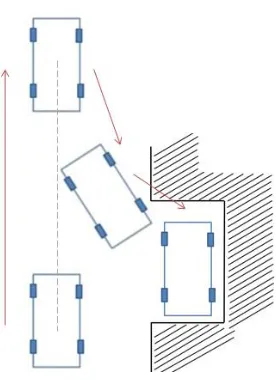
parking process is shown in Figure 1. In this figure, the shadows indicate the walls while

the rectangles represent the vehicle. The vehicle firstly drives past the target parking

space and stops. Then, it starts to reverse into that space. Finally, makes some

adjustments to park the vehicle in the prefect position of the parking spot.

Figure 1: The normal parallel parking process.

However, people sometimes have collisions during this parking process.

Especially when the driver is making some adjustments in the parking spot since the

vehicle might be too close to the walls during this process. Therefore, the automatic

parallel parking will definitely help the drivers make the parking process more effective

(16)

4

1.2 Researches on Automatic Parking

There is no doubt that automatic parking system is constantly improving over the

years [5]. We can see that the automakers nowadays have been implementing the

automatic parking technologies on the vehicle to provide a better driving experience for

people and certainly, these automatic parking systems are benefited from previous

researchers' hard working in this field.

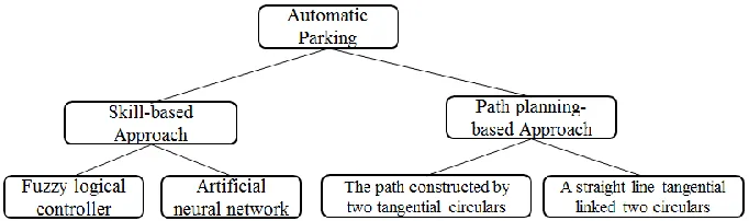
The solutions of automatic parking problem can be generally categorized into two

types: skill-based approaches and path planning-based approaches [6]. The classification

is shown as below:

Figure 2: The classification of automatic parking.

1.2.1 Skill-based Approach

There are two main branches in skill-based parking approaches: fuzzy logical

controller and artificial neural network [6].

In [7], the authors presented a skill-based approach. The idea is about a three-step

(17)

5

the parking space with the vehicle in a ready-to-reverse position. Then, the vehicle is

reversed into the maneuvering space. Lastly, move forward to adjust the vehicle’s

position inside the parking space. The authors indicated that the fuzzy logic techniques

can be applied to each step in the technique outlined.

The authors simulated the parking process with the ATRV-Jr Robot five times

and also observed the robustness during the parking process. The analysis conducted

indicated that the developed algorithm has the ability to parallel parking the robot into a

parking spot that is 1.4 times of the length of the vehicle.

In [6], the authors proposed an algorithm based on a fuzzy logic controller, using

the vehicle pose for the input and the steering rate as the output. A vision sensor and

ultrasonic sensors are used to localize the vehicle. The algorithm automatically learns an

optimal fuzzy if-then rule set from training data. Fuzzy logic controller parameter

optimization can be achieved using a genetic fuzzy system.

The experiment of this algorithm points out that the authors have improved the

current system so that parking from any position can be done with relative ease.

The third approach is brought from [8]. The presented parking processes are as

follows: First of all, the vehicle model is established, and then the parking trajectory is

planned into four stages based on the vehicle model: in the first stage, the vehicle adjusts

(18)

6

system processor calculates the tangency point. Next, the vehicle starts to reverse by

turning the wheels to the right. In the last stage, the vehicle adjusts to find the target

parking point. Meanwhile, the constraints for parking are calculated. Fuzzy control

algorithm is used to track the vehicle parking movement.

The authors stated that compared with previous methods, shorter response time is

observed.

The last skill-based approach is proposed in [9]. The new method in this paper is

described as follows: the segmentation of the parking path is performed to have an

entering segment and a back-and-forth shuttling segment. The entering segment is based

on the two-steps method, which guide the vehicle into the parking spot. The shuttling

segment uses the circular arc of minimum radius of the vehicle to adjust the path until an

optimal target position is found.

Multiple types of curves are taken into consideration and multiple solutions are

presented. A performance measurement matrix, which includes moving distance, control

efforts and path smoothness, etc., is implemented to select the ideal path solution. In the

real application setting, the controller presents multiple paths and the driver is asked to

(19)

7

The experiment was implemented successfully and the result shows that a feasible

path with any starting position based on driver’s select mode can be successfully planned

using segmental path planning technique.

1.2.2 Path Planning-based Approach

Compared with the skill-based approach, path planning-based approach is easier

to understand since it meets people’s driving habits. It is worth emphasizing that the size

of the parking space has a great impact on parking complexity, however, this has not been

discussed sufficiently in most of the previous research papers. Though some of them have

mentioned the smallest space, there are still rooms for improvement.

In [10], the authors proposed a path planning-based algorithm. It plans the parking

path by two tangential circles. The process is divided into four steps. In the first step, the

vehicle moves to the assigned starting point from the initial position. Then, the vehicle

moves to the tangential point of the two circles. And at the third step, the driver changes

the direction of the vehicle, which is the opposite direction of the steps above. Finally,

some adjustments are taken in order to park the vehicle in the target position of the

parking spot.

After the simulation, the authors pointed out that the result shows that the path

planning-based method proposed in this paper has achieved not only parking the vehicle

(20)

8

parking space. The selections of the starting point are more flexible and make the whole

parking process more convenient.

The authors in [11] proposed two improved path planning-based approaches:

geometrically minimum radius path planning-based approach and unequal radius path

planning-based approach. Because the path from the starting point to the destination point

are two arcs from two circles, so obviously unequal radius path planning-based approach

means that two circles have different sizes, it is effective in the situation where the

starting point is far away from the parking spot. The minimum radius path

planning-based approach means that the two arcs are from two circles of the same size, this is

effective in the situation where the parking spot is tighter and the starting point is close to

the parking spot.

The authors simulated both approaches and the result shows that the entire

parking process can be optimized using the combination of the two algorithms. Also, the

scope of the application can be significantly increased.

A new method which improved the approach of fifth-order polynomial is

presented in [12]. Penalty function and genetic algorithm are used for calculations. In

order to minimize the steering angle at the destination position, with parking boundaries

in consideration, an ideal starting position and the fifth order polynomial path curve is

(21)

9

The simulation was based on a real Toyota Camry Sedan 2008 with the following

dimensions as Table 1 shows and we will use the same dataset for comparison in the

simulation chapter.

Table 1: Dataset of the experiment vehicle in paper [12].

The simulation successfully presented the result of parking path without any

collision and the analysis indicated that smaller parking space and shorter parking time

can both be achieved with this method.

In the end, the authors stated that comparing with the other four reference papers

as Table 2 shows, the requirement of the length of parking spot is the smallest among all

five methods. The details of this comparison will be further discussed in the simulation

chapter.

Table 2: Smallest constraint space in different researches [12].

In [14], a new approach was proposed: the car is equipped with ultrasonic sensors

and cameras that gather environment mapping information constantly while driving. The

Name of the argument Data

Length of the vehicle 4.825m

Width of the vehicle 1.82m

Length from front wheel axle to rare wheel axle

2.755m

The Maximum Steering Angle 45˚

Paper [12] [10] [7] [16] [17]

(22)

10

system will be searching for suitable parking spots with the smallest space requirements

in consideration. Once the spot is found, the system generates parking path using the

maximum turning angle with collision avoidance taken into consideration. Then the

motor system controls the car to follow the path and stops vehicle after driver’s

confirmation.

The authors pointed out using simulation that the proposed algorithm is able to

produce smooth parking path that satisfies different parking requirements.

1.3 Contributions

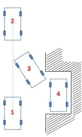
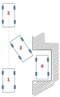
As we have mentioned before, the normal parallel parking process is taken as

what has been shown in Figure 3. In this figure, the shadows indicate the walls while the

rectangles represent the vehicle. The numbers on the center of the vehicle represent the

position number of the parking process. The drivers start at position 1, then, pass the

potential parking spot and stop at the position 2. From positon 2 to position 4, the

skill-based approaches or path planning-skill-based approach are usually used as we have just

(23)

11

Figure 3: Parallel parking process.

In this paper, we propose a method that improves the parking process from

position 3 to position 4. As we mentioned before, people sometimes have the collision

during the process from position 3 to position 4 since the vehicle is getting closer to the

obstacles during this process. The proposed approach will not only help the driver park

safely during this process but also will decrease the required length of the spaces for

parking spots. More spaces will be saved so that the cities could be able to meet the

increasing demand of the parking space in the urban areas.

The proposed method also could be combined with skill-based approach or path

planning-based approach. Most parking process of skill-based approach and path

planning-based approach in previous researches are “one-step” parking. They start to

adjust their path from position 2 and there is no more adjustment when the vehicle is on

(24)

12

approach or path planning-based approach is just used from position 2 to position 3, and

from position 3 to position 4, the proposed method will be used.

Even though the proposed method is not a “one-step” parking solution, however,

it could potentially park vehicles into tight parking spaces which previously proposed

methods may fail to do so.

The rest of the paper is structured as follows. The carefully explained idea and the

details of the approach will be introduced in Chapter two and three, the simulation using

java GUI and Lego EV3 will be presented n Chapter four. The conclusion is in Chapter

(25)

13

Chapter 2 Methodology

In this chapter, the details of proposed approach will be presented. Sections 2.1

and 2.3 will introduce some previous research results that will be used in the proposed

approach. Section 2.2 and 2.4 will introduce the main idea of the proposed approach.

2.1 The Trajectory of Vehicle

In order to study the automatic parking system, we need to study the trajectory of

the vehicles first. A well-constructed vehicle model will allow us to study the trajectory

better. In [11], the authors introduced a vehicle model in Figure.4 to help illustrate the

movement of the vehicle.

(26)

14

In this figure, the center of front wheel axle is represented as (xf, yf ) while the

center of rear wheel axle is represented as (xr, yr). And, l represents the length from the

front wheel axle to the rear wheel axle, w represents the width of the car, δ represent the

steering angle, and the μ represents the orientation of the car.

The following equation is derived in [11] as the trajectory of the center of rear

wheel axle:

( xr-a)2 + (yr – b)2 = (l ⋅ cot δ)2,

where {𝑎 = 𝑥𝑟0− 𝑙 ⋅ 𝑐𝑜𝑡𝛿 ⋅ 𝑠𝑖𝑛𝜇0

𝑏 = 𝑦_𝑟0− 𝑙 ⋅ 𝑐𝑜𝑡𝛿 ⋅ 𝑐𝑜𝑠𝜇₀ , and (xr0, yr0, μ0) represents the initial value of (xr, yr,

μ).The initial value is the value when the vehicle is at its initial position in the coordinate

system.

It was shown in [11] that the trajectory of (xr, yr) is a standard circle from

equation (1). Similarly, if the vehicle is moving with a certain steering angle, the

trajectory of any point on the vehicle could be considered as a finite arc. Moreover, when

the vehicle is moving, the trajectory circles of all four wheels form four circles that share

the same center as shown in Figure 5.

In Figure 5, we can see the four wheels share the same center of circle. Rz is the

length from the center of the rear wheel axle to the center of the circle.

(27)

15

Figure 5: Four wheels share the same origin [11].

2.2 The Coordinate System

After we learned the trajectory of the vehicle, we build our coordinate system for

the proposed approach.

(28)

16

As Figure 6 shows, the blue rectangle represents the vehicle. The coordinate of

the top-right of the vehicle is (xca, yca), and the coordinate of the right,

bottom-right and top-left are respectively (xcb, ycb), (xcc, ycc) and (xcd, ycd). Similarly, the

coordinate of the top-right of the parking spot is (xpa, ypa), and the coordinate of the

bottom-right, bottom-left and top-left are correspondingly (xpb, ypb), (xpc, ypc) and (xpd, ypd).

And, z represents the center of rear wheel axle, w represents the width of the vehicle

while l represents the length of the vehicle. Also, lz represents the length from rear wheel

axle to the back of the car. Rzis the radius of the circle when the front wheels pose at their

maximum steering angles. Oc is the origin of the coordinate, which is never changed

during the whole calculation and the distance between Oc and the center of rear wheel

axle z is Rz. Additionally, the line connecting Oc and z is parallel to the line connecting

(xpb, ypb) and (xpc, ypc).

(29)

17

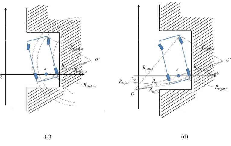
(c) (d)

Figure 7: The coordinate system used in proposed approach while the vehicle is moving.

We further explain the use of this coordinate system in four different diagrams in

Figure. 7. While the vehicle is moving, the (xca, yca), (xcb, ycb),(xcc, ycc) and (xcd, ycd) still

represent the four corner points of the vehicle while the (xpa, ypa), (xpb, ypb),(xpc, ypc) and

(xpd, ypd) represent the four corner points of the parking spot as shown in Figure 7 (a), and

Oc still represents the origin of coordinate.

When the vehicle is moving, we call the circular trajectory of the forward moving

vehicle as moving-forward circle as the dotted arc shows in Figure7 (b) and similarly call

the circular trajectory of the backward moving vehicle as moving-backward circle as the

dotted arc shows in Figure7 (c). In Figure7 (b), Rleft-a, Rleft-b and Rleft-c represent the

(30)

18

Figure7 (c), Rright-a, Rright-b and Rright-c represent the radius of the trajectory of the

top-right, bottom-right and the bottom-left of the vehicle.

As we can see in Figure 7 (d), it shows the relationship between O and O’. O is

the center of the moving-forward circle and O’ is the symmetric point of the O, which is

also the center of the moving-backward circle. Moreover, the knowledge from the path

planning-based approaches is also used here [11]. As Figure 7 (d) shows, the center of

rear wheel axle z is the tangential point to the two trajectory circle connect the

moving-forward circle and moving-backward circle. So O and O’ are symmetric points and z is

their center point.

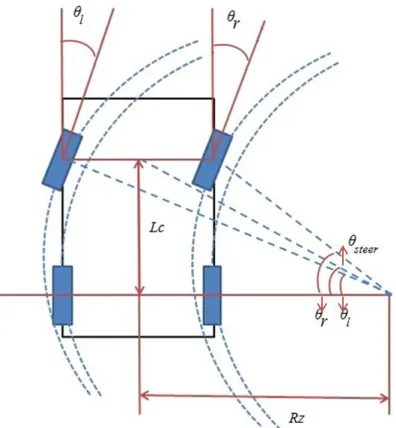
2.3 The Maximum Steering Angle

The maximum steering angle is an important parameter that will be used in the

proposed approach.

The maximum steering angle 𝜃_{𝑠𝑡𝑒𝑒𝑟} is shown in Figure 8. As we mentioned before,

the trajectory circles of all four wheels form four circles that share the same center of the

circle. And the angle between the line connecting this center to the center of the front

wheel axle and the line connecting this center to the center of the rear wheel axle, is the

maximum steering angle 𝜃𝑠𝑡𝑒𝑒𝑟. Once the data of the vehicle is obtained, the maximum

(31)

19

geometrical relationship between the maximum steering angle 𝜃𝑠𝑡𝑒𝑒𝑟 and the minimum

turning radius Rz is shown in Figure 8.

Figure 8: Geometrical relationship between the maximum

steering angle and the minimum turning radius [13].

In Figure 8, 𝜃_𝑙 and 𝜃_𝑟 are the steering angle of the left front wheel and the right

front wheel respectively. The 𝜃_{𝑠𝑡𝑒𝑒𝑟} is the maximum steering angle, which can be

calculated by using 𝜃𝑙 and 𝜃𝑟. And also, the relationship between the maximum steering

angle 𝜃_{𝑠𝑡𝑒𝑒𝑟}and the minimum turning radius Rz can be found. In [13], the authors show

(32)

20

In the proposed method, the maximum steering angle will determine the most

appropriate turning angle of each movement.

2.4 The Proposed Approach

As we mentioned in Chapter 1 or 2, an approach that improves the parking

process from position 3 to position 4 is proposed in this thesis. The parking process in the

proposed approach is shown as below:

1) The proposed approach firstly requires the length and width information of the

vehicle, and also need to know the length and width information of the parking

spot by sensor.

2) Next, it has to determine the target position of the vehicle in the parking spot, as

position 4 in Figure 9.

3) Then, the algorithm using the target position (position 4) as the starting point to

calculate and determine if it is possible to move out from the parking spot

successfully without any collision, and memorize the steps from position 4 to

position 3.

(33)

21

4) Finally, combine with the skilled-based approach [6-9] or path planning-based

approach [10-14] to move the vehicle from position 2 to positon 3 and reverse the

process from position 4 to position 3.

The key process of the proposed approach is to develop an algorithm that is used

for the movement from position 4 to position 3, which will be presented in the following

sections.

Figure 9: Parallel parking process.

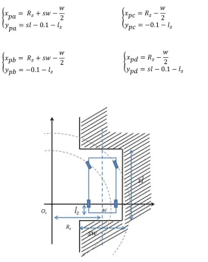
The target position of the vehicle in the parking spot (as position 4 in the figure)

has to be determined first. Sensor gets the information of the length of the parking spot,

which is denoted as sl and the width of the parking spot, which is denoted as sw.

The coordinator of four corner points of the parking spot is shown as in equation

(34)

22

10 and are introduced in the previous section. The coordinates (xpa, ypa), (xpb, ypb), (xpc, ypc)

and (xpd, ypd) are still the parameters of the parking spot. The safe distance is set as 0.1m

in the equation in our proposed method. However, it can be changed base on the real

situation. , We have equation (3) as below given of the geometric relationship between

the vehicle and the parking spot.

Figure 10: The parameter settings in equation (3). {𝑥𝑝𝑏 = 𝑅𝑧+ 𝑠𝑤 −

𝑤 2 𝑦𝑝𝑏 = −0.1 − 𝑙𝑧

{𝑥𝑝𝑎 = 𝑅𝑧+ 𝑠𝑤 − 𝑤 2 𝑦𝑝𝑎 = 𝑠𝑙 − 0.1 − 𝑙𝑧

{𝑥𝑝𝑐 = 𝑅𝑧− 𝑤

2 𝑦𝑝𝑐 = −0.1 − 𝑙𝑧

{𝑥𝑝𝑑 = 𝑅𝑧− 𝑤 2 𝑦𝑝𝑑 = 𝑠𝑙 − 0.1 − 𝑙𝑧

(35)

23

After the length and width of the parking spot are known as well as the target

position and data of the vehicle are known, the algorithm starts to calculate the possible

vehicle movement for parking from position 4 to position 3. The algorithm will be

divided into two parts: when the vehicle going forward and when the vehicle going

backward. As it has been mentioned in the sections above, the trajectory of vehicle is a

standard circle, so the center of the circle is changing while the direction of the vehicle is

changing. The center of moving-backward circle O’ is the symmetric point of the center

of moving-forward circle O, and they are symmetric with the center of rear wheel axle z.

The detail of the calculation of O, O’ and z will be introduced in chapter three.

When the vehicle is moving forward as Figure 11 shows, we set the top-right

point of the vehicle as the tracking point, the coordinate of this point is (xca, yca).

Figure 11: The arc of left turn and the tracking point (xca, yca).

(xca,yca)

Oc

l

lz w

(36)

24

In Figure 11, the vehicle is turning left, which indicates that the top-right point of

the vehicle is moving to the left side of Figure 11, xca is continuously decreasing while

the vehicle is moving forward.. In the meantime, the yca starts to increase its value since

the vehicle is moving forward. The geometrical relationship restricts e xca and yca on the

path of the trajectory circle, which has the coordinate Ocas the origin and the Rz as the

radius. Also consider avoiding the collision in the parking spot, the corners of the vehicle

should not hit the wall or other obstacles, so the value of yca should be less than ypa.

Similarly the value of xcb should be less thanxpb, the value of ycc should be less than ypc.

All these constraints can be summarized in Equation (4) below. In this equation, x0and y0

are the initial value of xca and yca, the initial value is the value when the vehicle is parked

at the target position.

yca = Max ( 𝑦𝑜+ √(𝑙 − 𝑙𝑧)2+ (𝑅𝑧+ 𝑤 2)

2

− (𝑥𝑐𝑎− 𝑥0)2 )

where xca 𝜖 [x'ca, xpd].

Figure 12: The arc of right turn and the tracking point (xcb, ycb). yca<ypa,, xcb<xpb,, ycc>ypc

(4)

Oc (xcb,ycb)

l

(37)

25

Similarly, when the vehicle is moving backward as Figure 12 shows, we set the

bottom-right point of the vehicle as the tracking point, the coordinate of this point is (xcb,

ycb).

The tracking point xcb firstly increases since the vehicle is moving backward, in

this situation, the bottom-right point of the vehicle is moving to the right side of Figure

12. In the meantime, ycb starts to decrease its value since the vehicle is moving backward.

And the geometrical relationship restricts xcb and ycb on the path of the trajectory circle,

Rzis still the radius but the origin is totally different this time. Also considering avoiding

collision in the parking spot, the corners of the vehicle should not hit the wall, so the

value of yca should be less than ypa. Similarly, the value of xcb should be less thanxpb, the

value of ycc should be less than ypc. All these constraints can be summarized in Equation

(5) below, in which x0and y0 are the initial value of xcb and ycb, andthe initial value is the

value when the vehicle is parked at the target position.

ycb = Max ( y0 −√𝑙𝑧2+ (𝑅𝑧−

𝑤 2)

2

− (𝑥0− 𝑥𝑐𝑏)2) )

where xcb ϵ [x'cb, xpb].

Once the coordinate of the (xca, yca) and (xcb, ycb) are known, the localization of

the other three points of the vehicle are still needed, since the position of the vehicle has

to be tracked. This will be introduced in Chapter 3.

(38)

26

Chapter 3 Kinematics Model

In this chapter, a brief introduction of robot kinematics model will be presented.

Implementing the robot kinematics on the proposed vehicle model could help us track the

vehicle during its movement.

Also, by using the geometric solution of robot forward kinematic, the parking

process can be calculated without heavily relying on sensors.

3.1 Robot Kinematics

The main focus of the study of robot kinematics is the motion of bodies but

without considering the forces or moments that result from the motion itself [15]. Robot

manipulator behaviours require sophisticated robot kinematics modeling in order to be

properly analyzed. Thus, formulating the appropriate kinematics models for suitable

robot mechanism is very important in studying and analyzing the motion of robot

manipulator, which is commonly known as robot kinematics [15].

There are two types of robot kinematics, forward kinematics and inverse

(39)

27

Figure 13 will help us explain these two types of robot kinematics more clearly. In

this figure, there is a two-link arm kinematic model. In this figure, l1 and l2 represent the

links, θ1 and θ2 represent the angles of joints.

Figure 13. Two-link arm kinematic model [15].

We can explain the two kinds of robotic kinematics briefly below [15]:

• Forward Kinematics is used when the length of each link and the angle of each

joint is known, and can be used to calculate the position of any point.

• Inverse Kinematics is used when the length of each link and the position of some

points on the robot is known, and can be used to calculate the angles of each joint needed

to obtain that position.

In this thesis we will use forward kinematics which is also called direct

(40)

28

3.1.1 Implement the Forward Kinematics on the Vehicle Model

In the proposed approach, a 2-dimensional arm’s forward kinematic model is used.

The using of forward kinematic model allows us to be able to calculate the coordinate of

the corner points of the vehicle by using some links and the angles of joints.

As we can see in Figure 14, we implement the forward kinematic model on our

vehicle model.

Figure 14: Kinematic model implement on the proposed vehicle model.

We set the line that connecting the origin Oc of the coordinate system and the

centerof moving-backward circle, which is O’,as the first link l1 in the kinematic model.

And, respectively, the second link l2 is the line connecting O’, the center of

moving-backward circle, and the bottom-right point of the vehicle. The second link may also be

top-right of the vehicle since it depends on whether the vehicle is moving forward or

moving backward as we mentioned in chapter two. Angle θ1 is the angle between the l1

and the x- axis while the 𝜃2 is the angle between l1’s extended line and l2 in anticlockwise.

Oc

(41)

29

From [15], the authors presented the figure 15, where l1, l2 are the links, θ1 and θ2

are the angles of the joints, and p is a point that could be calculated by using forward

kinematic.

(a) (b)

Figure 15: Two-arm Kinematic model [15].

Figure 15 (a) presents a manipulator, and its spatial geometry can be broken down

into smaller geometry problems as shown in Figure 15 (b).

As we can easily see in Figure 15 (b), we have the following equation (6):

Px = l1 ∙ cos 𝜃1 + l2 ∙ cos 𝜃12

Py = l1 ∙ sin 𝜃1 + l2 ∙ cos 𝜃12,

where 𝑐𝑜𝑠𝜃12 =𝑐𝑜𝑠𝜃1 ∙ 𝑐𝑜𝑠𝜃2 − sin 𝜃1∙ sin 𝜃2 , and 𝑠𝑖𝑛𝜃12 =𝑠𝑖𝑛𝜃1 ∙ 𝑐𝑜𝑠𝜃2+cos 𝜃1∙ sin 𝜃2 ,

and 𝑐𝑜𝑠𝜃12 denotes cos (𝜃1+ 𝜃2).

In [15], it was demonstrated that 𝜃2 can be derived as below:

(42)

30 𝜃2 =Arc tan ( ±

√1−(𝑝𝑥2+𝑝𝑦2−𝑙12− 𝑙2 2

2𝑙1𝑙2)

𝑝𝑥2+𝑝𝑦2−𝑙12− 𝑙2 2

2𝑙1𝑙2 )

However, there are two possible values for 𝜃₂ and it is not easy to rule out any

one of them since the difference of the two results are small, it has to use some other

restrictions to find the right one, which make the calculation process even more complex.

Therefore, we introduce the notion of intersection angle to solve this problem.

3.2 The Intersection Angle

The intersection angle is the angle between the line connecting O’, the center of

the moving-backward circle and the tracking point, and the line connecting O’ and any

corner points on the vehicle. The intersection angle helps us to know the angle of the joint

instead of finding the right 𝜃₂ in two possible 𝜃₂ from equation (7).

Here we are using (xcc, ycc) as an example. We are looking for the coordinate of

the bottom-left point of the vehicle which is (xcc, ycc). The intersection angle δ is the angle

that between the line connecting O’ and the point (xcb, ycb) and the line connecting O’ and

(xcc, ycc). 𝜃2 is the angle between the l1’s extended line and the l2 in anticlockwise while θ3

is the angle between the l1’s extended line and the l3 in anticlockwise. l3 is the link

connect the O’ and (xcc, ycc). In this figure, l is still the length from the head of the vehicle

to the rear wheel axle while the lzis the length from the rear wheel axle to the end of the

vehicle. W is the width of the vehicle and z is still the center of the rear wheel axle.

(43)

31

Figure 16: The intersection Angle.

Here we use (xcb, ycb) as the tracking point, so the coordinate of it is known as we

introduced in Chapter 2. Then, because l1, l2 and 𝑐𝑜𝑠 𝜃1 are also known, by using

equation (6), the cos𝜃₁₂ could be deduced. And for (xcc, ycc), the angle of the joint is the

difference between 𝜃₁₂ and 𝛿 as shown in Figure 16.

Therefore, we have the following equation 𝑐𝑜𝑠𝜃₁₂ = 𝑐𝑜𝑠𝜃₁ ∙ 𝑐𝑜𝑠𝜃₂−

𝑠𝑖𝑛 𝜃1∙ 𝑠𝑖𝑛 𝜃2 and 𝑠𝑖𝑛𝜃12 = 𝑠𝑖𝑛𝜃1∙ 𝑐𝑜𝑠𝜃2+ 𝑐𝑜𝑠 𝜃1∙ 𝑠𝑖𝑛 𝜃2 are equivalent to the

equation (8) by using the intersection angle:

𝑐𝑜𝑠𝜃_12𝛿 = 𝑐𝑜𝑠𝜃₁₂ ∙ 𝑐𝑜𝑠𝛿 − 𝑠𝑖𝑛 𝜃₁₂∙ 𝑠𝑖𝑛𝛿

𝑠𝑖𝑛𝜃_12𝛿 = 𝑠𝑖𝑛𝜃₁₂ ∙ 𝑐𝑜𝑠𝛿 + 𝑐𝑜𝑠𝜃₁₂∙ 𝑠𝑖𝑛𝛿.

(8) Oc

l2

(44)

32

3.3 The Update of the Center of Circle

As we mentioned in chapter two, since the vehicle is moving, the center of the

rear wheel axle z also has been changed. Besides, when the vehicle changes its turning

direction, the center of the trajectory circle is changed as well, thus, the update of the

center of the trajectory circle is required.

The new z is required to be calculated at first. Since the bottom-right point (xca,

yca) of the vehicle is known when it is the tracking point, so we use the relationship

between this point and z to derive the coordinate of z as explained in Figure 17.

In Figure 17, φ1 is the angle between lz and the line connecting (xcb, ycb) to z, φ2 is

the angle between the line connecting top-right corner and bottom-right corner, and

x-axis. Since (xca, yca) and (xcb, ycb) are known as we discussed in chapter two, the distance

between (xcb, ycb) and z are fixed, so we could derive that φ1=arc tan

𝑤/2

𝑙𝑧 , φ2=arc tan

𝑦𝑐𝑎−𝑦𝑐𝑏

(45)

33

Figure 17: The symmetric origin of the circle.

Lz is still the length from the rear wheel axle to the back of the vehicle while the w

is the width of the vehicle. ∆𝑥and ∆𝑦 are the change of the coordinate of z on x-axis and

y-axisrespectively. Then we have equation (9):

∆𝑥 = 𝑐𝑜𝑠𝜀 ∙ √𝑙𝑧2+ (

𝑤 2)

2

𝑥𝑧=xcb- ∆𝑥;

∆𝑦 = 𝑠𝑖𝑛𝜀 ∙ √𝑙𝑧2+ (

𝑤 2)

2

𝑦𝑧=ycb- ∆𝑦;

After z is updated by equation (9) above, O’, the center of the moving-backward

circle is not difficult to be calculated based on the information of O, the center of the

moving-forward circle and z.

(46)

34

3.4 The Final Equation

So, combine the equations (4) to (9) that we derived in the previous two chapters,

we have the final equation as equation (10) to equation (12) shown:

(10)

(11)

(47)

35

Chapter 4 Implement and Experiment Result

In this chapter, the simulation using JAVA GUI and experiment with Lego EV3

will be presented. The details of the simulation are presented in section 4.1, which

includes the programming environment, the introduction of dataset, and the results. The

details of the experiment with Lego EV3 are presented in section 4.2, which includes the

introduction of the Lego EV3 robot, the calibration before the experiment, and the results.

4.1 The Simulation using JAVA GUI

In this section, the details of the simulation using JAVA GUI of the proposed

method are discussed. The result shows that the proposed method successfully saves up

to 17% of the required spaces of parking spots compared to previous research.

4.1.1 The Simulation Setup

We use JAVA for programming and use JAVA GUI to draw the position of each

movement of the vehicle in this experiment. The IDE we use for Java is Eclipse Kepler

(48)

36

The standard of comparisons we use is Smallest Constraint Space (SCS). It is

used in many other previous researches; we also use it here so that our result could be

comparable with others’ results. From [12], SCS is defined as：

Smallest Constraint Space (SCS) =length of parking spot

length of the vehicle .

As we can see from the definition, the smaller of the SCS value, the less spaces of

the parking spot is required.

The data we used in simulation is based on Toyota Camry Sedan 2008 model with

the following dimensions: the length is 4.825 m, width is 1.82 m, and the length from the

front wheel axle to the rare wheel axle is 2.755 m. The maximum steering angle is 45

degree. Our simulation follows the proportion of the Toyota vehicle and scales

proportionally so that the result could fit screen. However, the author in [12] did not

mention the safe distance, and in our simulation we used 0.1m as our safe distance here

as we have mentioned before in Chapter two, equation (3).

Figure 18 shows a straight forward picture about the vehicle we simulate. It is the

same vehicle model from [12] since we will compare it with our proposed approach. In

Figure 18, l1 is the length from the head of the vehicle to the front wheel axle, l is the

length from the front wheel axle to the rear wheel axle. Similarly l2 is the length from the

(49)

37

Figure 18: The dataset of the vehicle for simulation [12].

4.1.2 The Simulation Process and Result

Table 3 shows the required input information for simulation and the outputs of the

simulation program.

Input Information Output of the simulation

 Length sl and width sw of the parking spot

 Length from rear wheel axle to the back of

the car lz

 Maximum steering angle θsteer

 Length l and width w of the vehicle

 Length of the safe distance

 Length of the smallest parking spot

 The GUI result

 The coordinate of four corner

points of the vehicle during the

parking process

Table 3: The input and output of the simulation program.

We input the data into the program, the results indicate that the smallest parking

(50)

38

The result is shown in Figure 19. The red rectangles represent the vehicle while

the black lines represent the wall or any objects that the vehicle cannot hit. The number at

the top-right corner of the rectangles are counters, we set each red rectangle in the figure

represent a ‘movement’ of the vehicle, so as we can see there are 10 movements of the

parking process in Figure 19. The counter number 0 means the final stopped position of

the vehicle and number 10 is the starting point of the automatic parallel parking.

Figure 19: The movements in a parking process.

Table 4 shows the coordinate of four corner points of the vehicle during the

parking process. The number on the left column is the number of each movement as

(51)

39

Table 4: The tracking data of each movement during a parking process.

Table 5 shows the Smallest Constraint Space of other researchers’ methods [12].

As we can see from Table 5, the best SCS of previous researches is 1.35. The approach

that is proposed in [12] used the same Toyota model and it requires 6.51375 meters for

the length of parking spot while the proposed approach in this thesis just requires 5.3674

meters.

Table 5: Smallest constraint space in different researches.

Table 6 shows the comparison of the approach from [12] and the proposed

approach. As it is shown in Table 6, the proposed approach has improved the possibility

to park into a tight parking spot from SCS 1.350 to SCS 1.113. When the SCS is smaller

than 1.110, both of the approaches could not park the vehicle in the parking spot. As we Counter

0 (Xca, Yca)=(4, 3) (Xcb, Ycb)=(4, -1) (Xcc, Ycc)=(2, -1) (Xcd, Ycd)=(2, 3)

1 (Xca, Yca)=(3.7, 3.363034) (Xcb, Ycb)=(4.076342, -0.61922) (Xcc, Ycc)=(2.085214, -0.80739) (Xcd, Ycd)=(1.708872, 3.174863) 2 (Xca, Yca)=(3.484931, 3.173651) (Xcb, Ycb)=(4.176342, -0.76614) (Xcc, Ycc)=(2.206447, -1.11185) (Xcd, Ycd)=(1.515036, 2.827945) 3 (Xca, Yca)=(3.184931, 3.433534) (Xcb, Ycb)=(4.186667, 0.439) (Xcc, Ycc)=(2.2504, -0.93987) (Xcd, Ycd)=(1.248664, 2.932666) 4 (Xca, Yca)=(3.033046, 3.252048) (Xcb, Ycb)=(4.286667, -0.54643) (Xcc, Ycc)=(2.387428, -1.17324) (Xcd, Ycd)=(1.133807, 2.625237) 5 (Xca, Yca)=(2.733046, 3.445531) (Xcb, Ycb)=(4.254496, -0.25382) (Xcc, Ycc)=(2.404822, -1.01454) (Xcd, Ycd)=(0.883371, 2.684806) 6 (Xca, Yca)=(2.621526, 3.269091) (Xcb, Ycb)=(4.354496, -0.33602) (Xcc, Ycc)=(2.551942, -1.2025) (Xcd, Ycd)=(0.818971, 2.402606) 7 (Xca, Yca)=(2.321526, 3.412512) (Xcb, Ycb)=(4.290286, -0.06944) (Xcc, Ycc)=(2.54931, -1.05382) (Xcd, Ycd)=(0.58055, 2.428132) 8 (Xca, Yca)=(2.239861, 3.239804) (Xcb, Ycb)=(4.390286, -0.13298) (Xcc, Ycc)=(2.703894, -1.20819) (Xcd, Ycd)=(0.553469, 2.164591) 9 (Xca, Yca)=(1.539861, 3.446147) (Xcb, Ycb)=(4.158345, 0.422318) (Xcc, Ycc)=(2.646431, -0.88692) (Xcd, Ycd)=(0.027946, 2.136905) 10 (Xca, Yca)=(1.439367, 2.946085) (Xcb, Ycb)=(4.458345, 0.3221) (Xcc, Ycc)=(3.146307, -1.18748) (Xcd, Ycd)=(0.127329, 1.436596)

Coordinate

Paper [12] [10] [7] [16] [17]

(52)

40

have mentioned before, the proposed method is not a “one-step” method but it does

enable to park the vehicle into a narrower space.

SCS Length of parking spot

(meter) [12]

Number of

steps Approach Proposed Number of steps

1.350 6.51375 √ One-Step √ One Step

1.300 6.27250 × N/A √ One Steps

1.280 6.17600 × N/A √ One Steps

1.250 6.03125 × N/A √ Three Steps

1.200 5.79000 × N/A √ Three Steps

1.180 5.69350 × N/A √ Four Steps

1.150 5.54875 × N/A √ Four Steps

1.113 5.37022 × N/A √ Ten Steps

1.110 5.35575 × N/A × N/A

Table 6: Comparison with previous research result.

Compared with the new approach that this paper proposed, the proposed method

potentially saves up to 1.350−1.113

1.350

=

17.6% of the parking space.

Table 7 shows the different parking processes from SCS 1.300 up to 1.113.

As we can see, when the SCS is 1.3, the space of parking spot is spacious as well

as when the SCS is 1.28, the vehicle could park into the spot without any stops. Then, the

SCS 1.25 and SCS 1.2 require the vehicle makes some movements for park in the spot.

As the parking spot is becoming tighter, SCS 1.18 and SCS 1.15 requires more

movements to finish the process. Last but not least, as we can see when the SCS is 1.113,

(53)

41 (a)

(b)

Table 7: Different parking process from SCS 1.300 to 1.113.

4.2 The Experiment with Lego EV3

In this section, the detail of the experiment with Lego EV3 is presented. Some

(54)

42

deviations of the hardware and experimental environment. Even so, the experimental

results show that the proposed approach appears to work as expected.

4.2.1 The Experiment Setup

Lego EV3 is the new member of Lego MINDSTORMS series. After the success

of its second generation Lego MINDSTORMS NXT 2.0 robot, the Lego company has

launched its third generation robot Lego EV3 in MINDSTORMS robotics product line

[18].

For the experiment, we use the Lego EV3 robot (EV3) as a model of the real

vehicle and we use the leJOS as the programming language. leJOS is a firmware

replacement for the Lego MINDSTORMS series’ programmable bricks. The Java virtual

machine inside allows Lego EV3 robots to be programmed in JAVA [19].

The IDE we use for Java is Eclipse Kepler with the jre 7u55 and jdk 8u5, and the

leJos firmware is the leJOS_EV3_0.8.1-beta for the EV3.

Figure 20 shows the different sides of the EV3 model vehicle. Figure 20 (a)

shows the chassis of the vehicle, Figure 20 (b) and Figure 20 (c) show the front side and

(55)

43

(a) Chassis (b) Front View

(c) Back View (d) Side View

Figure 20: The different views of the vehicle assembled from Lego EV3.

This vehicle model is finished by using EV3 original package and the expended

package by following the instruction of RAC3 TRUCK on the EV3 official website [20].

This is one of the models that could be used as the real vehicles (4 wheels, rear drive)

(56)

44

The length of the Lego EV3 RAC3 TRUCK is 24cm while the width is 16.5cm.

The length from the front of the vehicle to the front wheel axle is 3cm, and the length

from the front wheel axle to the back of the vehicle is 4cm. We also set the maximum

steering angle as 45 degrees.

4.2.2 The Calibration

Before starting the experiment, the calibration has to be done firstly because there

are some deviations either from the wheels or from the odometer. The performance of

experiment is affected by the condition of the floor, the component of the vehicle model,

the program and other factors.

The first calibration is the turning speed when the EV3 vehicle is moving. Since

the EV3 vehicle constructed is a rear wheel drive type vehicle and during the process of

changing the direction, the front wheels are changing too fast while the rear wheels, in

the meantime, are not stopping moving forward or backward, so there is always a side

slip phenomenon. To calibrate this, we add a stop command to the two motors after each

movement as shown below in the source code.

Motor.A.stop();//A is the name of one of rear motors

(57)

45

The other calibration is, after adding the command above, the motor A and motor

C cannot stop at the same time, which makes the wheels turning more angles than we

expected.

Figure 21: The motors of the EV3.

As we can see in Figure 21, because A and C are the rear wheel motor so if the

motor A stops first and motor C keeps moving, or, motor C stops first and motor A keeps

moving, the motor B and motor D still posit the corresponding wheels in a turning angle,

so the vehicle will still move when it is supposed to stop. In this situation, it will affect

the movements in all the following steps and may lead the vehicle to hit the wall or other

objects. After some research, the modified version of code is shown as below:

Motor.A.stop(true);

Motor.C.stop();

In this two-line code, the motor in the first line will wait a second for the motor in

(58)

46

The finally calibration is the wheels. Both wheels have around a10 degree angle

to the left under natural conditions, thus an extra 10 degrees to the right were added and

calculated in the program.

4.2.3 The Experiment Process and Result

The program we used here are the same as in the simulation part. But the outputs

of the program are the real movements of the EV3 robot instead of the simulated

movements in the GUI.

The EV3 does not have the same proportional data of the vehicle as the real

Toyota has in last experiment. However, we set up a similar experiment and compare the

results using the smallest constraint space. The experiment data is shown in Table 8.

SCS Length of parking spot (cm)

1.875 45

1.400 33

1.250 30

1.200 28.8

1.113 26.712

Table 8: Smallest constraint space in Lego EV3 data set.

We conducted experiments using the SCS data above. We experiment three times

for each SCS. The experiment is considered to be successful if in two out of three

experiments, the EV3 does not hit the wall and exit the parking spot successfully without

any collisions. Otherwise, it is considered to fail.

(59)

47 SCS Length of parking spot (cm) Proposed

Approach Note

1.875 45 √

1.400 33 √

1.250 30 √

1.200 28.8 × Minor collision

1.113 26.712 × Minor collision

Table 9: Result of parking in different Smallest Constraint spaces using Lego EV3.

As we can see, though the length of the parking spot is becoming tighter, the

proposed approach is still able to finish some parking process. However, we have noticed

that during some of the movements, the EV3 slightly hit the wall.

Here are some photo records of the experiments. All of the photos are captured

from the successful experiments. In the photos, the red lines represent the wall or any

other objects that the vehicles are not allowed to hit. The ruler that on the right side of the

photos indicate the length of the parking spot.

The order of the photos is shown as below:

Movement 1 Movement 2

(60)

48

For SCS is 1.875, which means the length of the parking spot is 45cm. The vehicle

could be parked in the parking spot in just one movement without any collisions as it is

shown below.

(61)

49

When the SCS is 1.4, the length of the parking spot is 33cm. Eight movements

are required to finish the parking as it is shown below. We can see that there is also no

any collision.

(62)

50

(63)

51

For SCS is 1.25, the length of the parking spot is 30cm. Seven steps are

required to finish the parking process as shown in the following photos. We observe that

for some of the movements, the head of the vehicle really close to the wall in this

situation.

(64)

52

(65)

53

When the SCS is 1.2, the length of the parking spot is 28.8cm. The vehicle took

twelve steps to finish the parking process. We have noticed there are some small

collisions happened during the experiment.

(66)

54

(67)

55

(68)

56

For SCS is 1.113, the length of the parking spot is 26.712cm. Also twelve

movements are taken to finish the parking process. We also observed some small

collisions.

(69)

57

(70)

58

Chapter 5 Conclusion

5.1 Summary

In this thesis, we proposed an automatic parallel parking approach which

improves the possibility of parking the vehicle into tight parking spaces. We used the

robot kinematics to build the vehicle model and used geometric relationship to restrict

and track the vehicle’s movement to avoid collisions.

Compared with the other approaches, the proposed approach has some improved

features:

• It is a geometrical approach which needs fewer sensors.

The only information that this approach requires from the sensors, is the length

and width of the parking spot. All the calculations are based on the size of the parking

spot and the size of the vehicle.

• It utilizes parking spaces more effectively.

Compared with previous approaches, this approach could potentially save parking

space up to 17.6%, which means for the same rooms, this approach will be able to park

(71)

59

• It could be combined with both skill-based approach and path planning-based

approach. Thus, the automatic parking will suit more situations.

Though some of the previous researches could make the parking process as a

‘one-step’ parking, but the requirement for spaces is larger. The combination of previous

approach and the proposed approach will help promoting the efficiency of the automatic

parking.

In experiments, compared with previous researches, the proposed method saved

up to 17.6% parking spaces in simulation. When the proposed method is implemented on

the LEGO EV3 robot, we can see it also works well most of the time. However, some

collisions are observed since there are some limitations on the Lego EV3 we used in the

experiment. The proposed approach requires a high level of accuracy when the vehicle is

parking in an extreme tight space, but this requirement is not met on LEGO EV3. Even so,

the experiment demonstrates that the proposed approach appears to be feasible.

5.2 Future Work

There is no doubt that the combination of skill-based approaches or path

planning-based approaches will expand the limitation of the length of parallel parking

spots in the future. What’s more, if the accurate performance could get improved, this

method will help to provide a better experience on the automatic parallel parking for all

(72)

60

area in big cities. Research on how to keep the appropriate safe distance for this approach

(73)

61

Appendix

(74)

An Improved Approach for Automatic Parallel Parking in Narrow Parking Spaces

Scholarship at UWindsor

Scholarship at UWindsor

An Improved Approach for Automatic Parallel Parking in Narrow

An Improved Approach for Automatic Parallel Parking in Narrow

Parking Spaces

Parking Spaces

An Improved Approach for Automatic Parallel Parking

in Narrow Parking Spaces

An Improved Approach for Automatic Parallel Parking

in Narrow Parking Spaces

by

Declaration of Originality

Abstract

Acknowledgements

Dedication

Contents

List of Figures

List of Table

Chapter 1

Introduction

1.1 Background

1.2 Researches on Automatic Parking

1.2.1 Skill-based Approach

1.2.2 Path Planning-based Approach

1.3 Contributions

Chapter 2

Methodology

2.1 The Trajectory of Vehicle

2.2 The Coordinate System

2.3 The Maximum Steering Angle

2.4 The Proposed Approach

Chapter 3

Kinematics Model

3.1 Robot Kinematics

3.1.1 Implement the Forward Kinematics on the Vehicle Model

3.2 The Intersection Angle

3.3 The Update of the Center of Circle

3.4 The Final Equation

Chapter 4

Implement and Experiment Result

4.1 The Simulation using JAVA GUI

4.1.1 The Simulation Setup

4.1.2 The Simulation Process and Result

=

4.2 The Experiment with Lego EV3

4.2.1 The Experiment Setup

4.2.2 The Calibration

4.2.3 The Experiment Process and Result

Chapter 5

Conclusion

5.1 Summary

5.2 Future Work

Appendix