An Evaluation of Linux I/O Scheduler Behavior at the Block I/O Layer

(1)

ABSTRACT

SINHA,SUBHAS KUMAR. An Evaluation of Linux I/O Scheduler Behavior at the Block I/O Layer.(Under the direction of Dr. Vincent Freeh.)

Linux comes with four different I/O schedulers - NOOP, Deadline, An-ticipatory, and Complete Fairness Queuing (CFQ). Each scheduler attempts to reduce overall response time using different algorithms involving ordering and merging of I/O requests. These schedulers tend to behave differently for different types of workloads.

In this study we validate the behavior of the different I/O schedulers at the block I/O layer, present our observations and and give our recomomendation regarding what could be the right scheduler for a particular environment. We have restricted our study to a desktop environment.

(2)

An Evaluation of Linux I/O Scheduler Behavior at the Block I/O Layer

by

Subhas Kumar Sinha

A thesis submitted to the Graduate Faculty of North Carolina State University

in partial fulfillment of the requirements for the Degree of

Master of Science

Computer Science

Raleigh, North Carolina 2008

Approved By:

Dr. Xiaohui Gu Dr. Khaled Harfoush

(3)

BIOGRAPHY

(4)

LIST OF TABLES

Table 3.1 Hard disk configuration . . . 19

Table 3.2 List of software . . . 19

Table 4.1 Response times - Deadline . . . 50

(7)

LIST OF FIGURES

Figure 1.1 Linux Block I/O stack. [1] . . . 1

Figure 2.1 BIO [2] . . . 6

Figure 2.2 layout of a page for data transfer. [1] . . . 10

Figure 2.3 noop scheduler . . . 10

Figure 2.4 Deadline scheduler . . . 11

Figure 2.5 Anticipatory scheduler . . . 17

Figure 2.6 CFQ scheduler . . . 17

Figure 3.1 Test platform disk configuration . . . 27

Figure 3.2 Queue time and queue size . . . 27

Figure 3.3 Queue time and size - closeup . . . 28

Figure 3.4 Request size of dispatched requests . . . 28

Figure 3.5 Initial sector accessed for each request . . . 29

Figure 3.6 Queue time and dispatch time for different schedulers. These were generated for a SCSI device. Similar pat-terns were observer for ATA and IDE . . . 30

Figure 3.7 Sector requests for 2 process sequential read for the NOOP and Deadline schedulers . . . 31

Figure 3.8 Sector requests for 2 process sequential read for the Anticipatory and CFQ schedulers . . . 32

Figure 3.9 Queue time and queue size - four process sequential read . . . 34

Figure 3.10 Sector requests for four process sequential read . . . . 35

Figure 3.11 Queue depth and request times - single process stream-ing write . . . 37

(8)

Figure 3.13 CFQ - i/o pattern of dd + cat . . . 40 Figure 3.14 Deadline - i/o pattern of dd + cat . . . 41 Figure 3.15 Noop - i/o pattern of dd + cat . . . 42 Figure 3.16 i/o pattern of 2 dd processes and 2 cat processes . . . 44 Figure 3.17 Sector requests made by a single find - cat processes . 46

Figure 4.1 Comparison read and write I/O requests . . . 48 Figure 4.2 Deadline overcoming the read starvation of Noop. . . 50 Figure 4.3 Comparing the request queuing of one chunk-read

(find-cat) process and one sequential read((find-cat) process be-tween the Anticipatory and the Deadline scheduler . . 52 Figure 4.4 Single process chunk read . . . 54 Figure 4.5 Two process chunk read . . . 54

(9)

Chapter 1 Introduction

The Linux Block I/O subsystem provides the necessary services required for the communication with block devices like hard disks and DVD ROMS. The block I/O subsystem is made of a stack of software components as shown in Figure 1.1..

Figure 1.1: Linux Block I/O stack. [1]

(10)

The I/O scheduler is responsible for scheduling the dispatch of I/O requests. The block device driver is device dependent and communicates directly with the disk device. And at the bottom of the stack we have the actual disks.

Each I/O request has to move down this I/O stack to get scheduled and dispatched to the disk.

1.1 Overview - I/O schedulers

Our focus of study is the I/O scheduler layer. The primary component in this layer is the I/O scheduler . Its job is to maximize I/O bandwidth to the disk while ensuring fairness in I/O request handling amongst the different processes.

The Linux 2.4 kernel had one I/O scheduler - the elevator Linux scheduler in Linux 2.4 [3]. The current 2.6 kernel has four schedulers - NOOP, Deadline, Anticipatory and Complete Fairness Queuing (CFQ).

The NOOP scheduler is a simple scheduler that does request ordering based on sector number and request merging. The Deadline scheduler works on the principle of a limiting threshold latency for each request. The An-ticipatory scheduler induces a brief wait in anticipation of a synchronous I/O read from the same process. The CFQ scheduler tries to distribute the available bandwidth equally amongst different process threads.

The default scheduler in most of the current Linux distributions is CFQ. All the schedulers come compiled with the kernel and are available by default. A default scheduler can be configured either at boot time or at it can be configured for a specific block device at run time.

1.2 Problem Description

(11)

taken this further by analyzing I/O patterns for different types of loads and hardware (i.e. different types of disks).

The goals of this thesis are to understand Linux I/O behavior, use I/O trace tools to effectively capture I/O traffic with minimal overhead, intuitive represent I/O traffic, evaluate the low level I/O behavior of I/O schedulers, and recommend or confirm existing recommendations regarding the preferred I/O scheduler for different I/O loads.

1.3 Significance

Our work is an extension of previous work done related to performance eval-uation of I/O schedulers [7, 8]. Using I/O and kernel trace tools like blktrace and systemtap [9, 10, 11, 13] we capture accurate low level I/O trace details minimal overhead, minimal coding and no kernel modification. This gives us a better picture of I/O activity than mere timing information and we get a better understanding of I/O scheduler behavior.

By careful analysis of the data generated by these tools we can measure and illustrate features of the I/O subsystem like I/O queue size, the disk queue size, the maximum request size that is handled by the underlying disk device.

The combination of blktrace and blktrace systemtap scripts allow us to capture I/O information associated with specific processes and specific files. This level of tracing is possible even in the case of writes where its the daemon process like pdflush which sends the actual request and not the process that actually initiated the write operation. [13]

(12)

1.4 Thesis Organization

(13)

Chapter 2 Background

2.1 Linux Block I/O layer

As indicated in Chapter 1, the Linux I/O subsystem comprises a stacked set of kernel components.

At the top is the Virtual Filesystem switch (VFS) layer . It provides a single interface to multiple underlying filesystems and allows applications to make I/O calls through a generic API which is independent of the filesystem. VFS also manages the filesystem cache.

Themapping layeris responsible for mapping a file name and file offset to a logical block address and similarly map the extent of the request data into number of blocks. The mapping layer computes this information by making filesystem specific calls to retrieve superblock and inode data.

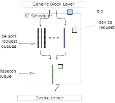
The generic block layer (GBL) converts I/O requests into I/O oper-ations for the lower layers. A I/O operation is represented by a block I/O (BIO) . Each BIO structure, among other things, contains information about the type of I/O (read/write) to perform, device (e.g. disk and partition) on which to perform I/O and information about contiguous blocks to read from /written to. A BIO represents contiguous blocks and hence a single I/O request can result in multiple BIOs

(14)

Figure 2.1: BIO [2]

uses sectors, the buffer cache and the paging system use pages (memory frames). The GBL maps all of this together using bio vec structures. Each BIO consists of a vector of bio vec structures which represents blocks, sectors and memory pages. Figure 2 shows the bio vec’s associated with a single BIO. Figure 3 later shows the relation between the different units of representation. Once the I/O requests get scheduled , the device driver schedules scatter-gather DMA operations with the device controller. The controller does the data transfer of contiguous sectors to the pages in memory pointed to by the bio vec structures. The additional unit here is a segment, which is either a page or part of a page. This is needed by the drivers to facilitate the scatter-gather DMA.

TheI/O scheduler layer inserts I/O request units (BIO) into the I/O queues. This following section provides additional information about the same.

(15)

2.2 Linux I/O Schedulers

The basic unit of data transfer of a block device driver is one sector. The overheads of transferring data one sector at a time are very high and hence the kernel tries to cluster multiple sector requests and issues a single operation to initiate the data transfer.

An I/O read/ write request results in the creation of a block device re-quest. Initially the scheduler creates a block device request and a single BIO is associated with that request. This request is then inserted into the

request queue. The I/O scheduler keeps the requests sorted based on sec-tor numbers. On receiving additional read/ write requests the scheduler will try to do one of the following. In case the new request is for some sectors that are adjacent to sectors associated with an existing queued request, then it extends the queued request. This is done by adding the BIO of the new request to the list of BIO or by extending the existing BIO of the queued request. add the segment to a new BIO. In the case there is no match then the scheduler creates a new request and inserts it into the request queue.

In addition to the request queueeach scheduler maintains a dispatch queue. The request queue is used for the purpose of request ordering and merging while thedispatch queueis a sequence of ordered requests that are ready to be processed. The service routine of the device driver picks up the first request from the dispatch queue and dispatches it to the disk device. There is one queue for each block device driver. In case a device services multiple devices ( e.g. multiple SCSI disks) then there is a queue for each device as well.

(16)

2.2.1 NOOP scheduler

(17)

2.2.2 Deadline scheduler

The deadline scheduler was the first improved scheduler made available after the basic I/O scheduler. It works on the principle that the best way to access a disk is to access in increasing order of sector number. At the same time, to prevent starvation, each request is associated with a deadline by which time it has to be serviced - in the worst case.

Reads have preferences over writes. Read requests are given a deadline of 500 milliseconds and write requests are given a deadline of 5 seconds.

This scheduler has 4 request queues and 1 dispatch queue. There is 1 pair of deadline queues and 1 pair of sorted queues. From each pair one is for read and the other is for write. The sorted queue queues requests in increasing order of sector numbers. The deadline queue is essentially a FIFO queue. Each incoming request is inserted into the sorted queue based on its sector number and added to the tail of the deadline queue along with an associated deadline timer.

The scheduler’s policy for reducing disk seek times is by moving large batches of requests from the sorted lists and then servicing a small number of out of order deadline elapsed requests.

The scheduler uses the following rules (in sequence) to move requests from the request queues to the dispatch queue. Note: write request deadlines are not considered.

If the previous two operations were read request dispatches then the scheduler dispatches a set of write requests and exits.

If there are expired read requests dispatch a set of those requests and exit. If there are requests in the read sort queue dispatch a set of those requests and exit.

If there are write requests in the write sort queue dispatch a set of those requests and exit.

2.2.3 Anticipatory scheduler (AS)

(18)

Figure 2.2: layout of a page for data transfer. [1]

(19)

(20)

queues and 1 dispatch queue . It has smaller deadline timeouts. The read and write request deadlines are 125ms and 250ms respectively. It also has the additional capability of back seeks.

Anticipatory works like deadline with an additional controlled delay ponent added to the request dispatch mechanism. When a I/O request com-pletes, the scheduler pauses for a small amount of time anticipating additional requests to arrive from the same process. This anticipation time is about 6 milliseconds by default.Here the trade off is to reduce disk seeks over disk throughput. This is done for read requests and is effective in the case of synchronous requests.

On the other hand, a non work conserving scheduler like the deadline scheduler dispatches requests immediately. As a result the during this period of ”deceptive idleness” the deadline scheduler will proceed to service requests from a different process. This results in additional seeks and as a result response time would increase.

The anticipatory scheduler comes with three components. The default scheduler ( in the case of Linux it is deadline), a scheduler independent anticipation core and a disk scheduler dependent anticipation heuristic ( in the case of Linux the heuristic is based on the SPTF - shortest positioning time first scheduling policy). The anticipation core maintains statistics like exit probabilities, mean process seek times and mean process think times. Using these statistics along with the current head position and the requested head position the heuristic makes a decision about whether the request should be dispatched or queued. The anticipation core is the component that does the work of queuing or dispatching.

(21)

In the Linux implementation the scheduler consists of a set of 64 request queues and 1 dispatch queue. Each request queue is a sort queue (requests are queued in increasing order of sector numbers) . Requests from processes are classified and enqueued into one of these queues based on a hash of the corresponding thread group id (tgid).

Requests are moved to the dispatch queue by selecting requests from the head of the non-empty request queues on a round robin basis. To reduce extra seeks the requests are collected in the dispatch queue and then sorted and merged before being made available to the driver for dispatch to the device.

2.3 Device plugging

The block layer performs device plugging to improve the I/O throughput. When a queue is tagged as plugged the corresponding driver is unable to retrieve requests from that queue. When the queue gets plugged the driver is able to collect requests for dispatching. In a plugged state there is a small build up of requests in the dispatch queue. The queue gets unplugged either when there unplug thres number (default is 4) of requests in the queue or on the expiration of the unplug delaytimer (default 3 milliseconds). When in unplugged state the drivers’ service routine retrieves a request from the head of the queue and dispatches it to the device.

2.4 Blktrace

Blktrace is a block layer tracing mechanism. It provides detailed information about I/O events at the block layer level. It consists of 2 utilities blktrace and blkparse.

The blktrace utility traces I/O events in kernel space and uses the relay file system to transfer this steady stream of I/O events data into user space.

(22)

0.223813758 0.000012802 G R sector 40871076, bytes 131072 0.223826617 0.000012859 P R

0.223836342 0.000009725 I R sector 40871076, bytes 131072 0.224609221 0.000053223 A R sector 40871332, bytes 131072 0.224622483 0.000013262 Q R sector 40871332, bytes 131072 0.224635457 0.000012974 M R sector 40871332, bytes 131072 0.224648987 0.000013530 U R

0.224663367 0.000014380 D R sector 40871076, bytes 262144

0.228458477 0.003795110 C R sector 40871076, bytes 262144, q2d 0.000862411,

d2c 0.003795110, q2c 0.004657521

This trace captures all the states starting from the creation of a block request to its completion. The first two columns are time stamps. The third column specifies the type of I/O event, the fourth column specifies whether its a read or write operation, the sixth column specifies the starting sector and the last column specifies the number of bytes.

The I/O event specified by the alphabet in column 3 is explained as follows [10]

A : IO was remapped to a different device B : IO was back merged with request on queue C : IO completion

D : IO issued to driver

F : IO front merged with request on queue G : Get request

I : IO inserted into request queue P : Plug request

Q : IO handled by request queue S : Sleep request

T : Unplug due to time out U : Unplug request

W : IO bounced X : Split

(23)

2.4.1 Relay file system

The relay file system [14] provides a high speed data transfer mechanism between kernel and user space. It is a set of kernel buffers that can be efficiently written to from kernel space. These buffers can be read from user space by memory mapping these buffers. This buffer provides for relaying large amounts of data between kernel and user space.

For block trace to work the first step is to mount the relay file system. For every device that blktrace traces, it creates a file in the relay file system mount point/ directory.

2.5 Systemtap

Systemtap is a tool that allows monitoring kernel activities of a running Linux system. To do this users write systemtap scripts to identify kernel events and write their handlers associated with these events. Events could be system calls, kernel functions, timers or running a systemtap session. Writing these scripts are fairly simple. Once the script has been written systemtap creates a corresponding c file. Using a system c compiler this c program is converted into a kernel loadable module and is dynamically loaded and gets hooked into the kernel. Once this step is successfully completed the kernel will run the handle as a subroutine whenever the event occurs. Some of the normal activities that the event handler can do is to print out data in the context of the event.

Tapsetsare libraries of systemtap scripts. Once these scripts are created a path to their location can be specified by using the -I/path/to/tapsets option with the stap command.

Additional details about running systemtap can be found here.[12]

2.5.1 blktrace tapset

(24)

The motivation for these scripts is that the output will allow users to observe patterns in I/O events traces. Using these patterns, one can analyze further by focusing on these events in the original blktrace output.

The blktap tapset probe a single kernel function blk add trace(). For every event there is corresponding routine which the probe handler calls in turn. For example, the ”get new block request” event would invoke the blk getrq() routine. These routines are overridden in systemtap scripts that are interested in specific event data.

The blktap distribution comes with four scripts that make use of the blk-tap blk-tapset. countall.stpdisplays counts of all blktrace events. spectest.stp

is used for speculative testing. iotop.stp is the i/o version of the ubiq-uitous top utility. topfile.stp displays per file read/write information.

traceread.stp traces read information about all or a single file.

(25)

Figure 2.5: Anticipatory scheduler

(26)

Chapter 3 Experiments

This section describes the testbed, test strategy, and the results of running the micro benchmarks

3.1 Test bed

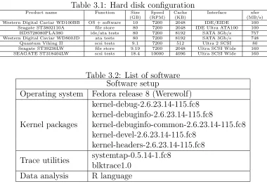
The platform is a custom desktop with a ASUS P4P800 motherboard, 2 Intel Pentium4 (Xeon) 3.00GHz processors and 512MB SDRAM. The operating system and all related software were installed on a 10 GB Western Digital Caviar WD100BB hard disk. This is connected directly to one IDE/ATA interface on the motherboard. Figure 3.1 shows the disk configuration.

The remaining disks were used for running tests. A Hitachi

(27)

Table 3.1: Hard disk configuration

Product name Function Size Speed Cache Interface xfer

(GB) (RPM) (KB) (MB/s)

Western Digital Caviar WD100BB OS + software 10 7200 2048 IDE/EIDE 100

Seagate ST3802110A file store 80 7200 2048 IDE Ultra ATA100 100

HDS728080PLA380 ide/ata tests 80 7200 8192 SATA 3Gb/s 757

Western Digital Caviar WD800JD ata tests 80 7200 8192 SATA 3Gb/s 748

Quantum Viking II scsi tests 9.1 7200 512 Ultra 2 SCSI 80

Seagate ST39236LW file store 9.19 7200 2048 Ultra SCSI Wide 160

SEAGATE ST318404LW scsi tests 18.4 10000 4096 Ultra SCSI Wide 160

Table 3.2: List of software Software setup

Operating system Fedora release 8 (Werewolf)

Kernel packages

kernel-debug-2.6.23.14-115.fc8 kernel-debuginfo-2.6.23.14-115.fc8

kernel-debuginfo-common-2.6.23.14-115.fc8 kernel-devel-2.6.23.14-115.fc8

kernel-headers-2.6.23.14-115.fc8 Trace utilities systemtap-0.5.14-1.fc8

blktrace1.0 Data analysis R language

Table 3.1 details the disk information.

To ensure that data does not get skewed by test result data different types of disks are used for storing data and running tests. If the tests are run on IDE/ATA disks the data is saved on the scsi backup disk and if the test is run on a scsi disk the results are stored on a SATA disk.

3.2 Measurement Methodology

Customization of blktap systemtap

For our measurements we modified and used the traceread.stp systemtap script. This file in its default form captures read I/O requests for all files to the traced block device or or to a specific file on the traced device. The file to be traced is passed as an argument to the systemtap script.

(28)

multiple files. This was set up in such a way that by specifying a command line sequence as a parameter, any file that began with this parameter could be traced.

The third modification was to disable the VFS layer traces. With the VFS layer tracing enabled a large amount of unnecessary VFS calls were being traced. This was making the system unstable and processing the data was becoming resource intensive.

The fourth modification was to print the name of the file that was being traced along with the other default block layer event information. This was needed to further help trace multiple files independently.

(29)

Measurements

The output generated by the blktrace systemtap scripts contains all the events that take place with respect to what is being traced. This includes information like plugging, unplugging, merging etcetera. For our measure-ment purpose we capture trace information associated wih theget request (G) , dispatch (D) and complete (C) block layer events.

When a BIO reaches the block layer it either gets merged into a existing block I/O request or a new block I/O request for it. Creation of a new block I/O request is a G operation. If a BIO gets merged there is no corresponding G request associated with it.

The following is an example of a block I/O request creation event.

0.223813758 0.000012802 G R sector 40871076, bytes 131072

We identify this block request uniquely by its sector number. In this case it is40871076. Between this event and the the time there could be requests which get merged to this request. For every G event we increment the OS queue by one.

When a event request gets dispatched to the disk the dispatch(D) event is captured. The following is an example of a sample D event.

0.224663367 0.000014380 D R sector 40871076 , bytes 262144

There are three things of note with this entry. The letter D indicates that it is a dispatch. The sector number identifies which request number is being dispatched. The third entry of interest is the number of bytes. In this case it is 262144. This is different from the number of bytes in the G entry above. This is because in between these two events there has been a new BIO got merged into this request and increased the size. When the D event happens we decrement the OS queue and increment the disk queue.

The last event of interest is the (C) event. This event marks the com-pletion of a block I/O request. The following is an example of a comcom-pletion event.

0.228458477 0.003795110 C R sector 40871076 , bytes 262144,

q2d 0.000862411 , d2c 0.003795110 , q2c 0.004657521

(30)

com-pleted. Theq2d entry signifies the time spent by the request on the os queue.

d2c signifies the time spent by the request on the disk queue. q2c signifies the total time spent (q2c = q2d + d2c) in servicing the request.

The disk queue is decremented by one when a C event occurs.

All our analysis and graphical display of I/O activity is based on these data captured from these three events.

3.3 Benchmarks

To study I/O behavior simple benchmarks were run to characterize I/O be-havior. The benchmarks perform one of intensive reads, writes or a combi-nation of both.

To negate the effect of the file system buffer cache the filesystem was unmounted and remounted before every test.

Single process sequential read

In this test a single 100MB file is read. The following command was executed and the block I/O details were captured. This was run for all the four schedulers and on a sata, ide/ata and a scsi disk.

cat /path/to/100MBFile > /dev/null

(31)

(32)

(33)

(34)

Two process sequential read

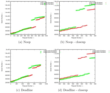
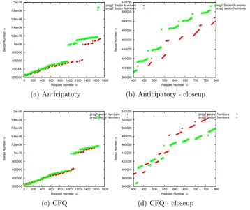
In this test two 100MB files are read concurrently. The following command was executed and the block I/O details were captured. This was run for all the four schedulers and on a sata, ide/ata and a scsi disk.

cat /path/to/100MBFile > /dev/null cat /path/to/2nd100MBFile > /dev/null

Our tool that analyzes the data generated by blktrace is able to identify I/O requests to specific unique files and we have graphically represented the I/O behavior of both the processes.

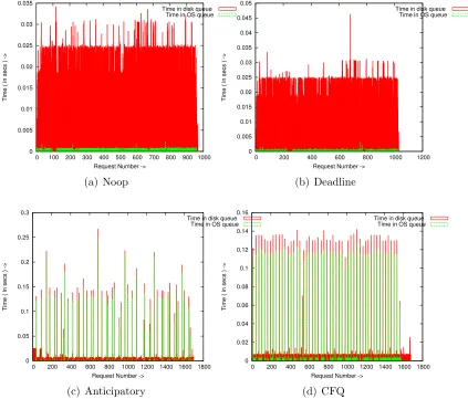
Here we start to observe significant significant differences in I/O behavior between the schedulers. Deadline and NOOP response times are almost that of CFQ and anticipatory. CFQ outperforms anticipatory by a small margin on scsi and ata.

From a response time perspective, CFQ and anticipatory, have very small OS queue time and disk dispatch times. Its on the the order of 3 - 4 mil-liseconds. Deadline and NOOP result in smaller os queue times. But the dispatch times are much larger ( to the order of 15 - 19 milliseconds).

Figure 3.6 illustrates the distribution of request queue times and request dispatch times for the four different schedulers. In the case of Noop and Deadline time spent on disk queue is more whereas for the Anticipatory and Deadline time spent in the OS queue is longer.

This essentially shows that Noop and Deadline, by scheduling requests immediately is causing heavy disk seeks and hence increased disk response time. On the other hand Anticipatory scheduling with its anticipation delay and CFQ with it proportional share behavior cause requests to collect and then dispatched to the disk. This improves on the response time.

(35)

Figure 3.1: Test platform disk configuration

0 50 100 150 200 250 300 350 400 450 500

0 0.5 1 1.5 2 2.5 0

0.5 1 1.5 2 2.5 3

Requests -> _{Queue size ->}

Time ( in secs ) ->

disk queue size Time in OS queue Time in disk queue os queue size

(36)

320 325 330 335 340 345 350

1.5 1.51 1.52 1.53 1.54 1.55

Requests ->

Time ( in secs ) ->

(a) Queue time

0 50 100 150 200 250

1 1.005 1.01 1.015 1.02 1.025 1.03 0 0.2 0.4 0.6 0.8 1 1.2 1.4

Time ( in secs ) ->

(b) Queue size

Figure 3.3: Queue time and size - closeup

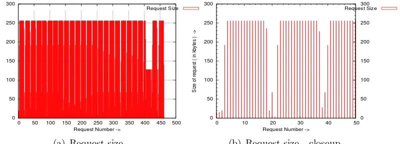
0 50 100 150 200 250 300

0 50 100 150 200 250 300 350 400 450 500

Size of request ( in kbytes ) ->

Request Number ->

Request Size

(a) Request size

0 50 100 150 200 250 300

0 10 20 30 40 50 0 50 100 150 200 250 300

Size of request ( in kbytes ) ->

Request Number ->

Request Size

(b) Request size - closeup

(37)

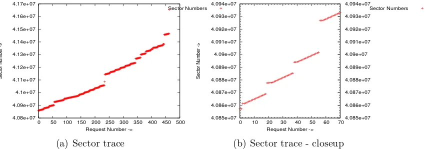
4.08e+07 4.09e+07 4.1e+07 4.11e+07 4.12e+07 4.13e+07 4.14e+07 4.15e+07 4.16e+07 4.17e+07

0 50 100 150 200 250 300 350 400 450 500

Sector Number ->

Request Number ->

Sector Numbers

(a) Sector trace

4.085e+07 4.086e+07 4.087e+07 4.088e+07 4.089e+07 4.09e+07 4.091e+07 4.092e+07 4.093e+07 4.094e+07

0 10 20 30 40 50 60 70 4.085e+07 4.086e+07 4.087e+07 4.088e+07 4.089e+07 4.09e+07 4.091e+07 4.092e+07 4.093e+07 4.094e+07

Sector Number ->

Request Number ->

Sector Numbers

(b) Sector trace - closeup

(38)

0 0.005 0.01 0.015 0.02 0.025 0.03 0.035

0 100 200 300 400 500 600 700 800 900 1000

Time ( in secs ) ->

Request Number ->

Time in disk queue Time in OS queue

(a) Noop 0 0.005 0.01 0.015 0.02 0.025 0.03 0.035 0.04 0.045 0.05

0 200 400 600 800 1000 1200

Time ( in secs ) ->

Request Number ->

(b) Deadline 0 0.05 0.1 0.15 0.2 0.25 0.3

0 200 400 600 800 1000 1200 1400 1600 1800

Time ( in secs ) ->

Request Number ->

(c) Anticipatory 0 0.02 0.04 0.06 0.08 0.1 0.12 0.14 0.16

0 200 400 600 800 1000 1200 1400 1600 1800

Time ( in secs ) ->

Request Number ->

(d) CFQ

(39)

200000 400000 600000 800000 1e+06 1.2e+06 1.4e+06 1.6e+06 1.8e+06 2e+06

0 100 200 300 400 500 600 700 800 900 1000

Sector Number ->

Request Number ->

prog1 sector Numbers prog2 sector Numbers

(a) Noop 400000 500000 600000 700000 800000 900000 1e+06 1.1e+06 1.2e+06

400 450 500 550 600 650 700 750 800

Sector Number ->

Request Number ->

(b) Noop - closeup

200000 400000 600000 800000 1e+06 1.2e+06 1.4e+06 1.6e+06 1.8e+06 2e+06

0 200 400 600 800 1000 1200

Sector Number ->

Request Number ->

(c) Deadline 400000 500000 600000 700000 800000 900000 1e+06 1.1e+06 1.2e+06

400 450 500 550 600 650 700 750 800

Sector Number ->

Request Number ->

(d) Deadline - closeup

(40)

200000 400000 600000 800000 1e+06 1.2e+06 1.4e+06 1.6e+06 1.8e+06 2e+06

0 200 400 600 800 1000 1200 1400 1600 1800

Sector Number ->

Request Number ->

prog1 Sector Numbers prog2 Sector Numbers

(a) Anticipatory 380000 400000 420000 440000 460000 480000 500000 520000 540000

400 450 500 550 600 650 700 750 800

Sector Number ->

Request Number ->

prog1 Sector Numbers prog2 sector Numbers

(b) Anticipatory - closeup

200000 400000 600000 800000 1e+06 1.2e+06 1.4e+06 1.6e+06 1.8e+06 2e+06

0 200 400 600 800 1000 1200 1400 1600 1800

Sector Number ->

Request Number ->

(c) CFQ 360000 380000 400000 420000 440000 460000 480000 500000 520000 540000

400 450 500 550 600 650 700 750 800

Sector Number ->

Request Number ->

(d) CFQ - closeup

(41)

(42)

0 500 1000 1500 2000 2500 3000

0 1 2 3 4 5 6 7 8 9 10 0 1 2 3 4 5 6 7 8

Time ( in secs ) -> anticipatory-ide1-4proc-cat.stapout

anticipatory-ide1-4proc-cat.stapout:disk queue size anticipatory-ide1-4proc-cat.stapout:Time in OS queue anticipatory-ide1-4proc-cat.stapout:Time in disk queue anticipatory-ide1-4proc-cat.stapout:os queue size

Figure 3.9: Queue time and queue size - four process sequential read

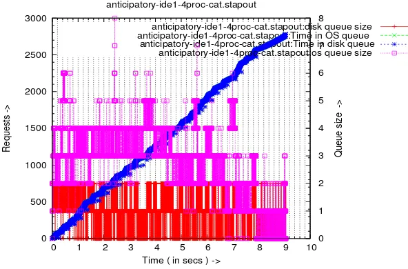
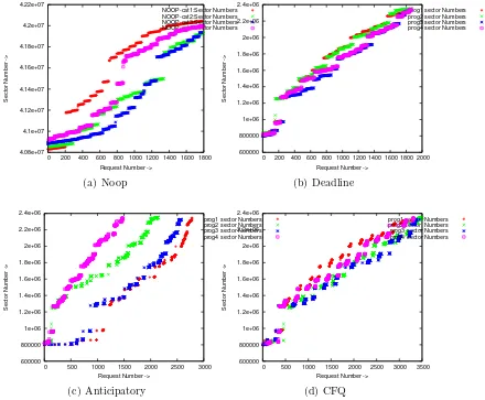
Four process sequential read

This is the same as the case with 2 processes. Instead of 2, we run 4 con-current read processes. The results are in line with the case of 2 concon-current processes. The effects however are more pronounced. Average response for anticipatory and CFQ requests lie in the 11 - 13 millisecond range whereas for deadline and NOOP it is close to 40 milliseconds. In terms of overall response time CFQ does marginally better on the scsi and the ide disk. The response time on the sata disk for CFQ and anticipatory are comparable. We also observe a marginal increase in the queue depths. This is illustrated in figure 3.9. The magenta and red linespoints represent os queue and disk queue.

(43)

4.08e+07 4.1e+07 4.12e+07 4.14e+07 4.16e+07 4.18e+07 4.2e+07 4.22e+07

0 200 400 600 800 1000 1200 1400 1600 1800

Sector Number ->

Request Number ->

NOOP-cat1:Sector Numbers NOOP-cat2:Sector Numbers NOOP-cat3:Sector Numbers NOOP-cat4:Sector Numbers (a) Noop 600000 800000 1e+06 1.2e+06 1.4e+06 1.6e+06 1.8e+06 2e+06 2.2e+06 2.4e+06

0 200 400 600 800 1000 1200 1400 1600 1800 2000

Sector Number ->

Request Number ->

prog1 sector Numbers prog2 sector Numbers prog3 sector Numbers prog4 sector Numbers

(b) Deadline 600000 800000 1e+06 1.2e+06 1.4e+06 1.6e+06 1.8e+06 2e+06 2.2e+06 2.4e+06

0 500 1000 1500 2000 2500 3000

Sector Number ->

Request Number ->

(c) Anticipatory 600000 800000 1e+06 1.2e+06 1.4e+06 1.6e+06 1.8e+06 2e+06 2.2e+06 2.4e+06

0 500 1000 1500 2000 2500 3000 3500

Sector Number ->

Request Number ->

(d) CFQ

(44)

Single process sequential write

In this test we write a single 100MB file to disk. The following command is executed and corresponding block layer I/O details were captured. dd if=/dev/zero of=/path/to/100MBfile bs=1M obs=8k count=100k

The observations here are a contrast from the read induced I/O of the previous benchmarks. Due to write back delay we see requests spending a large portion of the time on the os queue before getting dispatched. On an average the wait time ranges from 900ms in the sata disk to 1.2secs for the ide disk. The dispatch time for requests, however is in the range of 15 - 20 ms.

Because of the queue delay and the sequential nature of the I/O requests, a lot of requests get merged. It has been observed that each disk has a maximum request size. Once a requests’ maximum size is reached, adjacent requests do not get merged and a new request gets created. The sata and the ide disk have a maximum request size of 512KB bytes. For both the scsi disks the maximum request size attained was 384KB. Our understanding is that this limit is because of the scsi host adapter.

There is a substantial increase in the os and disk queue depths. The maximum os queue size for all devices under each scheduler was around 150. In case of the scsi disk, the disk queue maintained a size of 16. Native command queuing ( NCQ) was not enabled on the sata disks and hence the disk queue size of the sata and ide disks remained at 2.

Response times is comparable across schedulers. Across the disks the newer sata and ide disks perform better. We also believe that the LSI logic limits the scsi throughput.

(45)

0 20 40 60 80 100 120 140 160

0 0.5 1 1.5 2 2.5 0

20 40 60 80 100 120

Time ( in secs ) ->

(a) SATA 0 20 40 60 80 100 120 140 160 180

0 0.5 1 1.5 2 2.5 3 3.5 0 20 40 60 80 100 120

Time ( in secs ) ->

(b) SCSI

Figure 3.11: Queue depth and request times - single process streaming write

Two process sequential write & four process sequential

write

In the case of two process sequential write two 100MB files were written to disk concurrently. In the case of four process sequential write 4 100MB files were written to disk.

There was no major difference noted from our findings for a single read request. The total response time increases because the total amount of data written to disk increases. There is no significance difference in response times across different schedulers.

Two process sequential read and write

In this case two processes are run concurrently. One process does a sequential read of a 100MB file and the other process does a sequential write of another 100MB file.

(46)

the reads.

(47)

0 100 200 300 400 500 600 700 800 900

0 0.5 1 1.5 2 2.5 3 3.5 4 4.5 5 0 10 20 30 40 50 60 70 80 90

Time ( in secs ) ->

(a) i/o pattern

300 320 340 360 380 400

1.3 1.31 1.32 1.33 1.34 1.35 1.36 1.37 1.38 1.39 1.4 0 2 4 6 8 10 12 14 16 Requests ->

Time ( in secs ) ->

queue size Time in OS queue Time in disk queue os queue size

(b) i/o pattern - closeup

Figure 3.12: Anticipatory - i/o pattern of dd + cat

(48)

0 200 400 600 800 1000 1200

0 0.5 1 1.5 2 2.5 3 3.5 4 4.5 5 0 20 40 60 80 100 120

Time ( in secs ) ->

disk queue size Time in OS queue disk in disk queue os queue size

(a) i/o pattern

0 100 200 300 400 500 600 700 800 900

1.5 2 2.5 3 3.5 4

Requests ->

Time ( in secs ) ->

Figure 3.13: CFQ - i/o pattern of dd + cat

(49)

0 100 200 300 400 500 600 700

0 0.5 1 1.5 2 2.5 3 3.5 4 4.5 5 0 10 20 30 40 50 60 70 80 90 100

Time ( in secs ) ->

(a) i/o pattern

80 100 120 140 160 180 200 220 240

0.5 1 1.5 2 2.5 3

Requests ->

Time ( in secs ) ->

Figure 3.14: Deadline - i/o pattern of dd + cat

(50)

0 100 200 300 400 500 600 700

0 0.5 1 1.5 2 2.5 3 3.5 4 4.5 5 0 20 40 60 80 100 120

Time ( in secs ) ->

(a) i/o pattern

40 60 80 100 120 140 160 180 200

0.5 1 1.5 2 2.5

Requests ->

Time ( in secs ) ->

Figure 3.15: Noop - i/o pattern of dd + cat

(51)

Four process sequential read and write

In this case four processes are run concurrently. Two processes perform sequential reads on two different 100MB files. The remaining two processes perform 100MB writes onto different files.

The i/o characteristics are similar to the case of the two process test ( one read , one write). Anticipatory and CFQ distribute the read and write operations, whereas deadline and NOOP prioritize and dispatch the streaming write requests. In terms of response times, anticipatory and CFQ are comparable. Deadline and NOOP response times are comparable but their overall response times are more than the other two schedulers by about four seconds.

(52)

0 200 400 600 800 1000 1200 1400 1600 1800 2000

0 2 4 6 8 10 12 14 16 0 20 40 60 80 100 120

Time ( in secs ) ->

(a) Anticipatory 0 500 1000 1500 2000 2500

0 2 4 6 8 10 12 14 0 20 40 60 80 100 120

Time ( in secs ) ->

(b) CFQ 0 200 400 600 800 1000 1200 1400

0 2 4 6 8 10 12 14 16 18 0 20 40 60 80 100 120

Time ( in secs ) ->

(c) Deadline 0 200 400 600 800 1000 1200 1400 1600

0 2 4 6 8 10 12 14 16 18 0 20 40 60 80 100 120 140

Time ( in secs ) ->

(d) Noop

(53)

Single instance chunk read

The last set of benchmarks that we ran were the ones that do simultaneous chunk read operations. We open all files under some of the subdirectories of the kernel source directory. This operation simulates reading chunks of data from different locations within the disk. reads. We perform reads of all files under within particular directories

Chunk reads are performed by running find on a particular directory and reading all the files within that directory concurrently using multiple instances of cat.

The following command line was used to simulate chunk reads.

find /path/to/kernel/source -exec cat {} > /dev/null

The I/O patterns observed are quite different. First, the request size is small. The average request size is in the range of 10KB - 12KB. The total number of requests is much larger. There were approximately 3500 requests generated. OS and disk queue depths remain in the range of 0 - 2.

This test also causes the anticipatory scheduler to cause delays for all requests and hence results in a larger response time compared to the other schedulers. The CFQ scheduler response time is the shortest. Deadline and NOOP schedulers response times are comparable and their response times lies between those of CFQ and Anticipatory.

One interesting feature that is observed is that subsequent requests seem to cluster around. This is evident in the graph shown in figure 3.17. Figure 3.17a shows the overall requests for sectors. This appears to be constant but on doing a close up the clustering of requests becomes apparent.

Two instance chunk read

(54)

4.92e+07 4.94e+07 4.96e+07 4.98e+07 5e+07 5.02e+07 5.04e+07 5.06e+07 5.08e+07 5.1e+07

0 500 1000 1500 2000 2500 3000 3500 4000

Sector Number ->

Request Number ->

Sector Numbers

(a) Overall sector seek pattern

5.0404e+07 5.04045e+07 5.0405e+07 5.04055e+07 5.0406e+07 5.04065e+07 5.0407e+07 5.04075e+07

2600 2650 2700 2750 2800

Sector Number ->

Request Number ->

Sector Numbers

(b) Closeup sector seek pattern

Figure 3.17: Sector requests made by a single find - cat processes

Single instance chunk read + single instance sequential

read

This test comprised of performing chunk reads and sequential reads concur-rently. In the case of deadline and NOOP, there was an increase in response time for the sequential read operation. In the case of anticipatory and CFQ there was no latency noticed in the sequential read.

Single instance chunk read + single instance sequential

write

(55)

Chapter 4 I/O scheduler characterizations

In this chapter we use our test results to corroborate the motivation for the development of I/O schedulers.

4.1 I/O scheduler guidelines

The development of I/O schedulers has been based on making trade offs be-tween maximizing disk throughput and reducing latency & improving fair-ness. In addition, typical I/O characteristics affect the design of I/O sched-ulers. In this section we briefly explain some of these I/O characteristics.

Read requests are sensitive to latency. This is because of the

syn-chronous nature associated with reads. The application blocks on the request and continues after the request is completed. Writes’ on the other hand are essentially asynchronous and not latency sensitive.

Read requests are synchronous and tend to chunk. An application

makes a read request, waits for the operation to complete and then issues the next read request. Because of the synchronous nature of reads, requests are not streaming in nature. Concurrent read requests from multiple applications to multiple files will also not result in sequential block I/O requests.

Write requests are asynchronous and tend to stream. Writes

(56)

800000 900000 1e+06 1.1e+06 1.2e+06 1.3e+06 1.4e+06 1.5e+06 1.6e+06 1.7e+06 1.8e+06

0 50 100 150 200 250 300 350

Sector Number ->

Request Number ->

program:cat1 program:cat2

(a) dd I/O requests

600000 800000 1e+06 1.2e+06 1.4e+06 1.6e+06 1.8e+06 2e+06

0 200 400 600 800 1000 1200

Sector Number ->

Request Number ->

program1: dd program2: dd

(b) cat I/O requests

Figure 4.1: Comparison read and write I/O requests

are written to disk at a later stage by daemons like pdflush or kjournald. As a result write requests from multiple applications result in sequential and streaming block I/O requests.

Figure 5.1 illustrates the sequential nature of write requests. (Note: These diagrams are based on the noop scheduler which does request sorting based on sector numbers)

The read requests are generated by redirecting thecatoutput of a 100MB file to /dev/null.

cat 100MBfile > /dev/null

Write requests are generated by creating 100MB files using dd.

dd if=/dev/zero of=outfile bs=1M obs=8k count=100

Two instances of cat were run to generate the read requests. Two in-stances of dd were run concurrently to generate the write requests.

In fig 5.1a. the write requests from the 2 processes are interspersed in a sequential order. However, as seen in fig. 5.1b. the concurrent read requests does not result in sequential block I/O requests.

Disk latency is reduced by sequential access . Latency in disks

is due to disk seeks. If the stream of requests that are sent to the disk are sequential in nature, this in general, would result in sequential disk access for sectors and minimize disk seeks. On the other hand, non sequential requests would cause disk seeks and hence increase the latency.

Catch-22 situation. Latency sensitive reads result in non streaming

(57)

hand, non latency sensitive write requests cause sequential disk requests which improves disk latency.

4.2 NOOP

The current Linux 2.6 NOOP scheduler is essentially the original Linux 2.4 Linus I/O scheduler. This scheduler is designed to do I/O request ordering and merging. The goal is to minimize disk seeks. It worked on the principle of sorting requests based on sector numbers and merging adjacent requests. This type of scheduling results inmaximizing I/O throughputbut at the cost of being unfair and havinghigh request latency.

4.3 Deadline

The deadline scheduler was designed to overcome the two shortcomings of NOOP - read starvation and read latency.

Read starvation

Write requests being sequential in nature, can monopolize the dispatch queue. This can happen for two reasons. Firstly, if the read requests are at a higher sector address space - the scheduler will sort requests and the stream of write requests will get inserted ahead of the read requests. Secondly, the write requests tend to be sequential in nature and the scheduler is able to merge request.

(58)

dis-Table 4.1: Response times - Deadline Process Running Time

disk process anticipatory cfq deadline noop

SATA cat 4.95 4.76 4.56 4.55

dd 3.39 2.56 1.64 1.51

SCSI cat 6.87 5.31 7.01 7.02

dd 4.02 5.34 2.7 2.52

IDE cat 3.21 3.46 6.31 6.16

dd 3.63 3.53 2.71 3.54

patched. The blue dots to the left of the green stripes in figure 4.2a represent dispatching of read requests.

80 100 120 140 160 180 200 220 240

0.5 1 1.5 2 2.5 3

Requests ->

Time ( in secs ) ->

(a) Deadline 40 60 80 100 120 140 160 180 200

0.5 1 1.5 2 2.5

Requests ->

Time ( in secs ) ->

(b) Noop

Figure 4.2: Deadline overcoming the read starvation of Noop.

While deadline scheduler prevents starvation, our results don’t show any improvements in terms of read latency. The following is a comparison of read response time for the above example.

4.4 Anticipatory

Increased read latency

(59)

ad-Table 4.2: Response times - Anticipatory Process Running Time

SATA find-cat 9.11 8.38 12.87 12.94

cat 3.26 _2.52 7.44 7.52

SCSI find-cat 12.96 12.73 16.03 16.42

cat 4.11 _3.67 7.76 8.26

IDE find-cat 12.67 11.78 18.29 18.38

cat 2.31 _1.9 9.46 9.31

dress request latencies that can occur due to concurrent applications gener-ating read requests. Because of the read-wait-read nature of synchronous reads, the scheduler is alternating between requests from different appli-cations. This definitely causes high disk seeks and increases latency and response times.

The anticipatory scheduler addresses this problem by anticipating re-quests from a process for which it has dispatched the last request. This artificial wait in-turn results in improved overall response time and reduced latency.

Consider the example of running a sequential read program (cat) concur-rently with a chunk read program (find-cat). The chunk read induces high latency on the read program. This can be observed by checking the response times for deadline and the NOOP scheduler from the table below. When run under the Anticipatory scheduler, the read latency and response time is significantly reduced for the sequential read program.

(60)

0 500 1000 1500 2000 2500 3000 3500 4000 4500 5000

0 2 4 6 8 10 12 14

Anticipatory-cat:Time in OS queue Deadline-cat:Time in OS queue Deadline-findcat:Time in OS queue Anticipatory-findcat:Time in OS queue

(a) Queue time

150 200 250 300 350 400 450 500 550 600

1.2 1.25 1.3 1.35 1.4 1.45 1.5 1.55 1.6 Anticipatory-cat:Time in OS queue

Deadline-cat:Time in OS queue Deadline-findcat:Time in OS queue Anticipatory-findcat:Time in OS queue

(b) Queue time - closeup

Figure 4.3: Comparing the request queuing of one chunk-read (findcat) pro-cess and one sequential read(cat) propro-cess between the Anticipatory and the Deadline scheduler

4.5 Complete Fairness Queuing

The chunk read operation (find-cat), when run in isolation demonstrates a situation where the Anticipatory scheduler might anticipate requests from a process that no longer exists and cause an increase in overall response time when compared to running the same under the CFQ scheduler. From the timing information that we have collected for a single process find-cat and the two process cat-find we observe that the average time spent by a request in the OS queue is higher for the anticipatory scheduler. This happens because the scheduler is expecting a request from another process ( which in this case does not exist) and results in periods when no requests are dispatched to disk .

The following figures show the queuing behavior of the single chunk read process and the two process chunk read. This is done for Anticipatory and CFQ. We observe that in the single process chunk read Anticipatory has many periods of inactivity.

(61)

(62)

0 500 1000 1500 2000 2500 3000 3500 4000 4500 5000

0 1 2 3 4 5 6 7 8

CFQ-findcat:Time in OS queue Anticipatory-findcat:Time in OS queue

(a) Queue time

350 400 450 500 550 600 650 700

0.7 0.72 0.74 0.76 0.78 0.8 0.82 0.84 CFQ-findcat:Time in OS queue Anticipatory-findcat:Time in OS queue

Figure 4.4: Single process chunk read

0 2000 4000 6000 8000 10000 12000

0 2 4 6 8 10 12 14 16 18 Anticipatory-findcat2:Time in OS queue

Anticipatory-findcat:Time in OS queue CFQ-findcat2:Time in OS queue CFQ-findcat:Time in OS queue

(a) Queue time

5400 5500 5600 5700 5800 5900 6000 6100 6200 6300

8.4 8.45 8.5 8.55 8.6 8.65 8.7 Anticipatory-findcat1:Time in OS queue Anticipatory-findcat2:Time in OS queue CFQ-findcat:Time in OS queue CFQ-findcat2:Time in OS queue

(63)

Chapter 5 Observations and conclusion

In this section we summarize our observations and conclude.

With the help of the microbenchmarks and the analysis of the trace data we have been able to understand and observe I/O and I/O scheduler behavior. One key observation is that over time I/O schedulers developed from being ”work conserving” to being ”proportional share” Current generation I/O schedulers try to trade off maximum throughput with reducing latency ( specifically read latency) and in being fair.

In its attempt at reducing read latency, I/O schedulers dispatched read requests right away. And the OS queue depth for read requests is always small. There are instances when reads can get queued (E.g. the case of concurrent sequential read and chunk read). However, We have not observed read requests getting queued under these circumstances. Our understanding is that reads get queued in the I/O queues whereas writes can get queued in I/O as well as the dispatch queue.

(64)

be minimal.

In all our tests we have found the CFQ scheduler to be the most versatile. It has either matched or performed better than all the other schedulers under all environments.

The anticipatory scheduler performs well in almost all cases. While its main aim is to exploit deceptive idleness in read requests it has proved to be robust enough to handle issues related to starvation and read latencies.

The deadline scheduler does not have many advantages over the NOOP scheduler. It does avoid starvation but it does not perform any better than NOOP in reducing latencies.

(65)

Bibliography

[1] Bovet, D. and Cestati, M., .Understanding the Linux Kernel.,

[2] Corbet, J., .Linux Device Drivers

[3] Axboe, J., .Linux Block IO.Present and Future,. Proceedings of the Ottawa Linux Symposium 2004.

[4] Axboe, J., .Linux: Modular IO Schedulers ,.

http://kerneltrap.org/node/3851

[5] Corbet, J., .Modular, switchable I/O schedulers,. http://lwn.Articles/102926

[6] Iyer, S., and Druschel, P., .Anticipatory Scheduling: A Disk Scheduling Framework to Overcome Deceptive Idleness in Synchronous I/O,.SOSP 2001

[7] Pratt, S., Heger, D., Workload Dependent Performance Evaluation of the Linux 2.6 I/O Schedulers., Proceedings of the Ottawa Linux Sym-posium 2004

[8] Seelam, S., Romero, R., Teller, P., Enhancements to Linux I/O Schedul-ing., Proceedings of the Ottawa Linux Symposium 2005

[9] Blktrace Guide.,

https://secure.engr.oregonstate.edu/wiki/CS411/index.php/Blktrace Guide

[10] Brunelle, A., Block I/O Layer Tracing.,

(66)

[11] Systemtap Project Wiki., http://sources.redhat.com/systemtap/wiki/

[12] Systemtap tutorial., http://sourceware.org/systemtap/tutorial/systemtap.html

[13] Zanussi, Tom., Blktrace tapset., http://sourceware.org/ml/systemtap/2007-q1/msg00485.html

(67)

Appendix A

(68)

One process sequential read ( 1proc-cat)

Scheduler Request size Time in os queue Time in disk queue q2d + d2c

q2d d2c q2c

(Kbytes) (ms) (ms) (ms)

SATA

as 221 0.53 3.98 4.41

cfq 119 0.11 4.24 4.25

dl 221 0.51 4.03 4.44

noop 221 0.51 4.01 4.43

SCSI

as 192 0.37 6.81 7.02

cfq 118 0.05 6.66 6.55

dl 192 0.36 6.84 7.04

noop 192 0.38 6.84 7.05

IDE

as 203 0.46 4.72 5.07

cfq 116 0.14 2.77 2.84

dl 203 0.45 4.75 5.09

noop 203 0.46 5.02 5.36

Process Running Time

disk anticipatory cfq deadline noop SATA 2.11 2.1 2.12 2.12

(69)

Two process sequential read ( 2proc-cat)

q2d d2c q2c

SATA

as 147 3.06 4.6 7.55

cfq 121 3.39 3.58 6.89

dl 216 1.89 14.19 15.74

noop 201 2.77 14 16.45

SCSI

as 121 3.98 7 10.82

cfq 122 5.26 5.5 10.63

dl 199 0.49 22.81 22.76

noop 212 0.55 23.07 23.08

IDE

as 144 2.03 3.48 5.42

cfq 118 2.3 2.55 4.79

dl 196 4 15.69 19.32

noop 194 3.72 15.69 19.04

SATA cat1 4.27 4.41 7.26 7.42 cat2 4.52 4.29 7.28 7.37

SCSI cat1 6.81 6.35 10.12 10.18 cat2 6.57 6.01 10.11 10.21

(70)

Four process sequential read ( 4proc-cat)

q2d d2c q2c

SATA

as 147 9.19 4.41 13.5

cfq 121 8.44 3.63 11.98

dl 229 20.31 19.37 39.23

noop 229 20.7 19.75 39.99

SCSI IDE

as 148 7.79 4.17 11.86

cfq 117 6.15 2.76 8.85

dl 220 19.31 17.01 35.92

noop 219 19.74 17.43 36.76

SATA

cat1 8.19 8.37 16.99 17.31 cat2 8.84 8.61 17.01 17.35 cat3 7.33 8.38 16.99 17.25

cat4 8.79 8.4 17 17.34

SCSI

cat1 32.14 33.5 41.24 42.43 cat2 35.66 33.43 42.41 42.07 cat3 35.08 33.49 41.95 41.51 cat4 34.89 33.84 41.66 42.66

IDE

(71)

One process sequential write ( 1proc-dd)

q2d d2c q2c

SATA

as 476 947.08 22.62 969.16

cfq 468 972.83 23.44 995.72

dl 476 985.21 23.15 1007.82

noop 455 995.74 21.4 1016.64

SCSI

as 343 1214.69 166.59 1377.38

cfq 356 1236.49 203.17 1434.9

dl 347 1181.52 172.55 1350.03

noop 365 1203.57 216.88 1415.37

IDE

as 473 1247.6 28.39 1275.32

cfq 512 421.43 34.82 455.43

dl 476 1242.65 29.12 1271.09

noop 440 1248.86 27.47 1275.68

disk anticipatory cfq deadline noop SATA 1.61 1.44 1.51 1.48

SCSI 2.21 2.2 2.07 2.18

(72)

Two process sequential write ( 2proc-dd)

q2d d2c q2c

SATA

as 454 1040.34 22.21 1062.03

cfq 468 963.53 22.16 985.17

dl 463 1058.3 23.09 1080.85

noop 446 1020.84 21.6 1041.93

SCSI

as 330 1182.43 177.15 1355.42

cfq 322 1240.28 177.87 1413.98

dl

noop 333 1201.37 198.23 1394.96

IDE as

cfq 418 1330.58 26.58 1356.54

dl 439 1303.69 27.23 1330.28

noop 442 1310.08 27.04 1336.48

SATA dd1 4.05 3.72 3.92 4.02

dd2 4.2 3.8 4 3.91

SCSI dd1 4.42 7.34 5.44 6.5

dd2 6.56 6.67 6.89 6.42

IDE dd1 4.81 6.51 6.68 4.89

(73)

Four process sequential write ( 4Proc-dd)

q2d d2c q2c

SATA

as 407 1002.69 20.63 1022.84

cfq 417 934.35 21.06 954.92

dl 482

noop 414 1096.07 21.81 1117.36

SCSI

as 285 1102.68 157.26 1263.72

cfq 265 1095.86 155.17 1254.76

dl

noop 284 1168.92 171.68 1344.72

IDE

as 376 1171.47 22.98 1193.92

cfq 370 1283.17 23.69 1306.31

dl 367 1163.18 23.14 1185.78

noop

SATA

dd1 9.81 9.91 9.42 9.48

dd2 9.72 9.78 9.71 10.22

dd3 7.89 9.41 9.38 8.59

dd4 9.59 9.3 7.47 8.6

SCSI

dd1 18.07 26.98 30.23 29.27 dd2 27.32 31.83 30.95 30.6 dd3 31.05 31.81 30.22 34.27 dd4 30.31 32.98 30.23 23.66

IDE

(74)

Two process sequential read-write ( 2proc-ddcat)

q2d d2c q2c

SATA

as 182 225.23 6.97 232.04

cfq 178 271.51 6.48 277.83

dl 261 222.96 8.77 231.52

noop 280 232.38 8.74 240.92

SCSI

as 132 312.07 25.04 336.53

cfq 163 414.05 32.65 445.93

dl 233 341.82 60.73 401.12

noop 226 289.17 46.38 334.46

IDE

as 179 225.22 6.78 231.84

cfq 165 260.07 6.03 265.96

dl 241 294.77 11.02 305.52

noop 242 248.67 10.08 258.52

SATA cat 4.95 4.76 4.56 4.55

dd 3.39 2.56 1.64 1.51

SCSI cat 6.87 5.31 7.01 7.02

dd 4.02 5.34 2.7 2.52

IDE cat 3.21 3.46 6.31 6.16

(75)

Four process sequential read-write ( 4Proc-ddcat)

q2d d2c q2c

SATA

as 201 285.28 6.33 291.46

cfq 169 332.94 6.83 339.61

dl 279 315.56 17.95 333.1

noop 231 205.41 15.29 220.34

SCSI

as 151 390.03 27.12 416.52

cfq 159 324.79 34.35 358.34

dl

noop 250 390.88 81.99 470.95

IDE

as 173 249.9 6.78 256.52

cfq

dl 267 418.16 18.57 436.29

noop 329 585.36 22.3 607.14

SATA

cat1 5.83 6.2 12.92 13

cat2 5.71 6.19 13 12.92

dd1 8.81 8.91 5.21 4.45

dd2 8.69 8.5 4.82 4.54

SCSI

cat1 9.01 7.01 17.43 17.62 cat2 8.06 7.49 17.38 17.57 dd1 12.72 12.16 6.56 6.48

dd2 12.61 11 3.03 6.75

IDE

(76)

One instance chunk read ( find - cat )

q2d d2c q2c

as 13 0.18 0.45 0.62

cfq 10 0.06 0.42 0.47

dl 13 0.07 0.49 0.55

noop 13 0.07 0.5 0.55

disk process anticipatory cfq deadline noop SATA find-cat 7.08 5.85 6.02 6.08

SCSI find-cat 10.64 9.29 9.43 9.41 IDE find-cat 11.29 10.05 10.14 10.04

Two instance chunk read ( find - cat )

q2d d2c q2c

SATA

as 9 1.11 0.75 1.84

cfq 10 0.67 0.88 1.53

dl 12 0.14 1.84 1.93

noop 12 0.14 1.8 1.89

SCSI

as 9 1.11 0.75 1.84

cfq 10 0.67 0.88 1.53

dl 12 0.14 1.84 1.93

noop 12 0.14 1.8 1.89

IDE

as 10 2.02 2.06 4.03

cfq 11 4.18 5.32 9.37

dl 12 0.13 11.91 11.76

(77)

SATA find-cat1 16.3 13.06 13.84 13.5 find-cat2 16.33 13 13.56 13.43

SCSI find-cat1 23.16 22.08 32.79 32.95 find-cat2 23.49 22.1 32.88 32.85

IDE find-cat1 28.5 48.64 54.21 56.3 find-cat2 28.14 48.54 53.65 56.35

One instance chunk read and

one instance sequential read ( fc-cat )

q2d d2c q2c

SATA

as 33 0.73 1 1.71

cfq 27 0.73 0.83 1.54

dl 34 0.89 3.58 4.4

noop 34 0.83 3.6 4.34

SCSI

as 30 0.65 2.46 3.05

cfq 33 0.82 2.53 3.29

dl 35 0.11 4.96 4.95

noop 35 0.11 5.1 5.09

IDE

as 33 0.46 1.77 2.18

cfq 29 0.5 1.49 1.95

dl 34 1.34 5.15 6.37

(78)

SATA find-cat 9.11 8.38 12.87 12.94

cat 3.26 2.52 7.44 7.52

SCSI find-cat 12.96 12.73 16.03 16.42

cat 4.11 3.67 7.76 8.26

IDE find-cat 12.67 11.78 18.29 18.38

cat 2.31 1.9 9.46 9.31

One instance chunk read and

one instance sequential write ( fc-dd )

q2d d2c q2c

SATA

as 33 0.73 1 1.71

cfq 27 0.73 0.83 1.54

dl 34 0.89 3.58 4.4

noop 34 0.83 3.6 4.34

SCSI

as 27 57.69 7.3 64.82

cfq 29 63.47 8.01 71.29

dl

noop 30 55.41 11.86 66.99

IDE as

cfq 24 39.93 2.14 42.02

dl 27 40.5 2.53 42.97

(79)

SATA find-cat 9.71 8.66 8.56 8.72

cat 2.22 1.65 1.56 1.61

SCSI find-cat 14.31 13.14 13.24 12.99

cat 2.61 2.31 2.28 2.2

IDE find-cat 14.33 13.65 13.64 13.48

(80)

An Evaluation of Linux I/O Scheduler Behavior at the Block I/O Layer

ABSTRACT

BIOGRAPHY

TABLE OF CONTENTS

LIST OF TABLES

LIST OF FIGURES

Chapter 1

Introduction

1.1

Overview - I/O schedulers

1.2

Problem Description

1.3

Significance

1.4

Thesis Organization

Chapter 2

Background

2.1

Linux Block I/O layer

2.2

Linux I/O Schedulers

2.2.1

NOOP scheduler

2.2.2

Deadline scheduler

2.2.3

Anticipatory scheduler (AS)

2.3

Device plugging

2.4

Blktrace

2.4.1

Relay file system

2.5

Systemtap

2.5.1

blktrace tapset

Chapter 3

Experiments

3.1

Test bed

3.2

Measurement Methodology

Customization of blktap systemtap

Measurements

3.3

Benchmarks

Single process sequential read

Two process sequential read

Four process sequential read

Single process sequential write

Two process sequential write & four process sequential

write

Two process sequential read and write

Four process sequential read and write

Single instance chunk read

Two instance chunk read

Single instance chunk read + single instance sequential

read

Single instance chunk read + single instance sequential

write

Chapter 4

I/O scheduler characterizations

4.1

I/O scheduler guidelines

4.2

NOOP

4.3

Deadline

4.4

Anticipatory

4.5

Complete Fairness Queuing

Chapter 5

Observations and conclusion

Bibliography

Appendix A

One process sequential read ( 1proc-cat)

Two process sequential read ( 2proc-cat)