Efficient Rare Event Simulation Using DPR for
Multidimensional Parameter Spaces
Ahmet A. Akyama¸c
1, Zsolt Haraszti
2, J. Keith Townsend
1,3Abstract
Performance constraints in communication systems and networks require the error or fault probabilities to be very low. Analytical and numerical models are often too restrictive and Monte Carlo simulation is computationally prohibitive for low probabilities. Importance sampling (IS) has been used to estimate rare event probabilities but is increasingly difficult to apply to complex systems where there is an indirect relationship between the inputs and the system response. Splitting is an alternative rare event simulation method that can overcome some of the difficulties associated with IS techniques, and has produced satisfactory results for systems for which the splitting parameter space is one dimensional. However, when the efficient simulation of the rare event requires that splitting is controlled by multiple system parameters, incorrect choice of the splitting parameters can lead to estimates with poor statistical accuracy. In this paper, we show that the important regions of the multidimensional parameter space can be correctly and easily identified when the system parameters are selected depending to the nature of the rare event. The equalization of the raw or unweighted steady state probabilities within the important region yields statistically accurate rare event estimates. The probability equalization can be achieved using the readily available Direct Probability Redistribution (DPR) method, by mapping the multidimensional parameter space to a one dimensional DPR control parameter. In this paper, we discuss alternative ways to perform this mapping, and demonstrate multidimensional splitting using two illustrative example systems4.
I. Introduction
Performance constraints in communication systems and networks require the error or fault
proba-bilities to be very low. For example, in Asynchronous Transfer Mode (ATM) networks, the cell loss
and delay probabilities are typically required to be on the order of 10−9 and less. Thus, an important
phase in the design of systems and networks involves the determination of such rare event
probabil-ities. Due to the complexity of the systems involved, analytical and numerical models are often too
restrictive and Monte Carlo (MC) simulation is computationally infeasible for low probabilities.
Im-portance sampling (IS) has been used to estimate rare event probabilities in communication systems
and networks (see [1] for a survey on the application of IS to communication systems and networks).
In very complex systems, it is often difficult to determine effective IS methods due to the increasingly
indirect relationship between the modifiable parameters and the system response, which could lead to
poor statistical accuracy in the estimates. Due to this complexity, reevaluation for changing system
topologies involves reimplementing the IS method for each topology. Furthermore, if the relationship
between the modifiable parameters and the system response is not properly identified, improper use
of IS could result in the phenomenon of underestimation [2]. Thus, it is desirable to be able to employ
1
Center for Advanced Computing and Communication, Dept. of Electrical and Computer Engineering, North Carolina State University, Box 7914, Raleigh, NC, USA 27695-7914. Tel: +1 919 515 7353, Fax: +1 919 515 2285, Email: {aaakyama, jkt}@eos.ncsu.edu.
2Applied Research Lab - Switchlab, Ericsson Telecom AB, S-12625 Stockholm, Sweden. Tel: +46 8 719 2499, Fax: +46 8 719
6677, Email: [email protected].
3
Corresponding author.
4
a rare event simulation technique which is easy to implement and which can directly influence the
system response without suffering from poor statistical accuracy and underestimation.
Splitting can be viewed as an alternative approach to rare event simulation and can potentially
overcome some of the difficulties associated with IS. Splitting has been considered in early works
[3] and has recently been used in the context of queueing networks [4], [5], [6], [7], [8], [9], [10],
[11]. The main notion behind splitting is to partition the system states into subsets. When a subset
is entered during system simulation, numerous retrials are initiated with the current subset as the
starting or entry state of the system. Essentially, the main system trajectory is split into a number
of subtrajectories. The number of subtrajectories spawned after visiting each subset is determined by
the splitting or oversampling factors. The splitting method involves the selection of the subsets and
oversampling factors, where the subsets are indexed such that the higher subsets correspond to the
rare events. Splitting increases the relative frequency of the rare events by placing an emphasis on
higher subsets. Efficient splitting can be achieved by equalizing the steady state probabilities of the
subsets under splitting [5], [6], [9], [10]. A method of splitting called RESTART [4], [5] assumes the
subsets are nested, and allows for only single subset transitions in a trajectory, and assumes integer
oversampling factors. A more general technique we apply here, called direct probability redistribution
(DPR) [10] requires the subsets to be disjoint (but not necessarily nested), and accounts for multiple
subset transitions. The DPR technique can be used to estimate steady state probabilities in finite state
Markovian or semi-Markovian systems, and has been successfully applied to performance estimation
in mobile wireless systems [11] and in ATM systems [10], including ATM systems with internal flow
control and systems with multiple hops, for which traditional IS techniques are difficult to implement.
Existing splitting techniques typically use one system parameter to control the splitting (e.g., the
queue length). Thus, the state space is partitioned into subsets according to a singlesplitting parameter
that is often a directly observable system parameter. However, there are systems for which efficient
splitting cannot be achieved without using multiple system parameters when constructing splitting
subsets. These systems can be characterized in two ways: the rare events are related to multiple
system parameters, or the typical trajectories the system takes to the rare events are defined through
multiple system parameters. The time-reversal two node Jackson network with a two dimensional
system space, for which single-parameter splitting failed to yield statistical estimates in [8], falls into
the first category. We consider two illustrative example systems, which fall into either of the above
categories.
In this paper, we present a technique to implement multidimensional splitting. To use our technique
to obtain efficient and accurate statistical estimates of rare event probabilities, it is necessary to
perform the following: to select system parameters as splitting parameters that properly represent
to the occurrence of the rare event; and to set the splitting factors such that the raw steady state
probabilities in the important region are equalized. We use the termmultidimensional direct probability
redistribution to refer to the DPR simulation that performs the above three actions. Multidimensional
DPR is implemented by mapping the multidimensional parameter space to the subset indices that
control DPR simulation. We discuss alternative ways to perform this mapping and show that if the
mapping is not performed compliant to the typical trajectories the system follows to the rare events,
the resulting estimates will not be statistically accurate and may even exhibit the phenomenon of
underestimation.
We demonstrate multidimensional DPR with two illustrative example systems, the first of which is
the same two node Jackson network used in [8], and the second of which is a rate-controlled (leaky
bucket policed) ATM switch. We show in both cases that improper mapping of the multidimensional
parameter space to the subset indices results in estimates with poor statistical accuracy, and sometimes
in underestimation. We point out that, for these systems, the above problems occur when the system
trajectories that result from an improper choice of subsets are not the same as the typical trajectories
that lead to the rare event under normal circumstances. This behavior has been observed before in
earlier works on IS [2] and more recently in works on splitting [8].
We demonstrate that, in the case of splitting, the onset of poor statistical estimates and
under-estimation coexists with other simpler to detect symptoms, such as the lack of convergence of the
mean estimate and the non-decreasing relative error. Thus, we present guidelines on how to detect
the improper selection of splitting parameters and multidimensional mapping. For the two systems
considered, we then proceed to identify different splitting parameters that include the typical
trajec-tories that lead to the rare events. We also address other issues such as the determination of the
oversampling factors and the DPR-specific iterative exploration process used in the initial phase of the
DPR simulation.
The remainder of this paper is organized as follows: In Section II, we give an overview of the DPR
simulation technique, followed by a description and discussion of the calculation of the oversampling
factors in Section III. Multidimensional DPR and the mapping of multiple splitting parameters to the
DPR subset indices is presented in Section IV. The DPR simulation methodology and results for the
two-node tandem Jackson network and the rate-controlled ATM switch are presented in Sections V
and VI, respectively. We present concluding remarks in Section VII.
II. The DPR Simulation Technique
The DPR simulation technique was developed in detail in [10]. Here, we summarize some key results
and notations that will be used in the remainder of the paper. Note that this section introduces DPR for
a one-dimensional indexed subset partition. Multidimensional DPR will be described in the subsequent
Let the state space of the system be denoted byS and assume there are nstates, such that|S|=n,
where| · |denotes the cardinality of the set. The system state is defined by a set of system parameters
that are not necessarily statistically independent. For example, for a single queue fed by Markovian
sources, the queue length, source states and server state would be a set of system parameters. The
individual states are indexed from S ={1, . . . , n}. Let V0,V1,V2, . . ., Vk ∈ S represent the system
evolution, i.e. the states that are visited in successive observation points. Using DPR, the set S
is partitioned into m disjoint, nonempty, indexed subsets S1, . . . ,Sm. The partitioning is uniquely
defined by a subset indicator function:
Γ(Vk)∈[1, m] : Γ(Vk) =i⇐⇒Vk∈ Si (1)
The macro-evolution of the system can thus be represented by the series Γ(V0),Γ(V1),Γ(V2), . . ..
Let µ = {µ1, . . . , µm} denote the so-called oversampling vector, which defines the retrial or
over-sampling factors µi for each subset Si. We assume, without loss of generality, that µ1 = 1 and
µ1 ≤ µ2 ≤ . . . ≤ µm. If this condition is not satisfied, the subset indices described by Γ(·) can be
reordered according to µand normalized to form a set of indices described by a new subset indicator
function Γ0(·) such that µ01 = 1 and µ01 ≤ µ02 ≤ . . . ≤ µ0m. Subsequently, Γ0(·) would replace Γ(·)
as the subset indicator function. Using DPR, each subset Si is visited µi times more often than it
would have been using MC simulation [10]. Denoting the steady state probabilities of the original and
m-partitioned system by π = {π1, . . . , πn} and π(m) = {π
(m) 1 , . . . , π
(m)
n }, respectively, the following
relationship holds between πl and π
(m)
l :
πl(m)= Φ·µΓ(l)πl, for 1≤l≤n (2)
where Φ is a normalization constant, Φ = 1/Pnl=1µΓ(l)πl.
During DPR simulation, a trajectory is split whenever a transition to a higher indexed subset occurs,
e.g., the system makes a transition from subsetSi to subsetSj such that i < j. The expected number
of new subtrajectories generated upon such a transition isµj/µi−1. The life of the new sub-trajectories
is restricted by the following ticketing mechanism: At its creation, each subtrajectory is assigned a
ticket, Ω, which is an integer number such that i < Ω ≤ j. A sub-trajectory is terminated when
it attempts to make a transition to a subset Sl for which l < Ω. Tickets are assigned randomly to
the new trajectory with a distribution that maintains the proper oversampling ratios in every subset.
According to DPR theory [10] and assuming the above Si → Sj, i < j transition, such a distribution
is:
Prob{Ω =l| Si → Sj}=
µl−µl−1
µj/µi if i < l≤j,
0 otherwise.
Due to the oversampling, every state of subset Si is visited, in the asymptotic sense,µi times more
procedure simulate (k,Vk, Ω, µ,h, e, r, w)
/* Initial call: k = 0, V0: arbitrary, Ω = 1 , h=e=0, r=w= 0*/
while k≤kmax do
Vk+1 :=transition (Vk) /* Make state transition(s) */ if Γ(Vk+1)<Ω then /* Investigate resulting subset indicator */
return /* Return if indicator smaller than ticket */
hΓ(V
k+1) :=hΓ(Vk+1)+ 1 /* Bookkeeping for the new state */
eΓ(V
k+1):=eΓ(Vk+1)+ 1/µΓ(Vk+1) /* Weighted subset counter */
r:=r+ Λ(Vk) /* Bookkeeping for rare events */
w:=w+ Λ(Vk)/µΓ(V
k) /* Weighted event counter */
if Γ(Vk+1)>Γ(Vk) then /* Conduct retrials if indicator larger than previous */
ndone:= 1 /* Number of trajectories done */
for i= Γ(Vk) + 1 toΓ(Vk+1)do /* One loop for each type of ticket */
n:= an occurrence of RVY such that /* Set desired number of traj’s */
n∈N
+ and E[G] =µ
i/µΓ(V
k)−ndone. /* . . . issued with ticket Ω =i */
for j = 1 to n
hΓ(V
k+1) :=hΓ(Vk+1)+ 1 /* Bookkeeping for extra trajectory */
eΓ(V
k+1) :=eΓ(Vk+1)+ 1/µΓ(Vk+1)
r:=r+ Λ(Vk) /* Bookkeeping for rare events */
w:=w+ Λ(Vk)/µΓ(V
k) /* Weighted event counter */
simulate (k+ 1, Vk+1, i, h,e, r, w) /* Trajectory with given ticket*/
end
ndone:=µi/µΓ(V
k)
end end end end
Fig. 1. Pseudo-code of the recursive simulation controller.
counters in the simulation are updated by weighting by a factor of 1/µi when in subset Si, or 1/µΓ(V )
in general, where V is the current state of the system.
The pseudo-code in Fig. 1 summarizes the simulation procedure. In Fig. 1, the counter vector h
represents the number of unweighted or raw hits per subset, the weighted counter vector e represents
the hits per subset weighted by the oversampling factors, the counter r represents the number of raw
hits of the rare event (referenced by the rare event indicator function Λ(·) ∈ {0,1}), the weighted
counter w represents the rare event hits weighted by the oversampling factor of the current subset
Γ(Vk), and kmax represents the maximum simulation time.
Note that the above DPR simulation mechanism does not require the rare event region (i.e., the
state space region where the rare event occurs) to be located in a specific subset. In other words,
Γ(.) and Λ(.) are not necessarily related, even though their mutual relationship may have a strong
effect on the efficiency of the DPR simulation. This is particularly observable in systems for which the
one dimensional subset indicator function provides a means of applying DPR and, as will be seen in
Sections V and VI, this flexibility allows solutions for cases for which the rare event function fails to
work as an efficient indicator function.
III. The Oversampling Factors
As will be shown in Sections V and VI, the determination of the subsets depends on the system and
the desired performance measure. Once the subsets are determined, the oversampling vectorµ has to
be chosen prior to performing DPR simulations.
Provided that the splitting parameters have been properly selected to represent the typical paths the
system takes to reach the rare events, efficient and accurate estimates of the rare event probabilities
can be obtained by a DPR setting that equalizes the visiting probabilities of the subsets. This can
be achieved by an oversampling vector µ that is chosen such that the resulting unweighted or raw
subset probabilities are roughly equalized. We do not claim such a setting is optimal or asymptotically
efficient, but it is supported by empirical studies of diverse cases, such as the examples considered in
Sections V and VI. Similar observations were also made in [5], [6], [9], [10].
Equalized hit probabilities of the subsets can be achieved by using DPR and setting the factors inµ
according to the inverse of the estimated steady state probabilities. Denoting the latter by P1, . . . , Pm,
where Pi =ei/
Pm
i=1ei, µ can be constructed such that µk = (maxiPi)/Pk for 1 ≤ i ≤m. Although
this represents a tautology, we use the concept of iterative subset exploration to estimate such an
oversampling vector µ. We start with a simple MC simulation (corresponding to a DPR simulation
withµ=1) which provides relatively accurate estimates of the high probability subsets. Using only the
high subset probabilities that satisfy a loose confidence constraint, we produce the first oversampling
vector. Typically, assuming the subset indicator function is properly chosen, a subsequent run with
the new oversampling vector will give further details about the higher subsets and can be used to
generate the next oversampling vector. We repeat the above iterative exploration process until the
proper oversampling vector which covers all subsets is obtained.
A pseudo-code that summarizes the iterative subset exploration is given in Fig. 2, whereµirepresents
the oversampling vector at iteration i≥ 0, the function callsimulate(k,Vk,Ω,µ,h,e, r, w) represents
a DPR simulation as in Fig. 1, and the function callreorder(µ,Γ(·),h,e, r, w) represents the reordering
described in Section II that results in increasing oversampling factors for higher subsets. In addition,
hmin represents the loose confidence constraint such that only those subsets that have higher thanhmin
hits affect the calculation of the oversampling factors. Note that since the reorder(·) function changes
the subset indicator function Γ(·) and the oversampling vectorµ, the subset counter vectorsh,e, and
the rare event counters r, w are also reordered to correspond to the new subset indicator function.
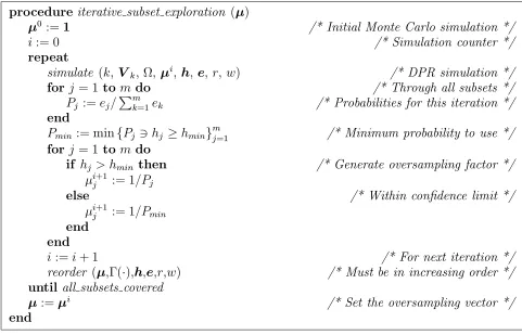
procedure iterative subset exploration (µ)
µ0 :=1 /* Initial Monte Carlo simulation */
i:= 0 /* Simulation counter */
repeat
simulate (k, Vk, Ω, µi,h, e, r, w) /* DPR simulation */
for j = 1 to m do /* Through all subsets */
Pj :=ej/
Pm
k=1ek /* Probabilities for this iteration */
end
Pmin := min{Pj 3hj ≥hmin}mj=1 /* Minimum probability to use */
for j = 1 to m do
if hj > hmin then /* Generate oversampling factor */
µij+1 := 1/Pj
else /* Within confidence limit */
µij+1 := 1/Pmin end
end
i:=i+ 1 /* For next iteration */
reorder (µ,Γ(·),h,e,r,w) /* Must be in increasing order */
untilall subsets covered
µ:=µi /* Set the oversampling vector */
end
Fig. 2. Pseudo-code of the iterative subset exploration.
show in Sections V and VI, the success or failure of the exploration process is strongly related to the
subset indicator function and, as such, can be regarded as a first indicator of the effectiveness of the
choice of the subset indicator function.
An alternative approach would be to use the results of the initial MC simulation and assume that
the tail is exponentially distributed to identify the oversampling factors for the higher subsets. The
exponential tail assumption holds in most cases where the tail is a large deviations (LD) tail. However,
some finite state systems may not have an LD tail or may not reach the LD tail within the subsets
of interest (e.g., the feedback system considered in [10]). The exponential tail assumption would not
be appropriate for such cases. The iterative subset exploration method provides a tail-independent
means of generating oversampling factors.
IV. Multidimensional DPR
Multidimensional DPR involves three steps. The first two steps are the determination of the multiple
splitting parameters, and the identification of the regions of the splitting parameter space that are
closely related to the occurrence of the rare event. The third is the mapping of the multiple splitting
A. Multidimensional Splitting Parameter Space
There are systems that require the use of multiple system parameters when constructing efficient
splitting subsets. These systems can be characterized in at least one of two ways: the rare events are
related to multiple system parameters, or the typical trajectories the system takes to the rare events
are defined through multiple system parameters.
To this end, let ω be the number of splitting parameters. Thus, the splitting parameter space is
ω-dimensional. Note thatωis not required to be the same as the dimensionality of the state spaceS of
the system. LetX = (X1, . . . , Xω) represent the splitting parameter space, the vectorx= (x1, . . . , xω)
represent a realization of the splitting parameters and letxk represent the splitting parameters at the
observation instant k. Each splitting parameter xi, 1 ≤ i ≤ ω can take on values xi ∈ Xi, where
|Xi| =di. For example, Xi could represent the queue length of a queue of size K, where di =K+ 1.
Thus, the number of possible realizations is given by Qωi=1di. Define I(x) ∈ {0,1} as an indicator
function of whether or not the realization xcontributes to the rare event, i.e. I(x) = 1 indicates that
x is a realization of system parameter for which either a rare event occurs or that is on a trajectory
that leads to a rare event. Thus, I(·) defines a region in the ω-dimensional parameter space that
contributes to the rare event. Obviously, I(x) ≡ 1 would include all realizations that contribute to
the rare event, but as we show in the Jackson network example in Section V, we can improve the
efficiency of the rare event simulation by selecting an I(·) that is more restrictive while maintaining
the realizations that include the rare event and the dominant paths to the rare event.
We hypothesize that ifx and I(x) are selected such that xcontains all system parameters that are
required to identify the important rare events andI(x) = 1 for all rare events and trajectories that lead
to the rare events (i.e., I(·) includes all rare events and trajectories that lead to the rare events), then
applying DPR such that the raw visiting probabilities are equalized among the realizationsxfor which
I(x) = 1 results in efficient and statistically accurate rare event probability estimates. Although we
do not present a formal proof of this hypothesis, it is strongly supported by the examples in Sections V
and VI.
B. Mapping of Splitting Parameters to Subset Indices
In order to apply DPR to the multidimensional splitting problem, we map the multiple splitting
parameters to a one dimensional subset indicator function to be used in DPR simulations. From
Section IV-A, the number of possible realizations of the splitting parameters is:
d1 X
x1=1 d2 X
x2=1
· · ·
dω
X
xω=1
I(x1, x2, . . . , xω)
Thus, a one-to-one mapping can be achieved by simply consideringm=Pdx11=1· · ·
Pdω
xω=1I(x1, . . . , xω)
accounts for multiple subset transitions [10] and the reordering of subsets (described in Section II)
guarantees a proper oversampling vector µ, this mapping will result in subsets that are suitable for
DPR simulation. Note, however, that such a mapping will also result in a large number of subsets.
For certain systems, a more efficient mapping can be found that reduces the number of subsets.
To this end, defineP(x) as the steady state probabilities of the realizationsx. Since the equalization
discussed in Section IV-A is achieved by assigning oversampling factors to the realizationsx that are
inversely proportional to P(x), the realizations with nearly identical oversampling factors can be
clustered to form one subset. Thus, a more efficient mapping would identify realizations x with
(almost) equal probabilities P(x) and cluster them to form one DPR subset. Essentially, the subsets
would be formed as isoprobabilistic clusters of realizations x.
The Jackson network in Section V is an example for which isoprobabilistic clustering can be
imple-mented, whereas the rate-controlled ATM network in Section VI is an example for which the one-to-one
mapping has to be implemented.
V. Two-Node Tandem Jackson Network
For the first case, we consider the two-node tandem Jackson network shown in Fig. 3. The input
into the network is Poisson distributed and has a rate λ. As indicated in [8], application of IS to this
system can be difficult. The first queue is of infinite size and has an exponential server with rateC1,
which feeds into the second queue, also of infinite size, which has an exponential server with rate C2.
Q1 Q2
C1 C2
λ
Fig. 3. The two-node tandem Jackson network.
We consider the rare event of interest to be the probability γk = Prob{Q1 ≥k, Q2 ≥ k}, where Q1
and Q2 represent the queue length in the first and second queues, respectively. Note that the state
of the system is defined by V = (Q1, Q2, α1, α2), whereαi is an indicator of whether serveri is busy.
We select the splitting parameter space defined by X = (Q1, Q2), which contains the rare events and
trajectories that lead to the rare events.
Setting λ = 1, C1 = 2 and C2 = 3, we form estimates ˆγk of γk for k ∈ {1,60}. We first show an
example of multidimensional mapping which results in an ineffective subset indicator function (also
used in [8]) . In this case, the poor statistical results are manifested as underestimation, as also noted in
[8]. We observe the onset of underestimation early on in the simulation by simple to detect symptoms.
Subsequently, we use a more refined mapping that is based on typical trajectories that lead to rare
A. Example of an Ineffective Indicator Function
The straightforward mapping for this system uses the rare event of interest. At any point (Q1, Q2)
in the two-dimensional splitting parameter space, we define Γ(Q1, Q2) = min{Q1, Q2}+ 1. This is
essentially the same subset indicator function used in [8].
We applied the iterative subset exploration method to generate the oversampling factors. However,
despite numerous iterations, the oversampling factors for the low probability subsets could not be
obtained because the simulation results were concentrated at the higher probability subsets. This was
the first indication of the problematic nature of the chosen subset indicator function. Nevertheless,
due to the exponential tail of the Jackson network, we used the exponential tail method described in
Section III to generate the oversampling vector.
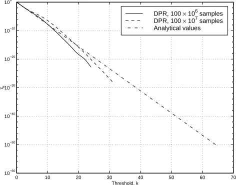
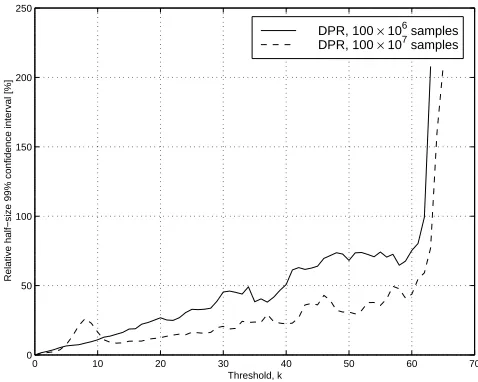
Using the above oversampling vector, we initially ran 100 sets of DPR simulations, each having a
duration of 106 simulation slots. The mean estimates ˆγk for 100 sets are shown as solid lines in Fig. 4
along with the analytical results, and the relative half-size 99% confidence intervals are shown as solid
lines in Fig. 5. The entire simulation took approximately 24 minutes on an IBM RS/6000 workstation.
It can be observed from Fig.’s 4 and 5 that the results are not statistically accurate, as apparent
from the difference in the estimates ˆγk with the analytical results for γk and the increasing confidence
intervals for k ≥10.
0 10 20 30 40 50 60 70
10−60 10−50 10−40 10−30 10−20 10−10 100
Threshold, k
γk
DPR, 100 × 106 samples DPR, 100 × 107 samples Analytical values
Fig. 4. Mean estimates ˆγk generated by DPR using subset indicator function Γ(Q1, Q2) = min{Q1, Q2}+ 1.
We subsequently increased the duration of the DPR simulations to 107 slots. The mean estimates
ˆ
γk and confidence intervals are shown as dashed lines in Fig.’s 4 and 5, respectively. Note that
the simulation results obtained by increasing the simulation time to 107 slots are inconsistent with
the ones obtained by using 106 slots. Furthermore, increasing the simulation time did not decrease
0 10 20 30 40 50 60 70 0
50 100 150 200 250
Threshold, k
Relative half−size 99% confidence interval [%]
DPR, 100 × 106 samples DPR, 100 × 107 samples
Fig. 5. Estimated half size confidence intervals (for 99% confidence level) normalized to the mean estimates, generated by DPR using subset indicator function Γ(Q1, Q2) = min{Q1, Q2}+ 1.
phenomenon of underestimation and are further indications of the problematic nature of the subset
indicator function.
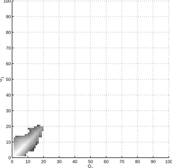
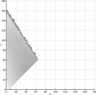
To better understand the problem behind the chosen subset indicator function, we present the
histogram of the visited states under a DPR simulation in Fig. 6, where the points with a high
number of hits are lightly shaded. It can be observed from the histogram in Fig. 6 that the choice of
0 10 20 30 40 50 60 70 80 90 100 0
10 20 30 40 50 60 70 80 90 100
Q2
Q1
Fig. 6. Histogram of visited states by applying min(Q1, Q2) + 1 as subset indicator (made from 107samples).
Γ(Q1, Q2) = min{Q1, Q2}+ 1 as the subset indicator function stresses the part of the state space for
which Q1 and Q2 are approximately equal. Most of the hits are concentrated along the line Q1 =Q2
and the regions closely surrounding it. This is mainly due to the fact that the subset indicator
increases when both queue lengths increase simultaneously. Thus, the DPR simulation reaches the
higher indexed (rare) subsets mainly through trajectories that are close to the line Q1 =Q2.
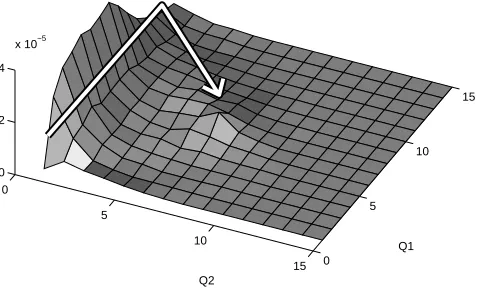
In Fig. 7, we plot the the typical paths followed by the system to rare event regions Ek
def
= {Q1 ≥
0
5
10
15 0 5
10 15
0 2 4
x 10−5
Q2
Q1
Fig. 7. A typical path that reaches Ekdef= {Q1≥k, Q2≥k} from (0,0) fork= 6.
E6 and demonstrate the preferred path of the system by an arrow in Fig. 7. This suggests that higher
subsets are reached through paths for which the first queue builds up to a certain level, and for which
the second queue builds up while the first one is draining. This is consistent with the observations made
in [8]. Note that these paths are not reflected in the trajectories that use Γ(Q1, Q2) = min{Q1, Q2}+ 1
as the subset indicator function.
The chosen subset indicator function reinforces numerous trajectories that do not coincide with
the natural trajectories of the system that lead to the rare events. Thus, the DPR simulation is
not computationally efficient and results in underestimation, as also indicated in [8]. On the other
hand, we were able to identify problems with the chosen indicator function both during the iterative
subset exploration process and the simulation process by observing the probability estimates and the
confidence intervals.
B. Refined Subset Indicator Function
For the Jackson network, the two dimensional probability mass function in the splitting space is an
inclined plane (in the logarithmic sense, and with different slopes in each dimension). Consequently,
the isoprobabilistic clusters are lines, which can be represented in one dimension using a mapping of
(Q1, Q2) to a subset indicator function of the form Γ(Q1, Q2) =bαQ1+βQ2+ 1c such that α/β <1.
The ratio α/βdetermines which queue is stressed more and the ratio being less than unity places more
stress on the second queue. The individual values of α and β determine the resolution of the subsets
in the low probability region.
Using preliminary simulation runs to equalize the stress on the two queues, we generated a ratio of
α/β = 1/1.5 and chose the following mapping:
Γ(Q1, Q2) =
Q1+ 1.5Q2
2
It is not surprising that this ratio is the same as the ratio of the service rates. The iterative subset
exploration method proved to be successful for all subsets using the above refined subset indicator
function.
Similar to the case in Section V-A, we ran two sets of simulations, the first one consisted of 100
batches of 106 simulation slots and the second one consisted of 100 batches of 107 slots. The mean
estimates ˆγk and confidence intervals are plotted in Fig.’s 8 and 9, respectively. The simulations took
53 min. and 523 min., respectively, on an IBM RS/6000 workstation.
0 10 20 30 40 50 60 70
10−60 10−50 10−40 10−30 10−20 10−10 100
Threshold, k
γk
DPR, 100 × 106 samples DPR, 100 × 107 samples Analytical values
Fig. 8. Mean estimates ˆγk generated by DPR using subset indicator function Γ(Q1, Q2) = (Q1+ 1.5Q2)/2 + 1.
0 10 20 30 40 50 60 70
0 50 100 150 200 250
Threshold, k
Relative half−size 99% confidence interval [%]
DPR, 100 × 106 samples DPR, 100 × 107 samples
Fig. 9. Estimated half size confidence intervals (for 99% confidence level) normalized to the mean estimates, generated by DPR using subset indicator function Γ(Q1, Q2) = (Q1+ 1.5Q2)/2 + 1.
As can be observed from Fig. 8, both the short simulations (solid line) and long simulations (dashed
line) result in consistent estimates which are almost identical to the analytical results. As expected, the
longer simulation run produces more accurate estimates, which is also apparent from the confidence
The stable behavior of the iterative subset exploration method, the consistent simulation estimates
and the confidence intervals are all indications that the refined subset indicator is a proper selection
and does not result in underestimation. Observation of the histogram of the visited states under DPR
simulation shown in Fig. 10 reveals that the refined subset indicator function includes the trajectories
that correspond to the typical paths the system takes to reach the low probability regions.
0 20 40 60 80 100 120 140 160 180 0
20 40 60 80 100 120 140 160 180
Q2
Q1
Fig. 10. Histogram of visited states with applying (Q1+ 1.5Q2)/2 + 1 as subset indicator (made from 107samples).
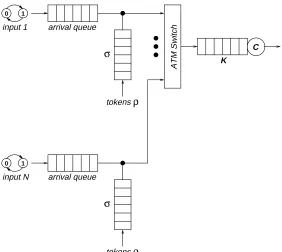
VI. Rate-Controlled ATM Switch
We consider the ATM switch with the leaky bucket rate controllers shown in Fig. 11. There areN
independent homogeneous input sources for which we define a triplet (p, m, b), wherepis the peak cell
arrival rate, m is the mean or sustained cell arrival rate and b is the mean burst length at the peak
rate. We assume the entire system is normalized with respect to the peak rate p and thus consider
time to be discrete, where one time slot corresponds to the arrival time of a single cell at the peak rate
p. With this normalization, we assume that, for each source, cells arrive according to an interrupted
Bernoulli process (IBP). The IBP sources can be in one of two states s∈ {0,1}and have a mean rate
of m and a mean burst length of b.
Each source is policed by a leaky bucket rate controller as shown in Fig. 11. The leaky bucket
controller consists of an arrival queue and a token queue. The token queue is of size σ and tokens
arrive at a rate of ρ, corresponding to a discrete-time (σ, ρ) shaper [12]. The arrival queue is assumed
to be sufficiently large such that cell loss at the arrival queue is negligible and peak rate control is
omitted since the model is normalized with respect to the peak rate. The cells exiting the shapers enter
an ATM switch with a shared bus switch architecture and are switched to the output queue, which
has a finite size ofK and a normalized service rate ofC = 1. We consider the queue length probability
mass function γx = Prob{Q = x}, which is rare for high values of x. The state of the system can
tokensρ
σ
tokensρ
σ 1
0
1 0
K C input 1
arrival queue
ATM Switch
arrival queue
input N
Fig. 11. ATM switch with leaky bucket rate controllers.
arrival queue length and token queue length of connection l, respectively, and Q is the output queue
length. For this system, we select the splitting parameter space defined by X = (B1, . . . , BN, Q),
which contains the rare events and trajectories that lead to the rare events.
Setting p = 1, m = 0.05, b = 10 for N = 8 sources and σ = 5, ρ = 0.05 for the leaky bucket
shapers and K = 40 for the output queue, we form estimates ˆγx for x∈ {1,40}. As in Section V, we
first use a mapping that results in an ineffective subset indicator function, which also leads to poor
statistical accuracy. We show that the problems with the indicator function can be detected by the
same symptoms used in Section V. We subsequently use a more refined mapping, again based on the
observation of typical trajectories that lead to rare events, which results in a subset indicator function
that produces statistically accurate estimates.
A. Example of an Ineffective Subset Indicator Function
For the rate-controlled ATM switch configuration, the straightforward mapping is of the form
Γ(B1, . . . , BN, Q) = Q, which focuses entirely on the output queue and is based on the rare event
of interest.
As was the case in Section V, we encountered difficulties in the iterative subset exploration process,
indicating that the chosen subset indicator function is problematic. Nevertheless, we used the best
possible version of the oversampling factors obtained from the iterative process. The best version is
considered to be the iteration that penetrates the highest subset.
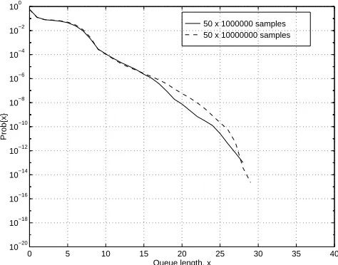
Using the oversampling vector, we ran 50 sets of two types of DPR simulations, with durations of
and dashed lines for 107 runs in Fig. 12. The relative half-size 99% confidence intervals are shown in
Fig. 13. The simulations took 86 minutes and 13 hours, respectively, on an Intel Pentium Pro PC
running FreeBSD Unix.
50 x 1000000 samples 50 x 10000000 samples
0 5 10 15 20 25 30 35 40
10−20 10−18 10−16 10−14 10−12 10−10 10−8 10−6 10−4 10−2 100
Queue length, x
Prob{x}
Fig. 12. Mean estimates ˆγx generated by DPR using subset indicator function Γ(B1, . . . , BN, Q) =Q.
50 x 1000000 samples 50 x 10000000 samples
0 5 10 15 20 25 30 35 40
0 50 100 150 200 250 300 350 400 450 500
Queue length, x
Norm. half conf.int.length (99%) [%]
Fig. 13. Estimated half size confidence intervals (for 99% confidence level) normalized to the mean estimates, generated by DPR using subset indicator function Γ(B1, . . . , BN, Q) =Q.
Even though analytical results are not readily available for this system, we can conclude from
Fig. 12 that the estimates are not consistent. This is due to the fact that, as seen in Fig. 12, the longer
simulation resulted in a probability curve that significantly deviates from the curve obtained from the
shorter simulation runs at low probabilities. Moreover, as seen in Fig. 13, the increase in the number
of simulation runs did not result in an observable improvement in the confidence intervals.
The above simulation observations, along with the difficulties encountered in the iterative subset
system, MC simulation trials indicate that the sum of the available tokens in the system affects the
typical paths to the rare events. We observed that the higher subsets are reached through paths for
which the token queues build up to a certain level, then begin to empty resulting in an increase in
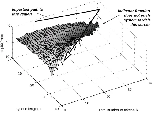
the output queue length. As can be observed from the histogram of the visited states under DPR
simulation in Fig. 14, these paths are not reflected in the trajectories that use Γ(B1, . . . , BN, Q) =Q
as the subset indicator function. In Fig. 14, the points with a higher number of hits are lightly
shaded. It can be observed from the histogram in Fig. 14 that the choice of Γ(B1, . . . , BN, Q) =Q as
0
10
20
30
40 0
10
20
30
40 -10
-5 0
Queue length, x Total number of tokens, k
log10(Prob)
Indicator function does not push system to visit this corner rare region
Important path to
Fig. 14. Histogram of visited states with applyingQas subset indicator (made from 107 samples).
the subset indicator function does not properly stress the token queues and results in most of the hits
being concentrated in regions for which the token queues are low.
B. Refined Subset Indicator Function
The probability surface for this system is not a plane and thus, the isoprobabilistic clusters are
not lines, as was the case in Section V. Since there is no obvious mapping from the two dimensional
splitting state space to a one dimensional subset index, we use a one-to-one mapping as described in
Section IV-B. However, in reference to the observations made from the MC trials, we use the sum
of the available tokens, PNi=1Bi, rather than the tokens available to the individual connections, since
the increase in queue length occurs depending on the sum of the tokens available in the leaky buckets.
The initial indexing of the subsets can be chosen arbitrarily maintaining a one-to-one relationship
between a point in the parameter space and a subset index, since this indexing will potentially change
for each step of the iterative subset exploration method which will reorder the subsets indices such
following mapping:
Γ(B1, . . . , BN, Q) = 41∗ N X
i=1 Bi
!
+Q (4)
The iterative subset exploration using the above initial subset indicator function was successful.
Using the oversampling vector from the iterative subset exploration, we again ran two sets of
simu-lations, consisting of 50 batches each of 106 and 107 simulation slots, respectively. The mean estimates
ˆ
γx and confidence intervals are plotted in Fig.’s 15 and 16, respectively. The simulations took 92 min.
and 13.5 hours, respectively, on an Intel Pentium Pro PC running FreeBSD Unix.
50 x 1000000 samples 50 x 10000000 samples
0 5 10 15 20 25 30 35 40
10−20 10−18 10−16 10−14 10−12 10−10 10−8 10−6 10−4 10−2 100
Queue length, x
Prob{x}
Fig. 15. Mean estimates ˆγx generated by DPR using the refined subset indicator function.
50 x 1000000 samples 50 x 10000000 samples
0 5 10 15 20 25 30 35 40
0 50 100 150 200 250 300 350 400 450 500
Queue length, x
Norm. half conf.int.length (99%) [%]
Fig. 16. Estimated half size confidence intervals (for 99% confidence level) normalized to the mean estimates, generated by DPR using the refined subset indicator function.
As seen from Fig. 15, the simulation runs are consistent in that the longer simulation refined the
for higher probabilities. The confidence intervals in Fig. 16 indicate that the longer simulation run
produced more accurate estimates, which is a further indication that underestimation did not occur.
Furthermore, note that the refined subset indicator function generated results for x ≤ 30 within a
100% relative confidence limit with 107 runs, whereas the straightforward indicator function was only
able to generate results for x ≤14 within the same confidence limit and for the same number of runs.
The histogram of the visited states under DPR simulation shown in Fig. 17 reveals that the refined
subset indicator function includes the typical paths to the rare events, as described above.
0
10
20
30
40 0
10
20
30
40 -10
-5 0
Queue length, x Total number of tokens, k
log10(Prob)
2D indicator function forces the system to visit this corner more frequently
Fig. 17. Histogram of visited states by applying the refined subset indicator function.
VII. Concluding Remarks
In this paper, we presented a splitting simulation technique for systems with multidimensional
parameter spaces. The technique, called multidimensional DPR, consists of two steps. The first of these
is the identification of the splitting parameters, and the second is the mapping of the multidimensional
parameter space to a one dimensional subset indicator function for use in DPR simulations.
Using our approach to obtain efficient and accurate statistical estimates of rare event probabilities,
it is necessary to perform the following: to select system parameters that properly represent the
rare event; to identify which regions of the multidimensional parameter space are closely related to
the occurrence of the rare event; and to set the splitting parameters such that the raw steady state
probabilities in the important region are equalized. We also discussed alternative ways to perform
the mapping of the multidimensional parameter space to a one dimensional subset indicator function
and showed that if the mapping is not compliant to the typical trajectories the system follows to
the rare events, the resulting estimates will not be statistically accurate and may even exhibit the
example systems, the first of which is a two node Jackson network, and the second of which is a
rate-controlled (leaky bucket policed) ATM switch. We observed, in both cases, that improper selection of
the mapping results in poor statistical accuracy. For the first system, we also observed the problem
of underestimation. We pointed out that, for these systems, the above problems occurred when the
system trajectories that result from an improper mapping are not the same as the typical trajectories
that lead to rare events under normal circumstances.
However, we demonstrated that the onset of poor statistical estimates and underestimation coexists
with other simpler to detect symptoms, such as the lack of convergence of the mean estimate and the
non-decreasing relative error. An advantage of the DPR technique is that it is flexible enough to be
quickly modified according to the underlying rare event mechanism of the investigated problem. Thus,
if a mapping is determined to be unsatisfactory, a relatively small effort is required to modify the DPR
simulation program to reflect a different choice of subsets. We subsequently applied different mappings
for the two systems which included the typical trajectories that lead to the rare events, which resulted
in statistically accurate simulations.
References
[1] P. Heidelberger, “Fast Simulation of Rare Events in Queueing and Reliability Models,” ACM Trans. on Modeling and Comp. Sim., vol. 5, no. 1, pp. 43–85, Jan. 1995.
[2] M. Devetsikiotis and J. K. Townsend, “An Algorithmic Approach to the Optimization of Importance Sampling Parameters in Digital Communication System Simulation,” IEEE Trans. Commun., vol. 41, no. 10, pp. 1464–1473, Oct. 1993.
[3] B. A. Bayes, “Statistical Techniques for Simulation Models,” The Australian Computer Journal, vol. 2, no. 4, pp. 180–184, November 1970.
[4] M. Vill´en-Altamirano and J. Vill´en-Altamirano, “RESTART: A Method for Accelerating Rare Event Simulations,” inProc. 13th Int. Teletraffic Congress, ITC 13 (Queueing, Performance and Control in ATM), Copenhagen, Denmark, June 1991, pp. 71–76.
[5] M. Vill´en-Altamirano et al., “Enhancement of the Accelerated Simulation Method RESTART by Considering Multiple Thresholds,” inProc. 14th Int. Teletraffic Congress, ITC 14, France, 1994, vol. 1a, pp. 797–810.
[6] P. Shahabuddin P. Glasserman, P. Heidelberger, “Splitting for Rare Event Simulation: Analysis of Simple Cases,” in1996 Winter Simulation Conference, Coronado, California, USA, December 1996, pp. 302–308.
[7] P. Glasserman, P. Heidelberger, P. Shahabuddin, and T. Zajic, “Multilevel Splitting for Estimating Rare Event Probabilities,” Tech. Rep. RC 20478, IBM Research Division, T. J. Watson Research Center, Jun. 1996.
[8] P. Glassermanet al., “A Large Deviations Perspective on the Efficiency of Multilevel Splitting,” Tech. Rep. RC 20691, IBM Research Division, T. J. Watson Research Center, Jan. 1997.
[9] P. Glassermanet al., “A Look at Multilevel Splitting,” Tech. Rep. RC 20692, IBM Research Division, T. J. Watson Research Center, Jan. 1997.
[10] Z. Haraszti and J. K. Townsend, “The Theory of Direct Probability Redistribution and its Application to Rare Event Simulation,” inProc. IEEE Int. Conf. Commun., ICC ’98, June 1998, pp. 1443–1450.
[11] Z. Haraszti, J. K. Townsend, and J. A. Freebersyser, “Efficient Simulation of TCP/IP for Mobile Wireless Communications Using Importance Sampling,” Submitted toIEEE MILCOM’98.