Fast FSR Methods for Second-Order Linear Regression Models

(1)

Abstract

CREWS, HUGH BATES. Fast FSR Methods for Second-Order Linear Regression Models. (Under the direction of Leonard Stefanski and Dennis Boos.)

Many variable selection techniques have been developed that focus on first-order

linear regression models. In some applications, such as modeling response surfaces,

fitting second-order terms can improve predictive accuracy. However, the number of

spurious interactions can be large leading to poor results with many methods. We focus

on forward selection, describing algorithms that use the natural hierarchy existing in

second-order linear regression models to limit spurious interactions. We then develop

stopping rules by extending False Selection Rate methodology to these algorithms.

In addition, we describe alternative estimation methods for fitting regression

mod-els including the LASSO, CART, and MARS. We also propose a general method for

controlling multiple-group false selection rates, which we apply to second-order linear

regression models. By estimating a separate entry level for first-order and

second-order terms, we obtain equal contributions to the false selection rate from each group.

We compare the methods via Monte Carlo simulation and apply them to optimizing

(2)

Fast FSR Methods for Second-Order Linear Regression Models

by Hugh Crews

A dissertation submitted to the Graduate Faculty of North Carolina State University

in partial fulfillment of the requirements for the Degree of

Doctor of Philosophy

Statistics

Raleigh, North Carolina

April 28, 2008

APPROVED BY:

Dr. Leonard Stefanski (Co-chair) Dr. Dennis Boos (Co-chair)

(3)

Dedication

(4)

Biography

Hugh Crews was born on March 1, 1982 in Wilmington, NC. After graduating from

New Hanover High School in 2000, he began his undergraduate work at North Carolina

State University in statistics. In May 2003, Hugh completed his Bachelor of Science

degree in statistics. After completing this degree, he decided to continue his graduate

work at NCSU. Hugh completed his Master of Statistics degree in May 2005 and

began working toward a doctoral degree. After finishing coursework, he began his

research under the direction of Dr. Leonard Stefanski and Dr. Dennis Boos. As a

college student, Hugh had the opportunity to teach an introductory statistics course,

advise undergraduates majoring in statistics, work on an air pollution problem with

(5)

Acknowledgements

First, I would like to thank my advisors Dr. Leonard Stefanski and Dr. Dennis Boos for

their guidance and support throughout my graduate career. As professors, they inspired

me to learn statistics, but as advisors, they challenged me to grow as a statistician.

I am thankful for my committee members who have taken time to contribute to my

research. I would also like to thank Dr. Bill Swallow who advised me through my years

as an undergraduate and convinced me to pursue a doctoral degree. I would also like

to thank the faculty and staff in the statistics department for making our department

a great learning environment.

I would like to thank SAS for employing me many summers and supporting me as

an undergraduate SAS Scholar. I would also like to thank GlaxoSmithKline for their

generous award which I received in my first year of graduate school. I must also thank

the National Science Foundation for supporting research in statistics.

I must thank Ben Ogorek for mentoring me in my first few years as a graduate

student. Without his help, I would not have grasped many of the key concepts in

statistics. I would also like to thank Clay Barker for mentoring me in the last few

years. He answered my numerous questions promptly and offered encouragement. His

support these last few years has gotten me through many tough situations. I would

like to thank Staples, Jeff, West, Brett, Brent, Scotty, Steve, and Jonah for running

with me throughout the years. I am grateful for Steve, Emily, David, Michael, McKay,

Darryl, and Joe, all of whom I met in graduate school. Finally, I must thank Mike,

(6)

college.

I must thank Marty Sugerik for introducing me to the field of statistics during my

time in high school. He was the first teacher to show me that mathematics has many

interesting applications.

Most importantly, I must thank my family for their support and encouragement

throughout my life. No matter what I pursue, they always show interest and support.

I am thankful for my brother and sister who always spend time with me when I visit

Wilmington. My father has been a great inspiration to me. He has always trusted

me to do what was best for myself and is always available for help, wisdom, and

(7)

List of Tables

Table 3.1 Example of Forward Sequence . . . 32

Table 3.2 Example of Alpha Grid . . . 35

Table 4.1 Forward Selection Step 1 . . . 42

Table 5.1 Methods and Stopping Rules . . . 57

Table 5.2 Method Abbreviations . . . 57

Table 6.1 Optimal Levels for Small Composite Design with 10 Factors . . . 81

Table 6.2 Optimal Levels for Central Composite Design with 8 Factors . . 81

Table 6.3 Variables in Cutinase Study . . . 85

Table 6.4 Model Summaries for Cutinase Production . . . 87

Table 6.5 Optimal Levels and Maximum Cutinase Production . . . 87

Table 6.6 Variables in Lipase Study . . . 88

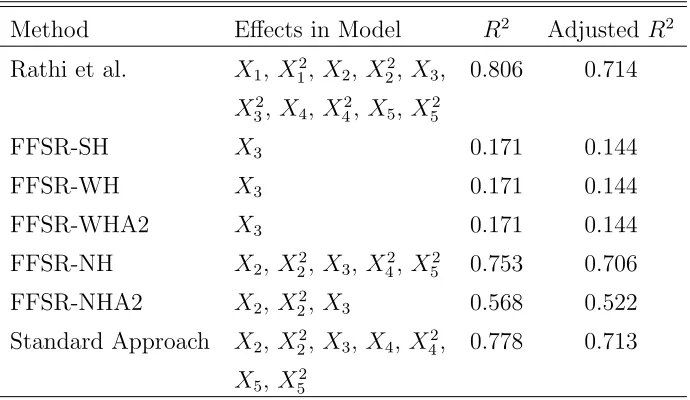
Table 6.7 Model Summaries for Lipase Production . . . 89

Table 6.8 Model Summaries for Specific Activity . . . 90

Table 6.9 Type III p-values for Rathi et al. Models . . . 92

Table 6.10 Optimal Levels for Maximum Lipase Production . . . 93

Table 6.11 Optimal Levels for Maximum Specific Activity . . . 93

(12)

Table 6.13 Model Summaries for Disease Progression . . . 95

Table 6.14 Variables in Pyrimidine Study . . . 97

Table 6.15 Variables in Pyrimidine Study Continued . . . 98

Table 6.16 Model Summaries for Pyrimidine Activity . . . 98

Table 6.17 Effects Selected for Pyrimidine Activity . . . 99

Table 6.18 Variables in Triazine Study . . . 100

Table 6.19 Variables in Triazine Study Continued . . . 101

Table 6.20 Variables in Triazine Study Continued . . . 102

Table 6.21 Model Summaries for Triazine Activity . . . 102

Table 6.22 Effects Selected for Triazine Activity . . . 103

Table A.1 Comparison of Methods: Normal Uncorrelated, Model 1, R2 _{= 0.25 . . . 113}

Table A.4 Comparison of Methods: Normal Correlated, Model 1,R2 _{= 0.25 116} Table A.5 Comparison of Methods: Normal Correlated, Model 2,R2 _{= 0.25 117} Table A.6 Comparison of Methods: Normal Correlated, Model 3,R2 _{= 0.25 118} Table A.7 Comparison of Methods: Chi Square Uncorrelated, Model 1, R2 _{= 0.25 . . . 119}

(13)

Table A.9 Comparison of Methods: Chi Square Uncorrelated, Model 3,

R2 _{= 0.25 . . . 121}

Table A.10 Comparison of Methods: Chi Square Correlated, Model 1,

R2 _{= 0.25 . . . 122}

R2 _{= 0.25 . . . 123}

R2 _{= 0.25 . . . 124}

Table A.13 Comparison of Methods: Normal Uncorrelated, Model 1,

R2 _{= 0.5 . . . 125}

R2 _{= 0.5 . . . 126}

R2 _{= 0.5 . . . 127}

Table A.16 Comparison of Methods: Normal Correlated, Model 1,R2 _{= 0.5} ₁₂₈

Table A.17 Comparison of Methods: Normal Correlated, Model 2,R2 = 0.5 . 129 Table A.18 Comparison of Methods: Normal Correlated, Model 3,R2 _{= 0.5 . 130}

R2 _{= 0.5 . . . 131}

R2 _{= 0.5 . . . 132}

(14)

R2 _{= 0.5 . . . 134}

Table A.23 Comparison of Methods: Chi Square Correlated, Model 2, R2 _{= 0.5 . . . 135}

Table A.24 Comparison of Methods: Chi Square Correlated, Model 3, R2 _{= 0.5 . . . 136}

Table A.25 Comparison of Methods for Model 1a . . . 140

Table A.26 Comparison of Methods for Model 1b . . . 141

Table A.27 Comparison of Methods for Model 2a . . . 142

Table A.28 Comparison of Methods for Model 2b . . . 143

Table B.1 Small Composite Design with 10 Factors (Runs 1-25) . . . 145

Table B.4 Orthogonal Central Composite Design with 8 Factors (Runs 1-25) . . . 148

(15)

List of Figures

Figure 3.1 Example of step function for model size by α. •indicates the closed lower bound for α corresponding to a specific model size.

◦indicates the open upper bound forα corresponding to specific model size. . . 33

Figure 3.2 Example plot of ˆγf ast(α) by α . . . 36

Figure 5.1 Correlation matrix for simulation study . . . 59

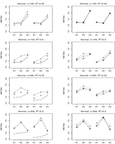
Figure 5.2 AME ratio (larger is better) using Normal predictors for LASSO

(L), FFSR-NH (N), FFSR-SH (S), FFSR-WH (W), FFSR-NHA2

(A), and FFSR-WHA2 (D). The first three values in each plot

are uncorrelated predictors and the last three values are

correlated predictors. . . 64

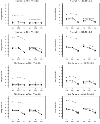
Figure 5.3 Average model size for LASSO (L), FFSR-NH (N), FFSR-SH

(S), FFSR-WH (W), FFSR-NHA2 (A), and FFSR-WHA2 (D).

The first three values in each plot are uncorrelated predictors and

the last three values are correlated predictors. . . 65

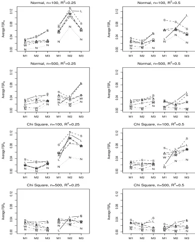
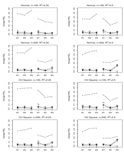
Figure 5.4 Average F SRm for LASSO (L), FFSR-NH (N), FFSR-SH (S),

FFSR-WH (W), FFSR-NHA2 (A), and FFSR-WHA2 (D). The

first three values in each plot are uncorrelated predictors and the

(16)

Figure 5.5 Average F SRq for LASSO (L), FFSR-NH (N), FFSR-SH (S),

FFSR-WH (W), FFSR-NHA2 (A), and FFSR-WHA2 (D). The

first three values in each plot are uncorrelated predictors and the

last three values are correlated predictors. . . 67

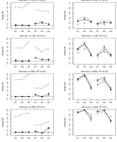
Figure 5.6 Average FSR (left) and CSR (right) using Normal predictors

for LASSO (L), FFSR-NH (N), FFSR-SH (S), FFSR-WH (W),

FFSR-NHA2 (A), and FFSR-WHA2 (D). The first three values

in each plot are uncorrelated predictors and the last three values

are correlated predictors. . . 68

Figure 5.7 Average CF for LASSO (L), NH (N), SH (S),

FFSR-WH (W), FFSR-NHA2 (A), and FFSR-FFSR-WHA2 (D). The first

three values in each plot are uncorrelated predictors and the last

three values are correlated predictors. . . 69

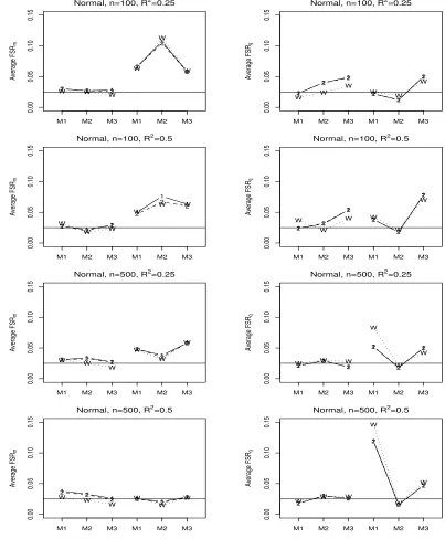
Figure 5.8 Comparison of average F SRm (left) andF SRq (right) using

Normal predictors for FFSR-NHA1 (1), FFSR-NHA2 (2), and

FFSR-WHA2 (W). The first three values in each plot are

uncorrelated predictors and the second three values are correlated

predictors. . . 76

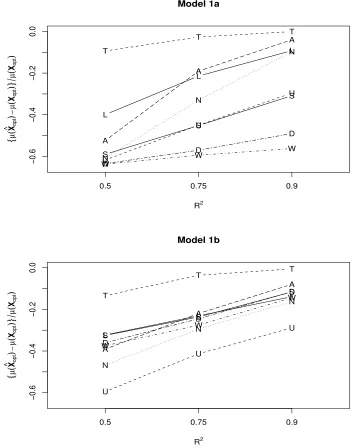
Figure 6.1 Scaled average difference in actual and optimal performance for

Model 1. True Model (T), Standard Approach (U), LASSO (L),

FFSR-NH (N), FFSR-SH (S), FFSR-WH (W), FFSR-NHA2 (A),

(17)

Figure 6.2 Scaled average difference in actual and optimal performance for

Model 2. True Model (T), Standard Approach (U), LASSO (L),

FFSR-NH (N), FFSR-SH (S), FFSR-WH (W), FFSR-NHA2 (A),

and FFSR-WHA2 (D). . . 84

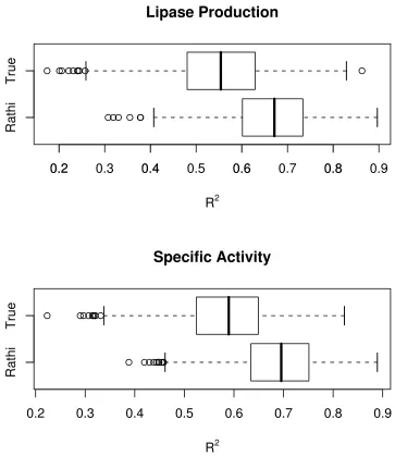
Figure 6.3 Boxplots of simulatedR2 _{values for lipase production and specific}

activity . . . 91

Figure A.1 AME ratio (larger is better) using Chi Square predictors for

LASSO (L), FFSR-NH (N), FFSR-SH (S), FFSR-WH (W),

Figure A.2 Average FSR (left) and CSR (right) using Chi Square predictors

for LASSO (L), FFSR-NH (N), FFSR-SH (S), FFSR-WH (W),

Figure A.3 Comparison of averageF SRm (left) and F SRq (right) using Chi

Square predictors for FFSR-NHA1 (1), FFSR-NHA2 (2), and

FFSR-WHA2 (W). The first three values in each plot are

uncorrelated predictors and the last three values are correlated

(18)

Chapter 1

Modeling Interactions in Regression

Analysis

1.1 Introduction

Suppose that a researcher is interested in developing a statistical model in order to

explain the variation in a response, Y, for some population of interest. The researcher is able to collect data onY andppredictorsX1, . . . , Xp for a set ofnindividuals. There

are two main goals that could be of interest. The first is understanding the relationships

between the response variable and the predictors, and the second is predicting future

observations. Putting this in statistical terms, the model of interest is

Y =f(X1, . . . , Xp) + (1.1)

where is random error and f(·) is a real-valued function, often a linear function of the predictors. In terms of this model, the first goal is obtaining an easily interpretable

estimate of f(·) that can be used in explaining the science behind the variation in the response. The second goal is obtaining the best prediction for f(·) at fixed values of the predictor variables. Depending upon the study at hand, the researcher may focus

(19)

Chapter 1. Modeling Interactions in Regression Analysis

A great amount of recent research has been done in the area of variable and model

selection in this regression setting. However, the focus of this paper is less on variable

and model selection, in general, and more on how to approach model selection in the

presence of interactions. Thus, some background information is omitted, and it is

assumed that the reader has basic knowledge of model selection techniques. However,

a brief discussion of the problem and a summary of the model selection methods can

be found in George (2000). For a more in-depth reference, refer to Miller (2002).

Much of the past research has been on simply choosing the best subset of

vari-ables in fitting the linear model f(X1, . . . , Xp) = β0 +Ppj=1βjXj. However, in the

real world more complex relationships between the response and the predictors exist.

Thus the next logical step in the model fitting process is to include all pairwise

in-teractions and quadratic effects, expanding the model of interest to f(X1, . . . , Xp) =

β0 +Ppj=1βjXj+P p

j≤kβj,kXjXk. Of course the three-way interactions, four-way

in-teractions, etc., could be added increasing the complexity of the problem. However,

merely including the second-order effects greatly increases the space of response

sur-faces and provides sufficient flexibility for fitting a variety of models.

1.2 Issues with Interactions in Regression

Since linear models are the most widely used and best understood regression models,

it is of interest to discuss how these methods handle interactions. We first describe

certain problems encountered when fitting linear regression models when interactions

are present. These problems reveal the two most common strategies currently employed

(20)

variable, whereas the second is to follow the natural ordering or “hierarchy” of the

terms. An in-depth description of these approaches highlighting their advantages and

disadvantages appears in later sections.

Interactions are often much harder to detect than main effects in regression

mod-eling. Multicollinearity, measurement error, the numerous forms interactions can take,

and lack of power for detection are all problems that make interactions troublesome.

Jaccard et al. (1990) suggest centering predictors to reduce multicollinearity. They

also argue that standardizing the predictors makes causal inference troublesome. The

remainder of their suggestions for dealing with interactions are based on proper

plan-ning of experiments and using prior knowledge or scientific theory to aid in the model

selection process. However, it is often the case that the researcher is doing exploratory

analysis and has very little prior information on which variables affect the response

in a simple manner, let alone as a complex interaction. Thus, automatic methods of

variable selection such as stepwise regression, best subsets, shrinkage methods, etc.,

are appealing. They aid in identifying possible informative variables before conducting

more controlled and costly studies or experiments.

Another issue that arises when fitting interactions is that significance tests are

not invariant to linear transformations of the data. The problem occurs with the

significance tests for main effects when corresponding second-order effects are also in

the model. Uncentered main effects are often correlated with their second-order effects,

and since this correlation changes depending upon the measurement units, the Type

III significance tests for the main effects change as well. Therefore, it is possible for

two researchers with the same data in different units of measurement using the same

(21)

Griepentrog et al. (1982). As a result, many statisticians recommend keeping main

effects in the model if their interaction is significant regardless of whether the main

effect is significant. This strategy is known as “maintaining the hierarchy” and is

often associated with backward elimination of terms. Another solution to the linear

transformation problem is to first standardize the predictors. If all researchers start

by standardizing the set of predictors, then they will always choose the same model

when applying the same method on the same dataset regardless of their choice of

measurement units.

The idea of maintaining the hierarchy leads to the two most popular approaches

in the model building process when interactions are of interest. The first is enforcing

the hierarchy and the second is not enforcing the hierarchy. Enforcing the hierarchy

means that when including interaction and quadratic terms in the model, we require

their parent main effects to be included as well. The remainder of this chapter is

organized as follows. The next section provides a short discussion on some commonly

used searching algorithms: best subsets, forward selection, backward elimination, and

stepwise regression. Then the approaches of enforcing the hierarchy and no hierarchy

are discussed using forward selection, as well as some issues that arise with each.

Finally, a “weak hierarchy” approach is discussed.

1.3 Subset Selection Methods

Many different strategies have been developed for searching through the possible

mod-els. We review the most basic and commonly used algorithms. “Best subsets” refers to

(22)

such as Mallows’ Cp, Adjusted R2, Akaike’s Information Criterion (AIC), Bayesian

Information Criterion (BIC), etc. The number of possible models, 2p_{, increases}

expo-nentially withp. Now consider including all the pairwise interactions and not enforcing the hierarchy. The number of total effects for a full quadratic is

pq = 2p+

p 2

, (1.2)

meaning that the number of subset models is 2pq. Even when enforcing the hierarchy,

the number of total subsets is large. Therefore, it should be obvious that unless p is very small, best subsets is impractical for searching models with interactions.

Forward selection starts with an intercept term and builds a model by adding terms

in a successive manner. At each step, the most informative variable is entered into the

model. The process continues entering variables until either all have been selected or

none meet the specified criterion for entry. Backward elimination starts with a full

model and removes uninformative variables one at a time. At each step a variable is

removed from the model until a stopping criterion is met or only an intercept term

remains. Backward elimination cannot be used when the number of possible terms

is greater than the sample size, which occurs more often when modeling interactions.

However, a solution to this problem is to use forward selection to build a large model

followed by backward elimination to “trim” it down. Another searching algorithm

combines forward selection with backward elimination at each step. This method,

called stepwise regression, is similar to forward selection in that in starts with an

intercept term and then builds a model. However, unlike forward selection, variables

(23)

most informative variable is entered or the most uninformative variable is removed

depending upon the criterion specified. The process proceeds one step at a time until

no variable meets the criterion for entry or removal. When including the pairwise

interactions, the number of total effects often outnumbers the sample size. For this

reason, forward selection and stepwise regression are obvious choices, since they can

be used when n < pq. The methods discussed and developed in this paper are applied

to forward selection, but they could be developed using backward elimination (when

n > pq) or stepwise regression.

1.4 No Hierarchy

Since it is often impossible to use best subsets or backward elimination, forward

selec-tion is commonly used. The simplest approach for fitting interacselec-tions using forward

selection is the no hierarchy approach where no restrictions are placed on the model.

Forward selection runs freely and can select any effect whether linear, quadratic, or

interaction regardless of the step in the model. That is, each term is a possible

candi-date for entry at the beginning of the forward selection process. Each term is treated

as a separate variable and selected according to the entry criterion.

There are three major problems with not enforcing the hierarchy. The first is

the tendency to choose larger and more complex models for a fixed α. As previously noted, each of the terms is treated as a separate variable, so that there arepq candidate

variables for entry on the first step. With so many more candidate variables at each

step, there is a higher expected number of selected variables than when only choosing

(24)

α entry-level =α0. Then for a model where none of the effects are truly important, the

probability for any single term to be entered is α0. When selecting from only p linear

terms, the expected model size is 1 +pα0, where 1 is added for the intercept. When

selecting from all linear, quadratic, and pairwise interaction terms at the beginning of

the selection process, the expected model size increases to 1 +pqα0. Also note that asp

grows, the pairwise interactions outnumber the linear terms, so there is a tendency to

choose them. Thus, not only are these models being overfitted, but they are often more

complex. A second problem with not maintaining the hierarchy is that the method

is not invariant to linear transformations of the predictors. However, henceforth we

suggest that the predictors be centered or standardized in order to avoid the lack of

invariance.

A third problem is that the quadratic or interaction effects and their corresponding

main effects are often highly correlated. This problem is greatly alleviated by centering

the predictors before creating the second-order terms. However, for highly skewed

pre-dictors, centering does not fully solve the problem. An alternative solution is sweeping

out the linear effects from each of the second-order effects and replace them with the

corresponding residuals. To sweep out the linear effects for quadratic terms, replace

X2

j with ˆ from the regression of Xj2 onto Xj. For interactions, replace XjXk with ˆ

from the regression of XjXk ontoXj and Xk.

1.5 Strong Hierarchy

A standard approach for finding informative interactions is to maintain the

(25)

then an interaction cannot be selected until both of its parent main effects are in the

model. Similarly, a quadratic term cannot be selected until its parent main effect is

in the model. Therefore, given the effects in the model, a candidate set of effects can

be formed. Only effects from this candidate set can be entered into the model. An

algorithm for forward selection with strong hierarchy is given below. Note that the

algorithm is limited to second-order terms.

1. Starting with an intercept term in the model, the candidate set includes all main

effects X1, . . . , Xp. Select the most informative effect from this set for model entry.

2. Suppose Xk is chosen in Step 1. Then the candidate set includes all remaining main

effects Xj, j 6=k and the quadratic effectXk2. Select the most informative effect from

this set for model entry.

3a. Suppose Xl is chosen at Step 2. Then the candidate set includes all remaining

main effects Xj, j 6=k and j =6 l, the quadratic terms Xk2 and Xl2, and the interaction

XkXl. Select the most informative effect from this set for model entry.

3b. Suppose Xk2 is chosen at Step 2. Then the candidate set includes all remaining

main effectsXj, j 6=k. Select the most informative effect from this set for model entry.

Proceed accordingly, adding new quadratic effects to the candidate set once their

par-ent main effect is selected and pairwise interactions once both parpar-ent main effects are

selected for the model.

Peixoto (1987) promotes using this practice of maintaining the hierarchy when

searching for the best model by forward, backward, or stepwise regression. He refers to

(26)

search-Chapter 1. Modeling Interactions in Regression Analysis

ing for such models. Stepwise regression would work just like the previous algorithm,

except at any given step a main effect cannot be removed unless there are no

second-order effects containing it currently in the model.

The advantage of the strong hierarchy is that it both enforces the hierarchy and

tends to choose smaller, less complex models since it does not select pairwise

interac-tions until both main effects have entered the model. The disadvantage of the strong

hierarchy is that there is no chance for important interaction terms to be included

unless both parent main effects are already in the model.

1.6 Weak Hierarchy

A less restrictive alternative to enforcing the hierarchy is to allow pairwise interactions

to enter the model once at least one of their parent main effects is included in the

model. Again, given the effects in the model, a candidate set of effects can be formed.

This method is employed in MARS (Friedman, 1991) and Penalized Logistic

Regres-sion (Park and Hastie, 2006). An algorithm for forward selection with weak hierarchy

is as follows. Note that the algorithm is limited to second-order terms.

1. Starting with an intercept term in the model, the candidate set includes all main

effects X1, . . . , Xp. Select the most informative effect from this set for model entry.

2. Suppose Xk is chosen in Step 1. Then the candidate set includes all remaining main

effects Xj, j 6= k, the quadratic effect Xk2, and all pairwise interactions of the form

XjXk, j 6=k. Select the most informative effect from this set for model entry.

(27)

main effects Xj, j 6= k and j =6 l, the quadratic effects Xk2 and Xl2, and all pairwise

interactions containing either Xk or Xl. Select the most informative effect from this

set for model entry.

3b. Suppose X2

k is chosen at Step 2. Then the candidate set includes all remaining

main effects Xj, j 6=k and all interactions of the form XjXk, j 6=k. Select the most

informative effect from this set for model entry.

3c. Suppose XlXk is chosen at Step 2. Then the candidate set includes all remaining

main effects Xj, j 6=k,the quadratic effect Xk2, and all interactions of the form XjXk,

j 6=k and j 6=l. Select the most informative effect from this set for model entry. Proceed accordingly, considering new quadratic effects once the parent main effect is

selected and pairwise interactions once either of the parent main effects is selected for

the model.

In terms of selecting interactions, the weak hierarchy approach provides a good

balance between enforcing the strong hierarchy and no hierarchy. The major weakness

of the strong hierarchy method is that it can miss important interactions, especially

in noisy models where both main effects are hard to detect. By making the selection

process less restrictive, the weak hierarchy suffers less in these cases. However, there is

no guarantee that all informative interactions will enter the candidate set early in the

selection process. The cost of making it easier for interactions to enter is that the weak

hierarchy still adds a large number of interactions to the candidate set. Therefore,

(28)

Chapter 2

Other Modeling Techniques

This chapter describes some alternative methods for estimating the regression function

f(X1, . . . , Xp). The first section is a short discussion of regression with shrinkage

focus-ing on the nonnegative garrote, the least absolute shrinkage and selection operator, and

some related methods followed by a discussion of recursive partitioning methods

lead-ing to Classification and Regression Trees. Finally, Multivariate Adaptive Regression

Splines that combines recursive partitioning with splines, is described.

2.1 Regression with Shrinkage

For some data sets, variable selection is not robust in the sense that small changes

in the data can result in very different models. Such instability can adversely affect

predictions. Therefore, alternative methods have been developed that are more stable.

Instead of estimating coefficients for a chosen subset of variables, these methods shrink

each variable’s coefficient. If some of the coefficients are shrunk to zero, then variable

selection is inherently conducted. In some sense, subset selection can be viewed as a

shrinkage method that selectively shrinks some coefficients to zero, while estimating

the others using ordinary least squares regression.

(29)

Chapter 2. Other Modeling Techniques

of squared beta coefficients when solving the normal equations. That is, it minimizes

n

X

i=1

(Yi−β0−

p

X

j=1

βjxij)2 (2.1)

subject to Pp_j₌₁β2

j ≤ s where s ≥ 0. Although ridge regression improves prediction

accuracy, its models are more difficult to interpret than subset selection methods since

ridge regression models retain all pq variables.

It is important to choose the right amount of shrinkage. For some variables the

estimates change drastically for different values of s. In general, the coefficients are shrunk more for small values of s than large values. A standard way to estimate s is though cross validation or generalized cross validation.

2.1.1 Nonnegative Garrote

One limitation of ridge regression is that it does not perform variable selection, and

therefore its models are often difficult to interpret. The nonnegative garrote (Breiman,

1995) was proposed in order to combine variable selection and shrinkage. It minimizes

n

X

i=1

(Yi−β0 −

p

X

j=1

cjβˆjolsxij)2 (2.2)

subject tocj ≥0 andPp_j₌₁cj ≤s. From (2.2) we see that the nonnegative garrote takes

the ordinary least squares estimates, ˆβols

j , and shrinks them using a different scaling

factor for each coefficient. Unlike ridge regression it shrinks some of the coefficients

to zero which leads to simpler models. The nonnegative garrote has predictive ability

(30)

In its original form, the nonnegative garrote enforces no hierarchy. Therefore, it

suffers from the same problems as forward selection with no hierarchy as described in

Chapter 1. However, adaptations of the nonnegative garrote have been developed to

handle interactions. Both the strong and weak hierarchy approaches have been applied

to the nonnegative garrote (Yuan et al., 2007b). With the strong and weak hierarchy

algorithms, main effects must be included in order for their interactions and quadratic

terms to be included in the model.

For the strong hierarchy, an additional constraint requires the scaling factor for a

quadratic term to be less than or equal to the scaling factor for its parent main effect.

Similarly, the scaling factor for an interaction must be less than or equal to both scaling

factors for its parent main effects. Let cj be the scaling factor for any main effect Xj

andcj,k be the scaling factor for a second-order termXjXk. Then the constraints imply

that cj,j ≤ cj for quadratic terms, and both cj,k ≤ cj and cj,k ≤ ck for interactions.

Any variable is included in the model if its scaling factor is nonzero. Therefore, with

the strong hierarchy imposed, any main effect cannot have scaling factor equal zero if

the scaling factor for any of its second-order terms is nonzero.

For the weak hierarchy, the constraint is changed so that for interactions the scaling

factor must be less than or equal to the sum of the scaling factors for its parent main

effects. That is, if XjXk is an interaction in the model, thencj,k ≤cj+ck. As a result,

any interaction in the model must have at least one of its parent main effects with a

(31)

2.1.2 Least Absolute Shrinkage and Selection Operator

The least absolute shrinkage and selection operator (LASSO) (Tibshirani, 1996) also

combines variable selection and shrinkage. The LASSO works by constraining the sum

of absolute beta coefficients when solving the normal equations. It imposes an L1

penalty on the least squares estimate, whereas ridge regression imposes an L2 penalty.

That is, the LASSO minimizes (2.1) subject to Pp_j₌₁|βj| ≤ s for some s ≥ 0. Like

the nonnegative garrote, the LASSO can shrink some of the coefficients to zero. An

advantage of the LASSO is that it avoids the ordinary least squares estimates that can

be adversely affected by multicollinearity.

The LASSO is a special case of least angle regression (LARS) (Efron et al., 2004).

Under a simple modification, LARS can be used to obtain the LASSO solution. Like

the nonnegative garrote, constraints can be added in order to achieve strong or weak

hierarchy with LARS (Yuan et al., 2007a). Some other extensions of the LASSO include

SCAD (Fan and Li, 2001) and the Adaptive LASSO (Zou, 2006) which both modify

the penalization constraint.

2.2 Recursive Partitioning

2.2.1 Automatic Interaction Detection

Tree-based regression techniques trace their heritage to the method called Automatic

Interaction Detection (AID) (Morgan and Sonquist, 1963). The basic idea of the

method is very simple: partition or split the data set into groups of similar responses

(32)

real-value a creates the groups Xi ≤ a and Xi > a. These groups or nodes are also

called tL and tR respectively. For each predictor, there exists at most n−1 of these

binary splits that result in different groupings of the actual observations. The goal is to

choose these splits to best explain the variation in the response. The basic algorithm

is given below.

1. Start with a single group ts containing all observations. Define the unexplained

variation for a group t as

R(t) = X

Xi∈t

(Yi−Yt)2 (2.3)

For ts, R(ts) =P_in₌₁(Yi−Yts)

2 _{is the total sum of squares.}

2. Split the data into two groups, tL and tR, that minimize the sum of squared errors.

That is, search all predictors for the binary split such that

∆R =R(t)−R(tL)−R(tR) (2.4)

is maximized.

3. Make sure that the reduction is greater than 1% of the total sum of squares. That

is, ∆R >0.01Pn_i₌₁(Yi−Yt)2. If not, then stop the splitting process.

4. Of the two groups,t1andt2, select the grouptwith the largest unexplained variation.

Search all possible nonoverlapping splits and choose the one that maximizes (2.4). Split

the group if the reduction, ∆R, is greater than 1% of the total sum of squares.

5. Continue searching and splitting groups until no group is more than 2% of the total

sum of squares.

(33)

in that group. That is,

b

Yt=n−t1

X

Xi∈t

Yi. (2.5)

Sonquist (1969) notes that AID is analogous to the sequential use of one-way

Anal-ysis of Variance (ANOVA) where the goal is to split the data into groups whose means

explain as much of the variation within the group as possible. He suggests the use of

AID to identify important interactions, but still recommends the use of scientific theory

to avoid interactions that make no sense. In response to this suggestion, Staelin (1970)

promotes the use of Tukey’s test for additivity to test for the presence of interactions.

Although AID was met with much enthusiasm, it was by no means flawless. Doyle

(1973) noted that:

1. By splitting the data, larger sample sizes are necessary to achieve high power

to detect effects.

2. Multicollinearity leads to spurious results.

3. Selection bias is created when building a model using a forward searching algorithm.

4. Selection bias is highly affected by noise such as measurement error in the

predic-tors.

5. Skewed predictors can lead to spurious results.

Like many others, he suggests the use of AID as an exploratory tool to help the

re-searcher specify the form of the model. Similar to forward, backward, and stepwise

regression techniques, AID also suffers from the problem that significance testing using

(34)

selec-Chapter 2. Other Modeling Techniques

tion or the amount of smoothing for splines, the 2% stopping rule for AID is arbitrary.

A later addition to the algorithm is limiting the minimum size of a final node, which

is an arbitrary choice as well. Based on these issues, much of the research for

extend-ing tree-based methods involves the process of “growextend-ing an honest tree.” The basic

elements of tree-based prediction include selecting the variables to use for splitting,

how to split, deciding when to stop growing the tree, and determining a method for

prediction once the tree is grown. For more history of AID and an updated version

called SEARCH refer to Morgan (2005).

2.2.2 Classification and Regression Trees

There have been numerous developments to resolve the issue of how to grow regression

trees. A popular method called Classification and Regression Trees (CART) (Breiman

et al., 1998) makes use of the original AID algorithm but approaches the problem by

growing overly large trees and then pruning them based on a cross-validation approach.

CART chooses binary splits of the data like AID, but CART proceeds until every final

node has a sample size of at most nmin. By choosing a small value for nmin, typically

nmin = 5, R(t) is often minimized. The largest tree grown using this stopping rule is

referred to as Tmax.

Despite having the “smallest” unexplained variation, Tmax is an overgrown tree

and needs to be pruned. In order to form subtrees, splits are deleted by remerging

the subgroups into a single group in a backward sequential fashion. Since nodes are

nonoverlapping, they cannot be removed alone or there will be holes in the prediction

(35)

choosing the final tree. This measure is defined as

Rλ(t) =R(T) +λ|Te| (2.6)

where λ is a complexity parameter and |Te| equals the number of final subgroups of the tree. Rλ(t) can be thought of as unexplained error plus a penalty for complexity.

Given a sequence of λ values, 0 = λ1 < λ2 < . . . , define Tk as the smallest subtree

that minimizes Rλ(T) for λk < λ < λk+1. Note that as λ increases, smaller trees are

favored.

In order to choose the best tree from the resulting sequence of subtrees, honest

estimates of R(Tk) are needed. This is done with V-fold cross validation. The process

works by randomly dividing the data into V subsamples, L1, . . . , LV, such that each

subsample has the same number of observations (or as close as possible). For v = 1, . . . , V, create the training sample that includes all observations not in Lv, and the

validation sample, Lv. The training sample is used to grow and prune the particular

tree, and the validation sample is used to estimate R(tk). After repeating this process

for all v, the average of each R(tk) is taken, resulting in the V-fold cross validation

estimate. This can also be defined as,

RCV_(T

k) =n−1 V

X

v=1

X

(Xi,Yi)∈Lv

(Yi−Y

(v)

(Tk))2. (2.7)

whereY(v)(Tk) is the mean for the terminal node corresponding to observationi in the

(36)

of Tmax that minimizes RCV(Tk). Define this value as

RCV_(T

k0) =minkR

CV_(T

k). (2.8)

However,Tk0 may not have a significantly lower value forR

CV _{than smaller trees. Since}

smaller trees are easier to interpret and therefore favored, the final tree chosen is the

simplest tree whose estimate from (2.7) is within one standard error ofRCV_(T

k0). That

is, the actual selected tree is the smallest tree such that

RCV(Tk)≤RCV(Tk0) +SE(R

CV

(Tk0)) (2.9)

where SE(RCV_(T

k0)) is the standard error of the estimate from (2.8).

Understanding the importance of the variables chosen in the splitting process is

an important issue. The measure of importance employed in CART is ∆R. That

is, the variables that reduce the sum of squared errors the most are deemed the most

important. CART uses the basic idea from AID, but implements an intelligent strategy

for choosing the right-sized tree for interpretation and prediction. Breiman et al. (1998)

emphasize that CART is one method for fitting regression models, but like any other

method requires “intelligent and sensible application.”

2.2.3 Chi Square Automatic Interaction Detection

Another method for growing regression trees called Chi Square Automatic Interaction

Detection or CHAID (Perreault and Barksdale, 1980) makes use of Bonferroni adjusted

(37)

to the 1% rule in the original AID algorithm. Unlike AID and CART, which only

permit binary splits, CHAID allows multiple splits of a single node. This provides

more practical and interpretable results, especially for nominal predictors which can

often be divided into more than just two distinct groups.

The CHAID algorithm works in the following way. The process begins by

deter-mining the number of splits that best describe each predictor. This is accomplished by

a process of merging levels of the predictor based on similar response patterns and then

splitting them if necessary. Note that if the predictor is continuous, then it must first

be partitioned into levels. That is, the researcher must choose ranges of the predictor

that make useful groups. The partitioning must be done in such a way that any value

of the predictor will fall into only one range. The grouping process starts by a pairwise

comparison of each level, merging those that are not significant based on a Chi-Square

test. After merging is done, the final group(s) can also be split. The advantage of this

additional process is that only predictors that are best described by more than one

group are then considered for actually splitting the dataset. Once the number of splits

is determined for each predictor, a Bonferroni-adjusted Chi-Square test is conducted

for each eligible predictor. The adjustment helps deal with the issue of selection bias

where predictors with more possible splits are favored. Assuming at least one of the

tests is significant, the predictor with the smallest p-value is then chosen. The dataset is then divided based on the splits of that predictor from the grouping process. After

splitting the dataset, the process is then repeated for each subgroup. Once all groups

are too small to be split or no predictors are significant from the Chi-Square tests, then

the process ends. Like AID, the predicted value for each final subgroup is the average of

(38)

diagram of the process, refer to Perreault and Barksdale (1980). Extended Automatic

Interaction Detection (XAID) (Heymann, 1981) is an extension of the CHAID

algo-rithm to better handle continuous predictors. It employs two sample t-tests rather than Chi-Square tests in the merging process.

Using Chi-Square testing in a forward, semi-hierarchical manner is reminiscent of

forward hierarchical regression presented in Chapter 1. One of the issues akin to such

searching procedures is the problem of inference using the final model. However, a

com-putational algorithm that calculates bootstrap standard errors for the predictions and

their corresponding confidence intervals has been developed (van Diepen and Franses,

2006).

Computer applications for CHAID and XAID are provided via a program called

Formal Inference-based Recursive Modeling (FIRM) (Hawkins, 1999). The

documen-tation for the two algorithms, called CATFIRM and CONFIRM respectively, describes

the main issues of recursive partitioning and the differences between FIRM and CART.

2.2.4 Other Techniques

Regression trees can be divided into two main groups: trees that use binary splits and

trees that use multilevel splits. AID and CART are in the former group whereas CHAID

and XAID are in the latter. There is a long list of similar methods that advance these

two basic approaches. QUEST (Loh and Shih, 1997) is a multistage inference-based

algorithm for fitting binary trees. By using multiple stages of testing in the variable

selection process, selection bias is reduced. GUIDE (Loh, 2002) uses Chi-Square tests

(39)

bias. Another important aspect of GUIDE is the inclusion of a Chi-Square test for

detecting pairwise interactions. CRUISE (Kim and Loh, 2001) uses multilevel splits,

linear combination splits, and GUIDE’s interaction test to produce less complex trees

with low selection bias. Finally, LOTUS (Chan and Loh, 2004) is an algorithm for

fitting logistic regression trees. Many more partitioning or tree-based algorithms exist,

most of which deal with the issue of selection bias.

So far, the trees grown use the mean of each terminal node as the prediction for

that group. However, other methods exist that make use of other estimators. Treed

regression (Alexander and Grimshaw, 1996) grows less complex binary trees than the

previously discussed methods. Instead of using the mean for prediction, the best simple

linear regression of the group using one predictor is alternatively fit, and predictions

are made using it. The goal of treed regression is to create less complex, more easily

interpreted tree models.

A resampling method for increasing the accuracy of regression trees was developed

by Brieman (1996). The method, called bagging, takes bootstrap samples from the

original sample, and then grows regression trees using them. Finally it takes the average

of the bootstrap predictors as the final predictor. Random Forests (Brieman, 2001)

generalizes the idea of growing a large number of trees through resampling techniques.

Brieman (2001) proves, via the Strong Law of Large Numbers, that as the number of

trees grown increases, the final estimate converges to the right-sized tree and thus does

not overfit. Although resampling methods can improve accuracy of predictions, they

complicate the model interpretation.

A shrinkage method for growing regression trees is discussed in (LeBlanc and

(40)

the LASSO in order to both prune branches of the tree and shrink the node estimates.

2.3 Multivariate Adaptive Regression Splines

As previously discussed, much of the need for automatic model selection techniques is

for researchers who are unable or unwilling to specify the form of the regression model.

Although recursive partitioning methods prove useful in detecting complex

interac-tions, they do not produce continuous models and have trouble handling simple linear,

additive, or interaction models of lower order. In fact, they cannot produce an additive

model with more than one main effect. Unlike partitioning methods, splines produce

continuous function estimates. Splines are a powerful nonparametric regression

tech-nique used to estimate smooth functions without specifying the form of the model.

However, they suffer from the need for high-dimensional basis functions to estimate

even simple functions. Multivariate Adaptive Regression Splines (MARS) was

devel-oped by Friedman (1991) in order to combine the adaptability of partitioning with the

smoothness of splines. In this section, an overview of MARS and some enhancements

to it are presented. For a review of spline estimation, refer to Eubank (1999).

The first step in understanding MARS is to see its relationship to the recursive

partitioning methods previously discussed. The partitioning methods were simply

de-scribed as splitting the data into subregions and then making predictions locally for

each terminal node. This lead to the tree-based view referred to as regression trees.

However, the partitioning methods can also be written as the sum of products of

in-dicator functions and regression coefficients. The inin-dicator functions identify the path

(41)

functions, the partitioning methods can be viewed as stepwise regression procedures,

where the goal is to find a set of basis functions whose corresponding estimator best

describes the data. Suppose there are m= 1, . . . , M subregions. Then,

b

f(X) =

M

X

m=1

amBm(X) (2.10)

wheream is the corresponding estimator for themth subregion. Bm(x) is the mth basis

function defined by

Bm(X) =I[X∈Rm] (2.11)

with Rm representing the terminal region of interest. The right hand side of (2.11)

can be broken further into the product of the Km indicator functions which give the

direct path to the specific region of interest. In order to see this, suppose that Xj is

the predictor used in the splitting process, and τ is the splitting point or knot. Also define,

Sk,m=

      

1 if right path,

−1 if left path

(2.12)

Then,

Bm(X) = Km

Y

k=1

I{Sk,m(Xj(k,m)−τk,m)≥0} (2.13)

where Sk,m tells which path, left or right, to take to get to a particular node, and

(Xj −τk,m) tells the path that the observation takes. If these paths match, then the

indicator function evaluates to 1. Otherwise, it evaluates to 0. Thus, by taking the

product of these indicators, the resulting basis is itself an indicator as specified in

(42)

In order to generalize the procedure, MARS substitutes the qth _{order spline basis}

function [Sk,m(Xj(k,m)−τk,m)]q+ for the indicator function I{Sk,m(Xj(k,m)−τk,m)≥0}

in (2.13). This leads to multivariate spline basis functions which take the form

Bq

m(X) = Km

Y

k=1

[Sk,m(xp(k,m)−τk,m)]q+. (2.14)

The advantage of using such basis functions is that if q > 0, they lead to continuous estimates of the regression surface. Taking q = 0 in equation (2.14) yields (2.13), i.e. the usual regression tree.

One of the major drawbacks of partitioning techniques is that simple functions

are not handled well. This is a direct consequence of limiting splitting to only

cur-rently terminal nodes. As the level of splitting increases, the degree of the interaction

increases, yielding models with higher order interactions. In order to overcome this

problem, MARS allows all basis functions, whether parent or daughter, to be

consid-ered throughout the selection process. For example, to fit a purely additive function,

the parent basis can be chosen multiple times using different variables. As a result,

MARS can handle linear, additive, and other simple functions as well as more complex

interactions and nonlinear models.

Except for q = 0, the product of two basis functions involving Xj does not yield a

spline basis of power q. In order to solve this problem, a final addition to the MARS procedure is that a basis cannot be split on the same variable more than once. Instead

the same basis and variable combination can be chosen multiple times to introduce

additional terms without increasing the level of splitting.

(43)

pro-Chapter 2. Other Modeling Techniques

ceeds in a forward stepwise fashion building a large set of basis functions to

approxi-mate the overall model. Like CART, MARS employs this forward step followed by a

backward deletion. However, instead of deleting whole splits, MARS is able to delete

specific basis functions if they are deemed unnecessary. This is due to the fact that the

parent basis is not deleted to create daughter bases. Instead, the parent is maintained

and considered again in the selection process. A consequence is that the basis functions

overlap and can be removed individually without leaving holes in the predictor space.

Once MARS chooses a set of basis functions the model, can be rewritten from the

form in (2.10) to a more interpretable form. Using an ANOVA-like decomposition, the

estimator can be broken up into a constant basis, plus basis functions involving only

one variable, plus basis functions involving two variables, and so forth. By rearranging

the terms in such a manner the estimator is defined as

b

f(X) =a0+

X

Km=1

fj(Xj) +

X

Km=2

fj,k(Xj, Xk) +

X

Km=3

fj,k,l(Xj, Xk, Xl) +. . . . (2.15)

Using (2.15), it is easy to see which variables interact and to what degree. This makes

for much easier interpretation than was present with regression trees.

Although there are many more specific details on the MARS procedure, such as its

cost complexity function, knot optimization, etc., they are excluded, and the reader

is referred to Friedman (1991). Some advancements to MARS include POLYMARS

(Kooperberg et al., 1997), which is a customized version used for fitting logistic

re-gression models. Another advancement makes use of linear discriminant analysis to

help prespecify linear combinations of the predictors to include in the model selection

(44)

(45)

Chapter 3

Fast False Selection Rate

With forward selection, the probability of any variable being included in the final model

can be broken into two parts: the probability of the variable being a candidate for entry

and the probability of the variable entering the model given it is a candidate for entry.

That is, for an variable Xj,

P(Xj in final model) = P(Xj in candidate set)P(Xj is selected |Xj in candidate set).

(3.1)

Equation (3.1) holds true for both informative and uninformative variables. In this

chapter, we shift our focus to controlling the entry of uninformative variables into the

final model.

3.1 Introduction to Fast False Selection Rate

Wu et al. (2007) developed methods for controlling the proportion of uninformative

variables in the final model using forward selection. This proportion is referred to as

the false selection rate (FSR). By adding phony variables into the variable selection

process, they keep track of the proportion in the final model for different levels of the

tuning parameter. This information is used to estimate the correct amount of tuning to

(46)

Chapter 3. Fast False Selection Rate

which require no phony variable generation.

The empirical false selection rate is defined as the proportion of total variables in

a fitted regression model that are uninformative. In general, a variable Xj is deemed

informative if in the true model βj 6= 0 and uninformative if βj = 0. For any dataset

with response vector, Y,and matrix of predictors, X, we calculate the empirical false

selection rate as

γ(Y,X) = U(Y,X)

1 +U(Y,X) +I(Y,X), (3.2) where U(Y,X) is the number of uninformative variables and I(Y,X) is the number of informative variables. In order to avoid division by 0 and account for the intercept

term, 1 is added to the number of total variables. By adding 1 to the denominator, the

empirical false selection rate can also be viewed as the proportion of total regression

degrees of freedom that are unnecessarily spent, or the proportion of estimated beta

coefficients that are truly zero. That is,

γ(Y,X) = false regression df

total regression df. (3.3)

Suppose we desire the empirical false selection rate to equal some value, say γ0.

Since we are unlikely to hit this target for every dataset, we would instead like to

achieve this level in the long run. Therefore, given γ0, a properly tuned model selection

process would satisfy γ =γ0, where

γ =E{γ(Y,X)}. (3.4)

(47)

or-Chapter 3. Fast False Selection Rate

der to do so, we use information from the particular dataset of interest to best estimate

(3.4) for different values of the tuning parameter. In this paper we focus on forward

selection with α-to-enter as the tuning parameter. Before providing more information on estimating γ, some definitions are necessary. For a specific data set denote:

Kt= total number of variables.

U(α) = number of uninformative variables given α. I(α) = number of informative variables given α. S(α) =U(α) +I(α).

From the definitions provided, we see that given any α, the expected false selection rate is

γ(α) = E

U(α) 1 +S(α)

. (3.5)

In order to estimate γ we can focus on each part of equation (3.5). First, we know there are S(α) variables in the model for any α. The difficult part is deciding what proportion are uninformative. We turn to the definition of expectation to estimate this

quantity. Assuming the uninformative variables are independent, the expected number

in the final model is equal to the probability of one entering times the number being

considered for entry. The probability of any uninformative variable, Xj, entering the

model is some unknown function of α, say θ(α). That is,

P(Xj is selected | Xj in candidate set) =θ(α).

(48)

we can estimate U(α) as Kt−S(α). This leads to the FSR estimate,

ˆ

γ(α) = {Kt−S(α)}θ(α)

1 +S(α) . (3.6)

When using an α entry-level, a variable is only selected if its corresponding p-value is less than α. If we assume that thep-values for uninformative variables follow indepen-dent Uniform(0,1) distributions, then the probability that any p-value is less than α is in fact α. Therefore, we set θ(α) =α leading to the Fast FSR estimate,

ˆ

γf ast(α) =

{Kt−S(α)}α

1 +S(α) . (3.7)

3.1.1 Calculating Alpha Grid

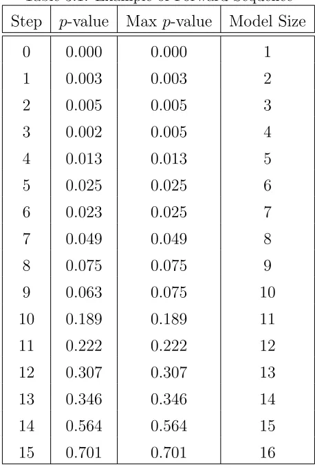
Now that we have a formula for estimating γ, our next goal is to determine a grid of possible choices for α. For any particular dataset, the model size, and therefore false selection rate, only changes at certain values of α. These values correspond to the p-values of the variable being included at a given step of the selection process. While obtaining the forward sequence, we can keep track of the p-values to enter at each step. In particular, the maximum p-value of the current and previous steps is of interest. This list of maximum p-values can be used as the possible estimates for α.

For example, suppose that Table 3.1 gives the 15 steps of a forward selection

(49)

Table 3.1: Example of Forward Sequence

Step p-value Max p-value Model Size

0 0.000 0.000 1

1 0.003 0.003 2

2 0.005 0.005 3

3 0.002 0.005 4

4 0.013 0.013 5

5 0.025 0.025 6

6 0.023 0.025 7

7 0.049 0.049 8

8 0.075 0.075 9

9 0.063 0.075 10

10 0.189 0.189 11

11 0.222 0.222 12

12 0.307 0.307 13

13 0.346 0.346 14

14 0.564 0.564 15

15 0.701 0.701 16

0.005. Once α gets to 0.005, the model size jumps from 2 to 4. An easy way to see the grid and resulting model sizes is by plotting 1 +S(α) by α. Figure 3.1 gives this plot for the example data in Table 3.1. From the plot we can see that in order to obtain

the model sizes, {1, 2, 4, 5, 7, 8, 10, 11, 12, 13, 14, 15, 16}, the minimum values of

(50)

0.0 0.1 0.2 0.3 0.4 0.5 0.6 0.7

5

10

15

α

Model Size

Figure 3.1: Example of step function for model size by α. • indicates the closed lower bound for α corresponding to a specific model size. ◦ indicates the open upper bound forα

corresponding to specific model size.

3.1.2 Choosing Alpha

Once we have our grid of choices for α, we can plug these values into (3.7). Rather than choosing the value which yields ˆγf ast(α) closest to γ0, we choose the largest α

such that ˆγf ast(α)≤γ0. The reasoning is that by choosing the largest model meeting

our false selection goal, a larger proportion of the informative variables are included.

When α = 0, no variables are entered into the model leading to ˆγf ast = 0. But also

when S(α) = Kt, ˆγf ast = 0 as well. These are the cases of fitting a null model and

a full model respectively. Of course we do not believe that the false selection rate of

(51)

process. Therefore, constraints must be added when choosingαto avoid fitting the full model every time. Since ˆγf ast starts and ends at 0 and is nonnegative, there must be a

maximum. Call theαentry-level corresponding to this maximumαmax. Beyond it, the

false selection rates tend to be underestimated with the extreme case being ˆγf ast = 0

for the full model. Therefore, the necessary constraint is to limit our choice of α to those which do not exceed this point. This leads to the estimate,

ˆ

α= sup

α≤αmax

{α : ˆγf ast(α)≤γ0}. (3.8)

Although the continuous interval [0,1] is used in (3.8), it is sufficient to search over

α from the discrete grid. Choosing α from the grid yields an expected false selection rate less than γ0, but results in the same model as choosing over the interval [0,1]. In

general, if αd is the value from the discrete grid that solves (3.8), then the solution

over [0,1] is

ˆ

α= γ0{1 +S(αd)} Kt−S(αd)

.

Using Kt = 15 for the data in Table 3.1, the grid and corresponding estimates of

false selection rate can be found in Table 3.2. Also, Figure 3.2 gives the corresponding

plot of ˆγf ast(α) by α. Notice that ˆγf ast peaks at 0.0859 when α = 0.189. Using the

discrete grid to solve (3.8), we get ˆα = 0.075, whereas solving (3.8) on [0,1] yields ˆ

(52)

Table 3.2: Example of Alpha Grid

α ˆγf ast(α) S(α)

0.000 0.0000 0 0.003 0.0210 1 0.005 0.0150 3 0.013 0.0286 4 0.025 0.0321 6 0.049 0.0490 7 0.075 0.0450 9

0.189 0.0859 10 0.222 0.0740 11 0.307 0.0708 12 0.346 0.0494 13 0.564 0.0376 14 0.701 0.0000 15

3.2 False Selection Rate for Interactions

When considering higher-order effects, the way we approach uninformative variables

changes somewhat. In Chapter 1, a discussion was given on how different units for

predictors can lead to different results when using a model selection process. It was

then suggested that the original predictors be standardized before creating the derived

variables. This would lead an experimenter to the same X matrix no matter what

units he used for measurement. Given that the original predictors are standardized,

we assume that the hierarchy is maintained. Therefore, if an interaction or quadratic

(53)

0.0 0.1 0.2 0.3 0.4 0.5 0.6 0.7

0.00

0.04

0.08

α

γ

^ fast

(

α

)

Figure 3.2: Example plot of ˆγf ast(α) byα

information, we now develop the Fast FSR formulas for the algorithms from Chapter

1.

3.3 No Hierarchy with Fast FSR

In the no hierarchy approach, the Fast FSR methodology works exactly as previously

described. Each effect is a candidate for entry at the beginning of the forward selection

process. Therefore, the probability of any effect being in the candidate set is 1, and

Fast FSR Methods for Second-Order Linear Regression Models

Abstract

Fast FSR Methods for Second-Order Linear Regression Models

Dedication

Biography

Acknowledgements

Table of Contents

List of Tables

List of Figures

Chapter 1

Modeling Interactions in Regression

Analysis

1.1

Introduction

1.2

Issues with Interactions in Regression

1.3

Subset Selection Methods

1.4

No Hierarchy

1.5

Strong Hierarchy

1.6

Weak Hierarchy

Chapter 2

Other Modeling Techniques

2.1

Regression with Shrinkage

2.1.1

Nonnegative Garrote

2.1.2

Least Absolute Shrinkage and Selection Operator

2.2

Recursive Partitioning

2.2.1

Automatic Interaction Detection

2.2.2

Classification and Regression Trees

2.2.3

Chi Square Automatic Interaction Detection

2.2.4

Other Techniques

2.3

Multivariate Adaptive Regression Splines

Chapter 3

Fast False Selection Rate

3.1

Introduction to Fast False Selection Rate

3.1.1

Calculating Alpha Grid

3.1.2

Choosing Alpha

3.2

False Selection Rate for Interactions

3.3

No Hierarchy with Fast FSR