ABSTRACT
WANG, ANRAN. Exploiting Feature Information in Matrix Completion. (Under the direction of Dr. Hua Zhou.)
Matrix completion aims to recover a large matrix of which only a small fraction of
entries are observed. The problem has sparked intensive research in recent years and is
enjoying an increasingly broad range of applications. An archetypal example is the famous
Netflix movie recommendation challenge, where viewers (rows) only rate a small number
of movies (columns) and the goal is to impute unobserved entries of the entire
viewer-movie rating matrix so to predict the ratings of viewer-movies that viewers have not yet rated.
In many such applications, in addition to the observed matrix entries, abundant feature
information is available. In the Netflix example, viewers’ demographic information such
as gender and education, and the movies’ background information such as genre were
present along with the observed ratings. Intuitively, the matrix completion task should
be greatly facilitated by such feature information.
While spectral regularization provides an efficient way to construct a low-rank model
based on observed entries of the matrix, finding an approach that enables incorporating
feature information becomes challenging.
In this thesis, we study the matrix completion problem incorporating feature
infor-mation. In the first part of this thesis, we propose a novel general regularization solution
that simultaneously exploits both the low-rank matrix structure and the rich feature
information. Our solution integrates two types of regularizations, spectral and graph
Laplacian regularizations, and can be viewed as a matrix version of the popular
elas-tic net regularization. We develop highly efficient computational algorithms that have
part, we propose a spectral regularized regression model that can be deemed as a
soft-thresholding of the regression-based latent factor models. Further, we extend the linear
model to the case of logistic regression model for handling binary matrices. Simulations
and real data analyses demonstrate the superior performance of the proposed methods
©Copyright 2015 by Anran Wang
Exploiting Feature Information in Matrix Completion
by Anran Wang
A dissertation submitted to the Graduate Faculty of North Carolina State University
in partial fulfillment of the requirements for the Degree of
Doctor of Philosophy
Statistics
Raleigh, North Carolina
2015
APPROVED BY:
Dr. Lexin Li Dr. Brian Reich
Dr. Zhilin Li Dr. Hua Zhou
DEDICATION
BIOGRAPHY
The author earned her Bachelor of Economics degree from Zhejiang University in 2008.
She received her Master of Financial Mathematics degree in 2010 from North Carolina
State University. Then she joined the doctoral program in Statistics at North Carolina
State University and studied statistical computing in Dr. Hua Zhou’s group. While
pur-suing her doctoral degree, she was also a recipient of the Oak Ridge Institute for Science
and Education fellowship and participated in research projects at US EPA, and worked
ACKNOWLEDGEMENTS
During my years at North Carolina State University, I was fortunate to have Dr. Hua
Zhou as my advisor. Everything that I learned about research was from Dr. Zhou. I have
benefited from meetings with Dr. Zhou since I joined his research group. I appreciate all
his contributions of inspirational ideas, unique experiences in the state-of-the-art
com-puting methodologies, and patient guidance over the years. His enthusiasm in research
motivated me to move forward during tough times. He has always encouraged me to
present projects at meetings and put endless efforts helping me revise the slides. I am
grateful and honored to have the opportunity to work under his direction.
I am also very grateful for the help from Dr. Lexin Li. He provided me advice and
valuable inputs through the research. I would like to acknowledge the other two members
of my defense committee, Dr. Brian Reich and Dr. Zhilin Li for their time, interest and
insightful suggestions.
I also appreciate the assistance on the high performance computing by Dr. Gary
Howell from the Office of Information Technology. And I gratefully acknowledge the
funding sources from US EPA and GlaxoSmithKline that made my Ph.D. study possible.
Most importantly, I would like to thank my beloved family. Thank you for your love
and support. Many friends and groups also became a part of my life here at North
Carolina State University. I am grateful for many people and memories during the seven
CONTENTS
List of Tables . . . vii
List of Figures . . . viii
List of Algorithms . . . ix
Chapter 1 Introduction . . . 1
1.1 Motivation . . . 2
1.2 Thesis Contributions . . . 5
1.3 Notation and Terminology . . . 6
1.4 Outline . . . 8
Chapter 2 Related Work and Background. . . 9
2.1 Spectral Regularization . . . 9
2.1.1 Model Assumption and Fundamentals . . . 11
2.1.2 Nuclear Norm Minimization . . . 13
2.1.3 Minimum Rank Approximation . . . 16
2.2 Graph Laplacian Regularization . . . 17
2.3 Latent Factor Models . . . 20
2.4 Background on Optimization Algorithms . . . 21
2.4.1 Gradient Descent Method . . . 22
2.4.2 Conjugate Gradient Method . . . 23
2.4.3 Proximal Gradient Method . . . 24
Chapter 3 Spectral and Graph Laplacian Regularization . . . 27
3.1 Model Formulation . . . 27
3.2 Optimization Algorithms . . . 30
3.3 Parameter Tuning . . . 35
3.4 Numerical Examples . . . 36
3.4.1 Evaluation Metrics . . . 37
3.4.2 A Simulation Study . . . 38
3.4.3 MovieLens Data . . . 41
3.4.4 Genotype Imputation for Pedigree Data . . . 47
Chapter 4 Spectral Regularized Regression Model . . . 49
4.1 Model Formulation . . . 50
4.2 Optimization Algorithms . . . 50
Chapter 5 Spectral Regularized Generalized Linear Model . . . 61
5.1 Model Formulation . . . 61
5.2 Optimization Algorithms . . . 63
5.3 Numerical Examples . . . 67
Chapter 6 Conclusion . . . 72
Bibliography . . . 74
Appendix . . . 83
Appendix A Appendix . . . 84
LIST OF TABLES
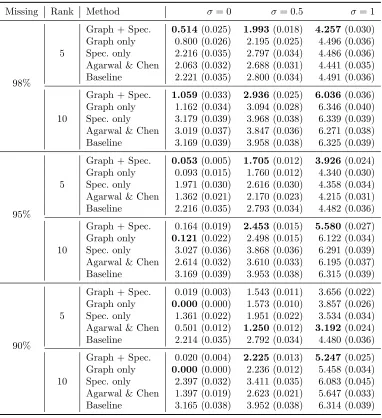
Table 3.1 Averaged RMSE (standard error in parentheses) for methods over 100 simulated data sets under each setting. . . 41 Table 3.2 Performance versus number of grid points for or λn without feature. . 45
Table 3.3 Performance versus number of grid points for or λr and λc at a chosen
λn. . . 45
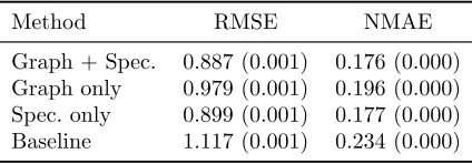
Table 3.4 100K data set: averaged RMSE/NMAE (SD in parentheses) based on 5-fold random partitions of the original data for each of the methods with 80% for training. . . 46 Table 3.5 1M data set: averaged RMSE/NMAE (SD in parentheses) based on
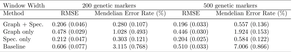
5-fold random partitions of the original data for each of the methods with 80% for training. . . 47 Table 3.6 212 individuals: results averaged over 5 windows (SD in parentheses). 48
Table 4.1 RMSE and standard error (in parentheses) from 100 simulated data sets under each setting. . . 57 Table 4.2 100K dataset: averaged RMSE/NMAE of testing sets (SD in
parenthe-ses) based on 5-fold random partitions of the original data for each of the methods with 80% for training. . . 59 Table 4.3 1M dataset: averaged RMSE/NMAE of testing sets (SD in parentheses)
based on 5-fold random partitions of the original data for each of the methods with 80% for training. . . 60
Table 5.1 NMAE and standard error (in brackets) from 100 simulated data sets under each setting. . . 69 Table 5.2 100K dataset: averaged NMAE of testing sets (SD in parentheses) based
LIST OF FIGURES
Figure 1.1 A sample pedigree (sister-brother mating) with 6 members and the corresponding kinship coefficient matrix Φ capturing the degree of relatedness among them. . . 4
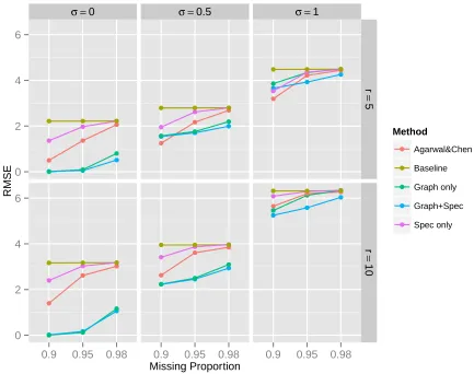
Figure 3.1 Data matrix Y under different levels of within-cluster variation σ. . . 39 Figure 3.2 Averaged RMSE for methods over 100 simulated data sets under each
setting. . . 42 Figure 3.3 Sensitivity on the choice of the regularization parameter λn with 20
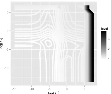
grid points (left pane) and 400 grid points (right pane). . . 44 Figure 3.4 RMSE for different regularization parameters λr and λc with 20 grid
points. . . 44
Figure 4.1 Averaged RMSE for methods over 100 simulated data sets under each setting. . . 58
LIST OF ALGORITHMS
Algorithm 1 Conjugate gradient method . . . 23
Algorithm 2 Line search (Beck and Teboulle, 2009) . . . 25
Algorithm 3 Nesterov method for minimizing (3.2) in spectral and graph
Laplacian regularization method. . . 34
Algorithm 4 Nesterov method for minimizingh(Θ|β,γ) in spectral regular-ized linear regression model. . . 54
Chapter 1
Introduction
This thesis deals with the problem of imputing large and sparse matrices. Motivated by
real world applications, we aim to develop methods for improving on the imputation
per-formance by utilizing the rich additional feature information. How to construct general
regularizations that incorporate the additional feature information, and how to efficiently
compute the solutions are the main topics in this thesis. More importantly, convex
op-timization problem is the foundation of our approaches, which distinguishes our work
from the other existing research in incorporating feature information to the conventional
matrix completion framework. We begin by giving a statement of the matrix completion
problem in Section 1.1, then introduce our contributions in this domain in Section 1.2,
also we provide an overview of the notation and terminology that will be used throughout
1.1
Motivation
Matrix completion concerns recovering or imputing a large matrix of which only a small
fraction of entries are observed. The problem has received considerable attention when
the movie distribution company Netflix offered a million dollar prize for improvement on
its movie rating system (ACM SIGKDD and Netflix, 2007). The Netflix data consisted
of 100,480,507 ratings collected from 480,189 users on 17,770 movies. Netflix would like
to infer the users’ preferences and recommend additional movies for their consideration
based on the ratings they submitted. The data can be phrased in the form of a matrix
whose rows are users and columns are movies. And the elements of the matrix are the
movie ratings assigned by the users. It is noteworthy that this matrix is extremely sparse,
as an individual user only rated a tiny subset of movies compared to the entire database
of Netflix movies. Here almost 99% of the entries in this data matrix are unobserved.
The goal is then to fill the empty entries of the matrix, i.e., to complete the matrix.
This movie rating application is a special instance of a much broader class of
recom-mendation system problems where items, such as movies, news articles, and
advertise-ments, are recommended to suitable users. Matrix completion has proven a particularly
useful technique to address such problems. Moreover, matrix completion has an
increas-ingly wide range of applications far beyond the setting of the recommendation system.
For example, in a network of sensors, estimating all the pairwise distances of the sensors
are interested, when only the distances between close-by sensors are available. Matrix
completion can be used to solve this global-positioning problem based on the partial
ob-served distance matrix (Singer, 2008; Weng, 2009). In the structure-from-motion problem,
many pixels are missed due to tracking failures in a video sequence. The camera motions
Also, filling in missing genotypes in genome scans for disease genes benefits from matrix
completion. Here the matrix to be imputed is indexed by study individuals in rows and
genetic markers in columns. Matrix completion algorithm is an effective genotype
impu-tation tool in genomic studies (Chi et al., 2013). When conventional matrix completion
problems focus on exploiting observed entries of the matrix in these fields, there is a
growing interest in problems that involves additional feature information.
In many applications, in addition to the observed matrix entries, rich feature
infor-mation is available. Here are two concrete examples.
Customer Ratings
In movie rating (e.g. Netflix) or merchandise rating (e.g. Amazon) problems, feature
information may be available on both users and the items being rated. Users’ demographic
information such as gender and education, and the items’ background information such
as genre were present along with the observed ratings. Individuals in the same age group,
with similar education background, and of same gender, in general, are likely to give
similar ratings to similar items. Movies of same genre or from the same director are
likely to receive similar ratings from same people. Intuitively, the matrix completion task
should be greatly facilitated by such feature information.
Genotype imputation for pedigree data
In the genotype imputation problems, most state-of-art imputation methods take the
convenient independence assumption and perform poorly when imputing family data.
This becomes an increasing concern as geneticists are moving toward genome-wide studies
based on pedigrees (Ott et al., 2011). The genetic relatedness between individuals is well
Figure 1.1: A sample pedigree (sister-brother mating) with 6 members and the corre-sponding kinship coefficient matrix Φcapturing the degree of relatedness among them.
are the probability that a gene randomly selected from individualiand a gene randomly selected from the same autosomal locus of individual j are identical by descent. Figure 1.1 displays a sample pedigree with 6 members and the corresponding Φ. The imputed genotypes should be closer for two individuals with larger kinship coefficient. Properly
incorporating this quantitative measure of individual relatedness into matrix completion
algorithm should boost the imputation accuracy for pedigree data.
Intuitively, the matrix completion task should be greatly facilitated by such feature
information. First of all, incorporating the additional feature information can help
im-prove on the prediction accuracy of matrix completion. Further, conventional methods
of matrix completion based on solely the observed entries are not able to deal with the
situation that new users or items join the data matrix and few historical ratings are
pro-vided. Hence, in this case, exploiting the additional feature information from the users
or items to assist prediction becomes necessary. However, extending conventional
feature information is challenging.
1.2
Thesis Contributions
The importance of using the additional feature information from the rows and columns
have not been realized widely in the existing research of matrix completion problems.
Currently, in this emerging field of learning additional feature information, most of
ex-tensions of conventional matrix completion approaches that exploit feature information
(Singh and Gordan, 2008; Ma et al., 2008, 2011a; Zhen et al., 2009; Agarwal and Chen,
2009) are based on matrix factorization techniques, which result in non-convex
optimiza-tion problems. Hence, these approaches face the difficulty to optimize globally and lack
of theoretical guarantee of perfectly recovering target matrices.
In this thesis, we propose two approaches under the framework of convex
optimiza-tion problems to incorporate feature informaoptimiza-tion in aiding matrix compleoptimiza-tion. Our first
approach is a general regularization solution via spectral regularization and graph
Lapla-cian regularization. A spectral regularization is implemented employing the nuclear norm,
which is a suitable convex relaxation of the rank constraint (Recht et al., 2010), and in
effect induces a low-rank structure on the reconstructed matrix. Meanwhile, a graph
Laplacian regularization drawn from other research areas is coupled with the spectral
regularization, which effectively integrates the low-rank structure with correlations
be-tween imputed entries that are indicated by feature information. This new joint
regu-larization framework can be deemed as a matrix version of the popular elastic net (Zou
and Hastie, 2005) regularization for vector parameters. This approach shows superior
performance in predicting user preferences on items compared to conventional matrix
in-formation in genotype imputation. The second approach is an integration of spectral
regularization and regression models, which can be cast as a soft-thresholding version of
regression-based latent factor models (Agarwal and Chen, 2009), and more importantly,
it avoids the associated hassles of non-convex optimization. We also extended the linear
model to the case of logistic model for dealing with binary matrices.
In addition, algorithms in our approaches are easy to parallelize. We exploit parallel
computing for reducing the time complexity. In contrast, there are few existing research
studies on parallel matrix completion.
1.3
Notation and Terminology
Scalar and Vectors
For a scalar x, x+ = max(0, x). We denote the set of n-dimensional real vectors by Rn.
For a vector x∈ Rn, we usex
i to indicate the i-th element of the vector. And we write
card(x) for the cardinality, which is the number of elements in a vectorx. The l1-norm of
a vectorxis defined askxk1 =Pni=1|xi|, and thel2-norm is defined askxk2 =pPni=1x2i.
The inner product of x andy is denoted by hx, yi. We use ∇f(x) to denote the gradient of f(x), which is defined by ∇f(x) = (∂f∂x(x)
1 , ∂f(x)
∂x2 , . . . , ∂f(x)
∂xn ) T.
Matrices
We denote the space of real m byn matrices by Rm×n. For a matrix X ∈Rm×n, we use
xij to denote the entry in the i-th row andj-th column, Xi· the i-th row of the matrix, and X·j the j-th column of the matrix. The rank of (X) is denoted by rank(X). We use
XT for the transpose of X, and Tr(X) for the trace of X. Define 1/X as elementwise
off(X) is denoted by∇f(X). For two matricesX ∈Rm×n andY ∈
Rp×q, the Kronecker
product, denoted byX ⊗Y, is defined as
X⊗Y =
x11Y · · · x1nY
..
. . .. ...
xm1Y · · · xmnY
,
amp×nq block matrix. The entrywise product is denoted by X∗Y. We usehX,Yito denote the inner product of corresponding column stacked vectors of X and Y. Let In
denote a n×n identity matrix.
Singular Value Decomposition (SVD)
A rank-r matrix X ∈ Rm×n can be expressed in the SVD form, X = UΣVT, where
Σ = diag({σi(X)}1≤i≤r), σi(X) is the i-th singular value of X sorted in descending
order, and U ∈Rm×r and V ∈
Rn×r are matrices with orthogonal columns.
Nuclear Norm
Let kXk∗ denote the nuclear norm (or trace norm) of a matrix X ∈Rm×n with rank r.
It is defined as the sum of its singular values,
kXk∗ =
r
X
k=1
σk(X),
where σk(X) is thek-th singular value of the matrixX sorted in decreasing order.
Frobenius Norm
kXkF =
p
hX,Xi= v u u t
r
X
k=1
σ2
k(X).
1.4
Outline
The rest of the thesis is organized as follows. Chapter 2 reviews three lines of research
related to our work and describes the background of optimization algorithms. In
Chap-ter 3, we formulate a novel general regularization framework via spectral regularization
and graph Laplacian regularization for matrix completion involving additional feature
information, and develop computational algorithms to solve the optimization problems.
We also investigate the performance on simulated and real-world data examples. Chapter
4 proposes a spectral regularized regression model. We describe the model formulation,
derive optimization algorithms and demonstrate the numerical performance. In Chapter
5, we extend the linear model proposed in Chapter 4 to the case of logistic model for
dealing with binary matrices. In Chapter 6, we conclude the thesis with a discussion of
Chapter 2
Related Work and Background
In this chapter, we review research studies that are related to our work including the
conventional matrix completion techniques and the emerging field with additional feature
information. Our proposed approaches are related to but also distinctive from three lines
of recent development concerning regularizations. In Section 2.1-2.3, we recall the key
developments in these three lines of regularizations. Then we introduce the background
on algorithms of various optimization problems related to our work in Section 2.4.
2.1
Spectral Regularization
The first is a body of work on various aspects of conventional matrix completion that
focus solely on the observed entries of the matrix. Extensive methods have been
devel-oped to address the problem including nuclear norm regularization (Srebro, 2004; Srebro
et al., 2004b), efficient computational algorithms (Mazumder et al., 2010; Cai et al.,
2010; Recht, 2011), generalization error bounds (Srebro et al., 2004a), prediction error
Cand`es and Tao, 2010; Keshavan et al., 2009b), completion from noisy entries (Keshavan
et al., 2009a; Negahban and Wainwright, 2010), and weighted nuclear norms
(Salakhut-dinov and Srebro, 2010). These research studies, in particular the low-rank type matrix
completion methods for the recommender systems can be generalized to spectral
regu-larization (Abernethy et al., 2009) as follows, which makes algorithms robust to noise in
the data.
Suppose user profiles are elements in a Hilbert space X, the item profiles are the
elements of another Hilbert space Y, and the ratings of users for items are the elements
in R. Inferring a function f : X × Y →R can be used to predict the rating of any user
x ∈ X for any item y ∈ Y. Consider a linear preference function f(x, y) = hx, F yiX for some compact operator F that maps from X to Y. Spectral regularization can be described as a function Υ that only depends on the singular values of F,
Υ(F) =
d
X
i=1
si(σi(F)),
where si is a non-decreasing penalty function with si(0) = 0, and {σi(F)i=1,...,d} are the
dsingular values of F in decreasing order. A class of spectral penalty functions including the following cases are used commonly in conventional matrix completion problems.
Rank Regularization
Given r, if si(x) = 0 for i = 1, . . . , r, sr+1(x) = 0 for x = 0, and sr+1(x) = +∞ for
Nuclear Norm Regularization
If si(x) =x for all i, then it forms the nuclear norm penalty,
Υ(F) =
d
X
i=1
σi(F) = kFk∗.
Frobenius Norm Regularization
If si(x) =x2 for all i, then it forms the squared Frobenius norm penalty,
Υ(F) =
d
X
i=1
σi2(F) =kFk2
F.
In the matrix completion problems, sparsity is a key issue. For instance, in the Netflix
Prize data, only approximately 1% entries of the matrix are observed, and it can raise
the over-fitting problem. Adding spectral regularization can control the impact of noise
and prevent over-fitting. Among various classes of spectral regularization, the nuclear
norm regularization and the rank regularization to obtain a low-rank structure in the
solution have attracted considerable research attention in conventional matrix completion
problems. In the following sections, we review optimization problems with these two
special cases of spectral regularization.
2.1.1
Model Assumption and Fundamentals
In general, it is theoretically impossible to determine the missing entries of a matrix
based on only a small number of observed entries. However, with certain assumptions
on the structure of the matrix, it is possible to reconstruct matrices via various
similar ratings on the same items tend to have similar preferences. Assuming the
rat-ings observed are collaborations induced by characteristics from users and items, we can
impute the ratings jointly for users and items. Intuitively, the ratings depend on only a
few characteristics, that is, only a small number of characteristics of the users and the
items contribute to preferences of users on items. This number should be much less than
the number of users and the number of items. In this context, modeling the matrix with
the low-rank structure is an appealing strategy to capture hidden structures of the data
matrix.
We now describe two scenarios, the observed entries without noise and another
sce-nario with noise. Denote the unknown matrix to be completed by Y ∈Rm×n, where m is the number of users, and n the number of items. The (i, j)th entry of Y is the rating
that user i would assign to the item j. Let ∆ denote the set of the indices of observed entries or ratings, and letX ∈Rm×n denote the estimator of Y or the decision variable matrix. LetP∆ denote the sample operator that its element
[P∆(X)]ij =
xij, (i, j)∈∆,
0, otherwise.
When there is no noise, the matrix completion problem aims to recover Y from the
observed entries in ∆, and a constraint P∆(X) = P∆(Y) can be assumed. However,
in many real-world applications, such as in the recommender systems, the entries would
contain errors and noise. To be more general, matrix completion problem can be modeled
by assuming partial information about the target matrix is received, that is, P∆(Y) +
P∆(Z), which is the sum of an unknown low-rank matrix Y and an unknown noise or
Y from the observed partial information. Based on convex optimization of the nuclear
norm, realization possibilities and theoretical guarantee of matrix completion have been
established. For the scenario without noise, it has been proved that assuming there is
an unknown low-rank matrix, if the number of observed entries is sufficiently large and
under certain conditions on the entries of the matrix and locations, then the target matrix
can be completed exactly with a high probability (Cand`es and Recht, 2009; Cand`es and
Tao, 2010; Recht, 2011; Gross, 2011; Keshavan et al., 2010). When noise exists, also it
has been shown that it is possible to approximately reconstruct the unknown low-rank
matrix from observed entries, if the matrix satisfies appropriate conditions (Cand`es and
Plan, 2010; Negahban and Wainwright, 2010). This thesis does not go in depth into the
theoretical guarantee and fundamental limits. Extensive research covers the paradigm for
convex problems in matrix completion techniques.
2.1.2
Nuclear Norm Minimization
To capture the assumptions, one can impute the matrix by adding constraints on the
possible matrices. The common low-rank assumption of the matrix leads to a constrained
matrix rank minimization problem. If the number of the observed entries is sufficiently
large, under the noiseless scenario, the problem is to find a low-rank matrix that matches
the observed entries. The matrix rank minimization problem can be formulated as
minimize rank(X)
subject to P∆(X) = P∆(Y).
(2.1)
The idea is to find a low-rank matrix that fits the observed entries. However, the rank(X)
known to be computationally intractable hard (NP-hard) (Chistov and Grigoriev, 1984).
Approximation formulations have been introduced for the practical applications.
To be computationally tractable, breakthrough papers (Fazel et al., 2001; Cand`es and
Recht, 2009; Cand`es and Tao, 2010; Recht et al., 2010) showed that the nuclear norm
is the tightest convex relaxation of the non-convex function rank(X). In the research
papers (Cand`es and Tao, 2010; Cand`es and Recht, 2009; Cai et al., 2010), the nuclear
norm minimization was used as a convex surrogate to approximate the original rank
minimization problem (2.1). The formulation of the problem is given by
minimize kXk∗
subject to P∆(X) = P∆(Y).
The problem was then generalized to the scenario with noise by relaxing the constraint
(Cand`es and Plan, 2010),
minimize kXk∗
subject to kP∆(X)− P∆(Y)kF ≤δ,
(2.2)
whereδ > 0 is the regularization parameter that controls the tolerance in training error. Based on (2.2), the nuclear norm minimization problem can be reformulated in an
equiv-alent Lagrange form (Cai et al., 2010). It penalizes the training error or the aggregate
loss over observed ratings by the squared Frobenius norm,
minimize 1
2kP∆(Y)− P∆(X)k
2
F +λkXk∗. (2.3)
based on a general version of the nuclear norm regularized convex optimization problems
over matrices,
minimize f(X) +λkXk∗,
where f(X) is a differential convex loss function. It is a generalization of the l1-norm
regularized problem for vectors to the case of matrices.
Nuclear Norm Based Algorithms
Extensive nuclear norm based algorithms have been developed for solving the matrix
completion problems. A number of researchers have studied variations of spectral
regu-larization in formulation with a variety of penalization functions, such as power family
and SCAD (Zhou and Li, 2012). On the other hand, a difficulty with the nuclear norm
minimization is that, kXk∗ is not differentiable. For solving the nuclear norm
minimiza-tion problem, there are many efficient algorithms that consider certain variaminimiza-tional forms
of the singular value decomposition (SVD) as computational solvers. SVD is a
dimension-ality reduction technique. These algorithms do not pre-specify the rank of the matrix,
and optimize the penalized nuclear norm problem iteratively, such as the singular value
thresholding (SVT) (Cai et al., 2010), the soft-impute (Mazumder et al., 2010), the fixed
point continuation with approximate SVD (Ma et al., 2011b), and the accelerated
prox-imal gradient (Toh and Yun, 2010). These algorithms can be easily trained to achieve
both good accuracy and efficiency.
Take the SVT algorithm for example, it is one of the efficient and commonly used
al-gorithms that aims to solve (2.3). The SVT involves SVD and applies a soft-thresholding
operator on the singular values at each iteration (Cai et al., 2010). The nuclear norm
regulariza-tion or thresholding parameter λ. This algorithm uses the linearized Bregman iteration. It computes SVD, then retains the singular values larger thanλto form a truncated SVD at each step using a shrinkage operator.
2.1.3
Minimum Rank Approximation
Some researchers solve the matrix completion problems by estimating a low-rank matrix
X which minimizes the distance between X and Y at the observed entries, with a
constraint that the rank ofX is less than or equal to a constant value. The problem can
be cast as
minimize kP∆(X)− P∆(Y)kF
subject to rank(X)≤r.
(2.4)
Any matrix X ∈ Rm×n with rank r at most can be expressed as X = U VT, where
U ∈ Rm×r and V ∈
Rn×r. To improve on the problem (2.4), the matrix factorization
techniques have been introduced by research papers (Srebro and Jaakkola, 2003; Rennie
and Srebro, 2005; Srebro et al., 2005) which factorize the decision matrixX and minimize
over U and V alternatively. The modified objective function is given by
min
U∈Rm×r
min
V∈Rn×r
1
2kP∆(U V
T)− P
∆(Y)k2F +
λ
2(kUk
2
F +kVk
2
F).
With this modification, the rankrcan be adjusted. Later, matrix factorization techniques with the most common formulation below have attracted considerable attention (Koren
et al., 2009),
min
U∈Rm×r
min
V∈Rn×r
1
2kP∆(U V
T)− P
∆(Y)k2F +
λu
2 kUk
2
F +
λv
2 kVk
2
where λu and λv are the regularization parameters. This version has advantages with
respect to scalability and accuracy. The task of matrix factorization techniques is to
estimate the low-rank representations or latent factors of users and items based on the
observed entries of the matrix. Here U and V can be deemed as two matrices of latent
factors. Matrix factorization can be formulated as a probabilistic model (Salakhutdinov
and Mnih, 2008b,a) that models the conditional probabilities of latent factors given the
observed entries.
Since algorithms for the matrix factorization do not require SVD, they are
com-putational cheaper than the nuclear norm minimization algorithms. However, the key
drawback of the matrix factorization approaches is the non-convexity. Algorithms for
solving this problem can be easily trapped in a local minimum and fail to converge to
the global minimum. Hence even though the matrix factorization techniques may have
good performance on some recommender system examples, results can be inconsistent
when algorithms converge to different local minima, and they are unable to explore the
whole low-rank space (Xin, 2012).
To prevent this issue, our work uses convex spectral penalty functions, that is, a
nuclear norm based optimization problem. The key difference of our work and the
con-ventional nuclear norm minimization method is that we utilize feature information along
with matrix reconstruction, whereas existing methods mainly focus on observed matrix
entries.
2.2
Graph Laplacian Regularization
Spectral regularization approaches represent the largest body of work in conventional
grow-ing with increasgrow-ing availability of feature information. This line of work involves various
forms of graph Laplacian regularization, including network constrained variable
selec-tion (Li and Li, 2008, 2010), random walk smoothing (Zhou et al., 2005a,b), Tikhonov
regularization with undirected graph (Belkin et al., 2004), manifold regularization with
undirected graph (Belkin et al., 2006; Wu et al., 2010). First we recall the concept of the
graph Laplacian.
Graph Laplacian Matrix
The Laplacian matrixLof a simple graphGrepresents the graph in a matrix form, where
Gis undirected, unweighted without graph loops and each edge of G is a pair of distinct vertices. The relations between pairs of vertices of an undirected graph are symmetric.
The graph G consists of a set of vertices V and a set of edges E, where pairs (i, j) ∈E
and i, j ∈V. The Laplacian matrix is an n×n symmetric matrix, if G has n vertices. It is defined as
L=D−K,
whereD= diag({P
jkij}1≤i≤n) is the degree matrix ofK, andK is the adjacency matrix
of G. The value of kij is the number of edges from vertex i to j. When it is extended
to weighted graphs, kij can be a weight associated with each edge (i, j). It measures the
differences of values at a vertex from nearby vertices of the graph.
Regularization
The graph Laplacian can be used in designing regularization operators by penalizing the
differences between adjacent vertices. It has been shown that learning on graphs can be
y on a graph with the weighted matrix K (Zhou et al., 2005a; Belkin et al., 2006; Wu et al., 2010),
minimize X
i,j
kij(fi−fj)2+
λ
2kf−yk
2 2,
where λ > 0 is the regularization parameter. The first term measures the smoothness of the function f, and the second term penalizes its distance to y. It has been shown that P
i,jkij(fi−fj)2 =fTLf. Tikhonov regularization (Belkin et al., 2004) finds f by
solving this problem,
minimize kf −yk22+λfTLf.
Graph based approaches have also been studied in the field of link prediction in
social networks (Liben-Nowell and Kleinberg, 2003; Gori and Pucci, 2007; Jamali and
Ester, 2009). The algorithms based on graphs summarize information in one graph and
then apply a graph mining technique. The graph consists of user nodes, item nodes and
nodes representing other entities. The relationship between a user and an item could be
weighted by a rating, whereas the relationship between two users could be weighted by
the friendship. Graph-based approaches have also been applied on investigating the effect
of social tagging on different ranking tasks (Clements et al., 2010) and social relationship
(Bu et al., 2010).
These approaches aim at correlated data on a graph or network in a regression
(su-pervised) setting, and the regression parameters involved take the form of vectors. By
contrast, our work deals with parameters in matrix forms, and the graph Laplacian
reg-ularization is utilized to capture entry correlations induced by feature information of the
2.3
Latent Factor Models
In recent years, the emerging additional feature information beyond the observed matrix
has started to form the new scenarios of matrix completion. The third family employs
latent factor models to build personalized recommendation systems (Hofmann, 1999;
Banerjee et al., 2007; Agarwal and Merugu, 2007; Agarwal and Chen, 2009; Agarwal
et al., 2011). In this line of work, they apply the assumption that ratings are influenced
by certain hidden factors. These factors are not obvious and their impact on the ratings
might be difficult to estimate. Their goal is to infer these so called latent or hidden factors
from the data. The algorithms in this line of work extend the matrix factorization
tech-niques, one of the conventional matrix completion approaches we introduced in Section
2.1.3, to a general version that incorporates feature information from users and items in
addition to the observed entries of the matrix.
Begun with collective matrix factorization method (Singh and Gordan, 2008), matrix
factorization techniques have drawn attention. This approach is also referred to as joint
matrix factorization. It simultaneously factorizes multiple related matrices, including
the observed matrix and matrices containing the feature information. Model parameters
include latent factors of users, items, the user feature information entity and the item
feature information entity. These latent factors are inferred based on the observed entries
of the matrix and the relation matrices of users or items and their feature information
entity. Collective matrix factorization has also been applied to research on social networks
(Ma et al., 2008, 2011a) and tags (Zhen et al., 2009). The probabilistic interpretation
of the collective matrix factorization method (Porteous et al., 2010) was proposed to
model the conditional probabilities of the latent factors of users and items with feature
Among other latent factor models, one of the most influential approach is the
regression-based latent factor models (Agarwal and Chen, 2009). It proposed to integrate feature
information of both users and items with the observed entries of the matrix into a
gen-eralized linear model for preference prediction. This work developed regression models
to utilize users and items features, and partly thanks to such utilization, their approach
represents the state-of-the-art solution to recommendation.
However, their method and our work differ in several ways. Latent factor models fix
the rank of the matrix decomposition, and can be viewed as a hard-thresholding type of
regularization. By contrast, our method imposes the nuclear norm to induce a low-rank
structure and is a soft-thresholding regularization. Since the these methods introduced
in this section consider the matrix factorization techniques as their foundation, they still
encounter the non-convex optimization problems. Moreover, Bayesian formulations are
commonly adopted in latent factor modeling, which produces a considerable number of
tuning parameters. Our approaches instead hinge on only one to three tuning
param-eters, and thus are much simpler to tune. Finally it is unclear how genetic relatedness
information, as the genotype imputation example indicates, is to be incorporated with
regression based latent factor models.
2.4
Background on Optimization Algorithms
In this section, we introduce a variety of iterative optimization algorithms that will be
used throughout the thesis to find the minimum of convex objective functions. When
the minimum of a function can not be found analytically or direct methods may take
too much time, iterative optimization methods can be used to obtain an approximate
2.4.1
Gradient Descent Method
To minimize a convex function f(x), one strategy is to employ line search methods (Nocedal and Wright, 2006), which are a family of iterative optimization methods. Each
iteration of a line search method is given by
x(k+1) =x(k)+δ(k)p(k),
where δ(k) >0 is the step size andp(k) is the search direction. The idea is to move along a direction or a line and compute how far the previous search point x(k) should move, so that f(x(k+1))< f(x(k)). The procedure for choosing the step size in the search direction
is called a line search method. The step size can be determined exactly by minimizing
f∗(δ) =f(x(k)+δp(k)) over δ, or loosely by requiring a sufficient decrease in f∗.
One of the basic line search methods is the gradient descent method (Arfken, 1985).
For a differentiable convex functionf(x), the gradient descent method takes steps in the direction of a descent gradient. This method starts with an initial guess pointx(0) for the minimum, then computes a sequence of iterates,
x(k+1) =x(k)−δ(k)∇f(x(k)).
2.4.2
Conjugate Gradient Method
Suppose we aim at solving linear systems of equations Ax=b, instead of using a direct solver, this problem can be cast as minimizing a quadratic functionf(x) = 12xTAx−bTx. Here A∈Rn×n is a symmetric positive definite matrix, i.e., xTAx ≥0, for all non-zero
x, andb ∈Rn is a given vector. Since the gradient off isAx−b, the solution of the linear system and the minimizer off are equivalent. The conjugate gradient method (Hestenes et al., 1952) can be used to handle sparse and large matrices A’s that are too large for
direct methods such as the Cholesky decomposition. The algorithm is given as follows.
1 Initial x(0), r(0) =Ax(0)−b, p(0) =−r(0); repeat 2 δ(k)= (r
(k))Tr(k)
(p(k))TAp(k);
3 x(k+1) =x(k)+δ(k)p(k); 4 r(k+1)=r(k)+δ(k)Ap(k); 5 β(k) = −(r
(k+1))Tr(k+1)
(r(k))Tr(k) ;
6 p(k+1) =−r(k+1)+β(k)p(k);
7 until objective value converges;
Algorithm 1: Conjugate gradient method
where p(k) is a direction vector, and the set of directions {p(i)}
0≤i≤k is a set of mutually
conjugate directions with respect to A, i.e. (p(i))TAp(j) = 0 for all i 6= j. Since such
vectors in this set are linearly independent, this set is a basis of Rn. The solution can be expanded within this set. And r(k) = Ax(k) −b is referred to as the residual vector.
2.4.3
Proximal Gradient Method
A key optimization issue for the nuclear norm based approaches is that though kXk∗ is
convex, it is not differentiable. In order to optimize convex non-smooth functions, one
strategy is to use the proximal gradient method (Martinet, 1970; Bruck Jr., 1977). For a
problem with a target functionh that splits into two components,
minimize h(x) =f(x) +l(x) (2.5)
where function f is convex and differentiable, and functionl is convex and possibly non-differentiable. Using proximal gradient method to solve this problem is inexpensive. The
proximal operator of a convex function J is defined as
proxJ(x) = argmin
u
J(u) + 1
2ku−xk
2 2
.
For the case thatJ(X) = kXk∗, if the SVD ofX =Pdiag({σi}1≤i≤n)QT, then proxλJ(X) =
Pdiag({σˆi1≤i≤n})QT. Here thresholding to singular values σi is applied,
ˆ σ =
σi−λ σi > λ
0 |σi| ≤λ.
σi+λ σi <−λ
The proximal gradient iteration for solving (2.5) is given by
x(k+1) = proxδ(k)l x(k)−δ(k)∇f(x(k))
= argmin
x
l(x) + 1
2δ(k)kx−(x
(k)−δ(k)∇f(x(k)))k2
F
Here ∇f is Lipschitz continuous with constant L(f) > 0, i.e., k∇f(x)− ∇f(y)k2 ≤
L(f)kx−yk2, for allx, y. Typically a fixed step sizeδ(k) ∈(0,1/L(f)] is used. IfL(f) is not
known, the step size can be determined by a line search (Algorithm 2). An interpretation
of the solution (Beck and Teboulle, 2010) is trading off minimizing l and being close to the standard gradient step x(k)−δ(k)∇f(x(k)), determined by δ(k). Then consider a
convex upper bound of f,
ˆ
f(x|x(k)) =f(x(k)) +∇f(x(k))T(x−x(k)) + 1
2δ(k)kx−x (k)k2
2,
satisfying ˆf(x|x(k)) ≥f(x), and ˆf(x|x) = f(x), when δ ∈(0,1/L(f)]. A surrogate
func-tion ofhisg(x|x(k)) = ˆf(x|x(k)) +l(x). Herexminimizesl plus a quadratic local model of
f around x(k). The solution x(k+1) = argmin
x
g(x|x(k)) can be shown equivalent to (2.6).
1 given x(k), δ=δ(k−1), line search parameter α∈(0,1).repeat 2 xtemp = proxδl(x(k)−δ∇f(x(k)));
3 break if f(xtemp)≤fˆ(xtemp|x(k));
4 δ =αδ;
5 return x(k+1) ←xtemp, δ(k) ←δ;
Algorithm 2: Line search (Beck and Teboulle, 2009)
The accelerated proximal gradient method (Nesterov, 1983), known as an accelerated
version of the proximal gradient method with an extrapolation step in the algorithm,
In each iteration, two steps are performed as follows.
1. s(k+1) =x(k)+β(k)(x(k)−x(k−1));
2. x(k+1) = proxδ(k)l s(k+1)−δ(k)∇f(s(k+1))
;
where βk ∈ [0,1) is an extrapolation parameter. In the step of extrapolation, we obtain
an search point based on the previous two iterations. The second step applies the
prox-imal gradient method to this search point. Analogous algorithms have been developed
(Nesterov, 2005, 2007; Tseng, 2008; Beck and Teboulle, 2009) using different step sizes
Chapter 3
Spectral and Graph Laplacian
Regularization
In this chapter, we propose a general regularization solution that simultaneously exploits
both the low-rank matrix structure and the additional feature information. Our approach
integrates two types of regularizations, spectral and graph Laplacian regularizations, and
can be viewed as a matrix version of the popular elastic net regularization. We begin with
model formulation in Section 3.1, describe the optimization algorithms and parameter
tuning in Section 3.2-3.3, and numerical samples are given in Section 3.4.
3.1
Model Formulation
We first briefly review the nuclear norm regularization for matrix completion (Mazumder
et al., 2010) and then detail how feature information can be encapsulated by graph
Spectral Regularization for Matrix Completion
Let Y = (yij) ∈ Rm×n be the matrix to be completed. Let ∆ denote the set of index
pairs (i, j) such that yij is observed, and wij = 1{(i,j)∈∆} be the indicator whether the (i, j)-entry is observed. The spectral regularization proposed (Mazumder et al., 2010) minimizes the criterion
1 2
X
(i,j)∈∆
(yij −xij)2 +λkXk∗ = 1 2
X
i,j
wij(yij−xij)2+λ
X
k
σk (3.1)
with respect to a compatible matrixX = (xij) with singular valuesσk. The nuclear norm kXk∗ =Pkσk plays the same role in low-rank matrix approximation that the `1 norm
kbk1 =
P
k|bk| plays in sparse regression. In some applications such as the genotype
imputation, wij may take general nonnegative values (Chi et al., 2013).
Incorporating Feature Information via Graph Laplacian
Feature information zi ∈ Rp along the rows, when available, can be effectively
sum-marized by a similarity function kij = K(zi,zj). We assume K ∈ Rn×n is symmetric
with nonnegative entries. Most commonly used kernel functions (Scholkopf and Smola,
2001), such as the Gaussian kernel, polynomial kernel, and the Markov chain-based
ker-nels (Zhu et al., 2012) constitute convenient choices for the pairwise similarity measure
based on feature information. However, positive semi-definiteness of K is not required.
In the genotype imputation problem, the kinship coefficient matrix Φ such as displayed in Figure 1.1 is a natural choice for K. The similarity matrix K = (kij) can be viewed
as an adjacency matrix of a weighted graph, where the weightskij capture the closeness
between the i-th and j-th rows. Correspondingly we define the degree matrix D to be the diagonal matrix such that Dii =
P
is defined as L=D−K. For anyx, we have
xT
Lx=X
i
X
j
kijx2i −
X
i
X
j
kijxixj =
1 2
X
i,j
kij(xi−xj)2 =
X
(i,j):i6=j
kij(xi−xj)2,
where the last sum is over n2 pairs. Since x is arbitrary, it immediately follows that
the Laplacian matrixL is positive semidefinite wheneverkij ≥0 for all i, j. Moreover, it
naturally suggests the graph Laplacian as a regularizer to push the neighboring entries
on graph closer. Similarly, when feature information along the columns is available, we
denote the corresponding column space graph Laplacian matrix byH.
To incorporate both the low-rank structure and additional feature information, we
propose to minimize the convex function
h(X) = 1 2
X
i,j
wij(yij −xij)2+
λr
2mtr(X
T
LX) + λc
2ntr(XHX
T
) + λn
q kXk∗
= 1 2kW
1/2∗(Y −X)k2 F+
λr
2mtr(X
T
LX) + λc
2ntr(XHX
T
) + λn
q kXk∗,
(3.2)
where the matrix W1/2 = (w1/2
ij ), ∗ denotes the Hadamard (elementwise) matrix
multi-plication,q= min{m, n}, andλr, λc, λn≥0 are tuning constants. The first regularization
term enforces the predictions at rows that are close in the feature space similar. And the
second regularization term enforces the predictions similar, if columns are close in the
feature space. The appended nuclear norm regularizer promotes a low-rank structure in
the solution.
Special Cases
The regularization framework (3.2) can be considered as a matrix version of the popular
Intuitively, we find a low-rank prediction matrix X that approximates the observed
entries well subject to graph Laplacian regularizations in its row and column spaces.
When λr = λc = 0, it reduces to the plain spectral regularization (3.1). In the special
case of L=In, H =Im and λn= 0, the objective function boils down to
1 2kW
1/2∗
(Y −X)k2F+ λr 2mtr(X
T
X) + λc
2ntr(XX
T
)
= 1
2kW
1/2∗(Y −X)k2 F+
λr
2m + λc
2n
kXk2 F.
Therefore, in absence of feature information and nuclear norm regularization, the
ap-proach is same as matrix completion with a ridge regularization on the solution.
3.2
Optimization Algorithms
Critical to the success of any matrix completion method is an efficient algorithm that is
scalable to large data sets. In this section we derive optimization algorithms for solving
(3.2). We divide the discussion into two cases. Without nuclear norm regularization (λn=
0), the objective function (3.2) is a convex quadratic function and can be efficiently solved
by conjugate gradient method. With nuclear norm regularization (λn >0), the objective
function is non-smooth and we devise an efficient and highly scalable algorithm based on
the Nesterov method.
Graph Laplacian Regularization Only (λn = 0)
We denote the objective function without nuclear norm penalty by
f(X) = 1 2kW
1/2∗(Y −X)k2 F+
λr
2mtr(X
T
LX) + λc
2ntr(XHX
T
which is a convex quadratic function. The minimizingX satisfies the first order optimality
condition
−W ∗(Y −X) + λr
mLX+ λc
n XH =0m×n,
which is both necessary and sufficient for a global minimum. Taking vec on both sides
yields
−vec(W ∗Y) + diag(vecW)vec(X) + λr
m(Im⊗L)vec(X) + λc
n (H⊗In)vecX =0mn,
which suggests the solution
vecX =
diag(vecW) + λr
m(Im⊗L) + λc
n (H⊗In) −1
vec(W ∗Y).
This linear system is deceptively daunting. The involved mn-by-mn matrix, denoted by M, is extremely sparse and the solution is readily solvable by the (preconditioned)
conjugate gradient method without the need to compute and store the huge matrix M.
The essential element for conjugate gradient method is a fast way to compute the matrix
vector multiplication M v for an arbitrary vector v ∈ Rmn. Denote the matricization of
v byV ∈Rn×m. Then
M v =
diag(vecW) + λr
m(Im⊗L) + λc
n (H⊗In)
vec(V)
= vec(W ∗V) + λr
mvec(LV) + λc
nvec(V H)
= vec
W ∗V +λr
mLV + λc
nV H
costing O(m2n+mn2) operations. Suppose the conjugate gradient algorithm converges
in T steps. Then the computation cost is O((m2n+mn2)T), in contrast to O(m3n3) by
na¨ıvely solving the linear system by Cholesky decomposition ofM.T typically is at the order of 10 ∼ 102. When the Laplacian matrices L and H possess low-rank structures,
the computation cost can be further cut down.
Graph Laplacian and Spectral Regularization (λn >0)
To minimize (3.2) when λn 6= 0, we invoke the Nesterov method (Nesterov, 1983;
Ne-mirovski, 1994; Beck and Teboulle, 2009). The Nesterov algorithm as summarized in
Algorithm 3 consists of two steps per iteration: (a) predicting a search point S based on
the previous two iterates (line 3) and (b) performing gradient descent from the search
point S, possibly with a line search (lines 5-10). We first describe step (b). The gradient
descent step effectively minimizes the surrogate function
g(X |Sk, δ) = f(Sk) +h∇f(Sk),X −Ski+ 1
2δkX−S
kk2 F+
λn
q kXk∗
= 1
2δkX−[S
k−δ∇f(Sk)]k2 F+
λn
q kXk∗+c
k,
(3.3)
where ck is an irrelevant constant and
∇f(Sk) =−W ∗(Y −Sk) + λr
mLS
k
+λc
n S
k
H. (3.4)
The first two terms of the surrogateg(X |Sk, δ) correspond to a linear approximation of
f(X) around the k-th search point Sk. The third term penalizes departures of X from
Sk. This is done to ensure that searching over X remains within the region for which
fromf(X) to g(X).
The minimizer of (3.3) is given by thresholding the singular values of the intermediate
matrix Sk−δ∇f(Sk) at λ
nδ/q. See (Cai et al., 2010; Zhou and Li, 2012) for a proof.
The positive constant δ equals the reciprocal of the Lipschitz constant L(f) associated with the gradient of the loss function f(X). To estimate the gradient Lipschitz constant
L(f), we recall that f ∈ CL1,1 if and only if hd2f(x)y,yi ≤ Lkyk2. Therefore the largest
eigenvalue of d2f(x) provides an upper bound for L(f). The relevant Hessian here is
d2f(X) = diag(vecW) + λr
m(Im⊗L) + λc
n(H⊗In).
By Ky Fan’s inequality (Marshall et al., 2011), its top eigenvalue is bounded by the sum
of the top eigenvalues of the three summand matrices. This implies that
L(f)≤max
i,j wij +
λr
mλ1(L) + λc
nλ1(H),
where λ1(L) and λ1(H) are the top eigenvalue of the kernel matrices L and H
respec-tively. With the specific choice δ = [maxijwij + λrmλ1(L) + λcnλ1(H)]−1, the line search
described in Algorithm 3 terminates in a single step. Using a larger δ leads to a bigger gradient descent step (line 5), which sometimes must be contracted to send the penalized
loss (3.2) downhill.
We now discuss step (a) of Algorithm 3. The search point S is found by an
extrapola-tion based on the previous two iteratesXkandXk−1. The Nesterov algorithm accelerates
ordinary gradient descent by making this extrapolation. If the global minimum of the
for the convergence of the objective values
h(Xk)−h(X∗) ≤ 4L(f)kX
0−X∗k2 F
(k+ 1)2
applies (Beck and Teboulle, 2009). Without extrapolation, Nesterov’s method collapses to
a gradient method with the slow non-asymptotic convergence rate ofO(k−1) rather than
O(k−2). Remarkably, the Nesterov method requires essentially the same computational
cost per iteration as the unaccelerated gradient method.
1 Initialize X0, δ >0, α0 = 0, α1 = 1 ; 2 repeat
3 Sk←Xk+
αk−1−1 αk
(Xk−Xk−1) ;
4 repeat
5 Atemp ←Sk−δ[−W ∗(Y −Sk) + (λr/m)LSk+ (λc/n)SkH] ; 6 Compute SVD Atemp =Udiag(a)VT ;
7 z←(a−λnδ/q)+ ;
8 Xtemp ←Udiag(z)VT ;
9 δ ←δ/2 ;
10 until h(Xtemp)≤g(Xtemp|Sk, δ);
11 Xk+1 ←Xtemp ;
12 αk+1 ←(1 +p1 + (2αk)2)/2 ;
13 until objective value converges;
Online Updating
Critical to the applicability of the proposed method in real applications is the ability to
update the solution dynamically when new users or items ratings are available. It fits
naturally into the iterative conjugate gradient and Nesterov method. Suppose a new item
comes in. Updating theH matrix costs O(m) and the new prediction X is obtained by either method using previous solution as warm start.
3.3
Parameter Tuning
There are several methods for choosing the tuning parameter λ = (λr, λc, λn). Cross
validation serves the purpose well.
Grid Setup
Regardless of values of λr and λc, the upper limit of search range for λn is fixed at
q·σmax(W ∗Y). For any λn larger than this value, the solution is a zero matrix, from
line 7 of the Algorithm 3. Setting upper limit of λr to m2, and setting upper limit λc to
n2 work well in practice.
Degrees of Freedom
Cross validation is commonly used for choosing the proper tuning parameter values λ
tuning parameterλ = (λr, λc, λn),
BIC(λ) = kW ∗[Y −Xc(λ)]k
2 F
τ2 + ln
X
i,j
wij
!
·df(b λ),
where Xc(λ) is the completed matrix at tuning parameter λ. The error variance τ2 is often unknown but can be estimated from the fitted value Xc. An essential element
in the above BIC formula is the effective degrees of freedom df of the selected model.b
Let σ1 > · · · > σq > 0, where q = min{n, m}, be the distinct singular values of the
temporary matrix Atemp from the last iteration in the Nesterov method (Algorithm 3)
and ˜λ = λnδ/q be the threshold in the last singular value thresholding performed. We
propose the following approximation to the effective degrees of freedom
b df(λ) =
q
X
i=1
1{σi>λ˜} 1 +
X
1≤j≤n,j6=i
σi(σi−λ˜)
σ2
i −σj2
+ X
1≤j≤m,j6=i
σi(σi−λ˜)
σ2
i −σj2
! .
See (Zhou and Li, 2012) for the derivation of this degrees of freedom formula under
nuclear norm.
3.4
Numerical Examples
We evaluate the performance of our method on various numerical examples. The first
is a proof-of-concept simulation study where the incomplete matrix is generated from a
known low-rank structure with known clusters across rows and columns. Experiments
are performed to compare the behavior of various methods under different situations,
such as different levels of rank, noise and matrix sparsity. The second is a real-word data
and movies. The third challenge is genotype imputation in pedigree samples, which besets
genetics community. Parallel computation is conducted in Matlab 7.5 through NC State
University high-performance computing linux cluster henry2 with Intel Xeon processors.
3.4.1
Evaluation Metrics
Several experiments will be performed and the matrix recovery error of the methods
considered will be evaluated by two prediction accuracy metrics given as follows, which
are the most popular metrics in existing research.
Root mean squared error
The root mean squared error (RMSE) represents the sample standard deviation of the
differences between the predicted entries and the true entries actually observed on a
provided testing set. Mathematically,
RMSE = s
1 card(Ωtest)
X
(i,j)∈Ωtest
(yij −xij)2,
where Ωtest represents the testing set, Y = (yij) represents the observed incomplete
matrix, andX = (xij) represents the prediction matrix. RMSE bas become a commonly
Normalized mean absolute error
The normalized mean absolute error (NMAE) is the mean absolute error normalized with
respect to the range of matrix entries,
NMAE = 1
card(Ωtest)|R|
X
(i,j)∈Ωtest
|yij −xij|,
where |R| = ymax −ymin is the range of possible range values of Y. The RMSE is a
general prediction accuracy metric, whereas the NMAE is a prediction accuracy metric
for recommendation system since the prediction error is normalized for data sets with
different scales, such as Netflix data with scale that equals to 4, and binary data with scale
that equals to 1. And compared to the NMAE, the RMSE punishes larger single errors
harder. In the numerical experiments, the RMSE is employed for the simulation study
to investigate the effect of noise on the performance of different methods. For the real
data examples, both the RMSE and the NMAE are applied to measure the performance
of the methods.
3.4.2
A Simulation Study
The simulated data matrix Y ∈ R100×100 is generated according to Y =B
1BT2, where
B1 ∈R100×r and B2 ∈R100×r are constructed as follows
Bi =Ci⊗110+i, i= 1,2.
Here Ci ∈ R10×r contain the cluster specific scores which are independent standard
normals and i ∈ R100×r are independent normal noises with mean 0 and variance σ2.
σ=0
20 40 60 80 100 20 40 60 80 100 σ=0.5
20 40 60 80 100 20 40 60 80 100 σ=1
20 40 60 80 100 20 40 60 80 100 σ=1.5
20 40 60 80 100 20
40
60
80
100
Figure 3.1: Data matrix Y under different levels of within-cluster variation σ.
and columns (items) of the data matrix Y form ten clusters and Y has rank r. Users in the same cluster tend to give similar ratings to items in the same cluster. Within
cluster noise was added to each observations to generateY. Hereσ2 controls the within-cluster variation. Smaller σ2 indicates more consensus among members within a cluster. Conversely, larger σ2 means more variations in the scores within a cluster. Figure 3.1
helps visualize the complete data matrix Y under different levels of σ2. The setting of
σ2 = 0 corresponds to the case that all the users in the same cluster give identical ratings
to each cluster of items. Asσ2 increases, such cluster consensus is gradually overwhelmed
by within-cluster variations.
In this experiment, we generate Y under various combinations ofrandσ. Two levels, rank 5 and 10, are chosen for r. And observation noise σ= 0, 0.5, and 1 are added to Bi.
Further, accuracy of different methods are studied when the percentage of data used as
training set is changed. We perform the experiments by splitting the entries in the data
matrix into two sets, a training set and a testing set. The entries are randomly held out
with proportions 0.90, 0.95 and 0.98 as the testing sets, which correspond to the cases
by different approaches will be later compared with the data present in the testing set.
We perform matrix completion using the following methods: (i) spectral regularization
coupled with graph Laplacian regularization usingKrow =Kcol=I10⊗110×10, (ii) graph
regularization only, (iii) spectral regularization only, (iv) Agarwal & Chen
(regression-based latent factor models), and (v) blind guess using average of observed entries. Here
I10 denotes a 10 by 10 identity matrix and110×10denotes a 10 by 10 matrix with all-ones
elements. For the first three models, the observed entries of the data matrix are randomly
split into a training set and a validation set. The models are fitted using the training set
on a grid of tuning parameters, and the ones giving the best result on the validation set
are chosen for evaluation on the testing set.
Figure 3.2 and Table 3.1 report the RMSE with standard error in parentheses on the
testing set from the five methods based on 100 simulated data sets for various ranks,
noise levels and sparsity levels. The best performance of each scenario is marked in
bold-face. The simulation study shows that the accuracy of different approaches depend on
the characteristics of the data matrix, such as the matrix rank, sparsity and variability
in the entries. We can observe that all the approaches improve as the missing percentage
decreases. Notably the additional graph Laplacian regularization significantly improves
the performance of matrix completion using only spectral regularization at a relatively
higher rankr= 10. The improvement is dramatic at lower noise level. More surprisingly, using just graph Laplacian regularization performs better than using just spectral
regu-larization at lower noise level, even though all such generated Y have an exact low rank.
By varying the sparsity level, the results show that the spectral regularization coupled
with graph Laplacian regularization method outperforms all the other methods when the