University of Windsor University of Windsor
Scholarship at UWindsor
Scholarship at UWindsor
Electronic Theses and Dissertations Theses, Dissertations, and Major Papers
2011
Indoor PM2.5 concentrations at two sites in London, Ontario -
Indoor PM2.5 concentrations at two sites in London, Ontario -
Effects of activity, outdoor concentrations and other factors
Effects of activity, outdoor concentrations and other factors
Alexandru Mates
University of Windsor
Follow this and additional works at: https://scholar.uwindsor.ca/etd
Recommended Citation Recommended Citation
Mates, Alexandru, "Indoor PM2.5 concentrations at two sites in London, Ontario - Effects of activity, outdoor concentrations and other factors" (2011). Electronic Theses and Dissertations. 83.
https://scholar.uwindsor.ca/etd/83
Indoor PM
2.5concentrations at two sites in London, Ontario –
Effects of activity, outdoor concentrations and other factors
by
Alexandru Vlad Mates
A Thesis
Submitted to the Faculty of Graduate Studies through Civil and Environmental Engineering in Partial Fulfillment of the Requirements for the Degree of Master of Applied Science at the
University of Windsor
Windsor, Ontario, Canada
2011
Indoor PM2.5 concentrations at two sites in London, Ontario – Effects of activity, outdoor concentrations and other factors
by
Alexandru Vlad Mates
APPROVED BY:
______________________________________________ Dr. G. Rankin, Outside Department Reader, Mechanical, Automotive and Materials Engineering
______________________________________________ Dr. Paul Henshaw, Department Reader
Department of Civil and Environmental Engineering
______________________________________________ Dr. I. Luginaah, Special Member
Department of Geography, University of Western Ontario
______________________________________________ Dr. Iris Xu, Advisor
Department of Civil and Environmental Engineering
______________________________________________ Dr. Amr El Ragaby, Chair of Defense
Civil and Environmental Engineering
AUTHOR’S DECLARATION OF ORIGINALITY
I hereby certify that I am the sole author of this thesis and that no part of this thesis has
been published or submitted for publication.
I certify that, to the best of my knowledge, my thesis does not infringe upon anyone’s
copyright nor violate any proprietary rights and that any ideas, techniques, quotations, or
any other material from the work of other people included in my thesis, published or
otherwise, are fully acknowledged in accordance with the standard referencing practices.
Furthermore, to the extent that I have included copyrighted material that surpasses the
bounds of fair dealing within the meaning of the Canada Copyright Act, I certify that I
have obtained a written permission from the copyright owner(s) to include such
material(s) in my thesis and have included copies of such copyright clearances to my
appendix.
I declare that this is a true copy of my thesis, including any final revisions, as approved
by my thesis committee and the Graduate Studies office, and that this thesis has not been
ABSTRACT
Studies have shown an association between ambient fine particulate matter (PM2.5) and
health impacts, particularly for children and the elderly. As part of a larger study, PM2.5
concentrations were measured using the DustTrak (Model 8520, TSI, St. Paul, MN,
USA) at two elementary schools (Site A and B) within the city of London, Ontario
(Canada).
Site A was located in a suburban environment while site B was in an urban setting.
Monitoring took place for three weeks during winter (Feb. 16 – Mar. 8) and three weeks
during spring (May 05 – 25) of 2010. The winter campaign monitored indoor PM2.5 and
outdoor NO2 only, while the spring campaign added additional monitors (outdoor PM2.5
and indoor CO2) after the first week.
Site B’s indoor PM2.5 concentrations were greater compared to Site A. Outdoor PM2.5
concentrations were similar at both sites. Good correlations were observed between
DEDICATION
To my family, who have always encouraged and supported my efforts from the start and
up until the very end. Without their continued support I would have likely not
ACKNOWLEDGEMENTS
This thesis relied on the contribution and support of many individuals - some of who are
mentioned below.
I would like to express my sincerest gratitude to my thesis advisor Dr. Xiaohong Xu for
her constant support, expert guidance and insightful comments throughout the program.
Thank you for believing in me.
I would like to thank the University of Western Ontario team, Dr. Jason Gilliland, Dr.
Isaac Luginaah, Janet Loebach, Mathew Maltby and everyone else in the team involved
in the planning and data collection campaigns. Acknowledgments also go to Health
Canada, without their equipment most of this study would not have taken place. In
particular, a special thank you to Mr. Hongyu You who has spent a great amount of time
teaching me how to properly use the instruments in this study. Jill Kearney and Dr.
Lance Wallace deserve a mention for their help with some sections of this thesis.
I would like to extent a thank you to all the participants from the London elementary
schools, the London District Catholic School Board and the city of London utilities
commission for allowing the passive monitors to be set up on their property.
Last but not least, I would like to thank my committee members, Dr. Paul Henshaw, Dr.
Gary Rankin and Dr. Isaac Luginaah for their comments and suggestions which helped
improve this thesis.
Funding for this research was provided by in part by the Social Sciences and Humanities
Research Council of Canada and the National Sciences and Engineering Research
TABLE OF CONTENTS
AUTHOR’S DECLARATION OF ORIGINALITY ... iii
ABSTRACT ...iv
DEDICATION ... v
ACKNOWLEDGEMENTS ...vi
LIST OF TABLES ... x
LIST OF FIGURES ... xii
NOMENCLATURE ... xiv
CHAPTER 1 - INTRODUCTION ... 1
1.1. Background ... 1
1.2. Objective... 3
CHAPTER 2 - LITERATURE REVIEW ... 5
2.1. Sources of Particulate Matter ... 5
2.1.1. General characteristics of Particulate Matter ... 5
2.1.2. Fine Particulate Matter ... 8
2.2. Particulate Matter and human health ... 9
2.2.1. Health effects associated with exposure to PM2.5 ... 9
2.3. Particulate matter standards around the world ... 13
2.4. Methods of measuring particulate matter ... 15
2.4.1. Federal Reference Method ... 16
2.4.2. Tapered Element Oscillating Microbalance Procedure ... 16
2.4.3. DustTrak 8520 ... 17
2.5. Studies on the exposure to indoor air pollution... 19
2.6. PM2.5 in elementary schools ... 20
2.6.1. Studies of PM2.5 in elementary school classrooms ... 20
2.6.2. Studies of PM2.5 in school gymnasiums ... 23
2.6.3. Study on the effects of building age on indoor PM concentration ... 28
2.7. Summary ... 28
CHAPTER 3 - MATERIALS AND METHODS ... 30
3.1. Study design ... 30
3.1.1. Site selection ... 30
3.1.2. Campaign schedule ... 34
3.2. Pollutant measurement ... 35
3.4.2. Site B ... 53
3.5. HVAC schedules ... 53
3.6. Data Processing ... 54
3.6.1. PM2.5 data tagging ... 55
3.7. Data analysis ... 56
3.7.1. Distribution, descriptive statistics, t-test, Spearman correlations and regression analysis ... 56
3.7.2. Indoor-outdoor relationships ... 59
3.7.3. HVAC analysis for the Firefighter day episodes ... 59
CHAPTER 4 - RESULTS AND DISCUSSIONS ... 61
4.1. Inter-instrument comparisons summary ... 61
4.1.1. PM2.5 instrumentation ... 61
4.1.2. CO2 instrumentation ... 62
4.2. PM2.5 concentrations ... 63
4.2.1. Spring campaign results ... 63
4.2.2. Winter campaign results ... 76
4.3. The influence of activity on PM2.5 ... 78
4.4. Effects of heating, ventilating and air conditioning ... 81
4.4.1. Detailed effect of HVAC... 85
4.5. Weekend and weekday PM2.5 concentrations ... 88
4.6. Effect of season on PM2.5 concentrations ... 89
4.7. Weekly NO2 and PM2.5 concentrations ... 91
4.8. CO2 concentrations and PM2.5 ... 94
4.9. A high PM2.5 concentration episode on firefighters day ... 100
4.10. PM2.5 concentration - results of regression modeling ... 104
4.11. Overall results summary ... 106
CHAPTER 5 - CONCLUSION AND RECOMMENDATIONS ... 109
5.1. Conclusions ... 109
5.2. Recommendations ... 111
References ... 112
APPENDIX A ... 118
APPENDIX B... 122
APPENDIX C ... 123
APPENDIX D ... 130
APPENDIX E... 131
APPENDIX G ... 140
APPENDIX H ... 145
LIST OF TABLES
Table 2-1: Particulate matter criteria from a few countries ... 15
Table 3-1: School and gym characteristics ... 33
Table 3-2: Pollutant monitoring schedule; “I” and “O” represent indoor and outdoor monitoring, respectively ... 34
Table 3-3: Sampler retrieval and retention rates ... 47
Table 3-4: Sites A & B school hours ... 51
Table 3-5: HVAC schedules showing operating hours... 54
Table 3-6: PM2.5 data tags ... 56
Table 4-1: Winter campaign PM2.5 correction factor equations ... 61
Table 4-2: Spring campaign PM2.5 correction factor equations ... 62
Table 4-3: Spring campaign CO2 correction factor equations ... 62
Table 4-4: Spring - PM2.5 1-min concentrations (µg/m3); May/04/2010 to May/24/2010 64 Table 4-5: Spring - Hourly outdoor PM2.5 concentrations (µg/m3) during the last two weeks (May 10 - 25, 2010) of the campaign ... 69
Table 4-6: Spring – Site A - Hourly PM2.5 concentrations (µg/m3) indoor vs. outdoor (May 10 - 25, 2010) ... 70
Table 4-7: Spring – Site B - Hourly PM2.5 concentrations (µg/m3) indoor vs. outdoor (May 10 - 25, 2010) ... 72
Table 4-8: Spearman correlations for spring campaign, hourly concentrations (all p<0.001) ... 75
Table 4-9: Winter - PM2.5 1-min average concentration (µg/m3) Feb/16/2010 to Mar/08/2010 ... 77
Table 4-10: Spearman correlations for winter campaign – hourly averages ... 78
Table 4-11: Winter campaign 1-min average PM2.5 concentration statistics for the activity and no-activity classifications ... 78
Table 4-12: Spring campaign 1-min average PM2.5 concentration statistics for the activity and no-activity classifications ... 79
Table 4-13: Winter 1-min average PM2.5 concentrations for HVAC ... 82
Table 4-14: Spring 1-min average PM2.5 concentrations for HVAC ... 82
Table 4-15: Winter 1-min average PM2.5 indoor concentration, weekday and weekend categories ... 88
Table 4-16: Spring 1-min average PM2.5 indoor concentration, weekday and weekend categories ... 89
Table 4-17: MoE hourly PM2.5 concentrations (µg/m3) winter and spring campaigns .... 90
Table 4-18: Winter and spring campaign NO2 and PM2.5 average concentrations in ppb and µg/m3, respectively ... 94
Table 4-19: Spring – CO2 descriptive statistics (ppm) ... 95
Table 4-20: PM2.5 production rates on Firefighter day ... 103
Table 4-21: PM2.5 elimination rates on Firefighter day ... 103
Table 4-22: Winter campaign – Site A – PM2.5 Concentration (µg/m3) statistics with and without the Firefighter event ... 104
Table 4-23: Correlation matrix for Site A variables (hourly) ... 105
Table 4-24: Correlation matrix for Site B variables (hourly) ... 105
Table 4-26: Summary table for the effects of different factors on indoor PM2.5
concentrations ... 107
Table C-1: Winter descriptive statistics for the PM2.5 inter-instrument variability tests pre-study and post-study, LOD in µg/m3 ... 124
Table C-2: Spring descriptive statistics for the PM2.5 post campaign inter-instrument variability test with N=522, units in µg/m3... 128
Table C-3: Spring statistics for CO2 inter-instrument variability test with N=583, units in ppm ... 129
Table F-1: MoE hourly spring distribution identification for PM2.5 concentrations ... 133
Table F-2: Spring Site A indoor hourly distribution identification for PM2.5 concentrations ... 134
Table F-3: Spring Site A outdoor hourly distribution identification for PM2.5 concentrations ... 135
Table F-4: Spring Site B indoor hourly distribution identification for PM2.5 concentrations ... 135
Table F-5: Spring Site B outdoor hourly distribution identification for PM2.5 concentrations ... 136
Table F-6: MoE winter distribution identification for PM2.5 concentrations ... 137
Table F-7: Winter Site A indoor hourly distribution identification for PM2.5 concentrations ... 137
Table F-8: Winter Site B indoor hourly distribution identification for PM2.5 concentrations ... 138
Table H-1: Regression coefficients for Site A hourly indoor PM2.5 (µg/m3) ... 145
Table H-2: ANOVA results for rank predictor model of indoor PM2.5 Site A ... 145
Table H-3: Regression coefficients for Site B hourly indoor PM2.5 (µg/m3) ... 145
LIST OF FIGURES
Figure 2-1: Comparison of multiple objects of different size distributions (USEPA, 2011)
... 6
Figure 2-2: Size distribution of ambient particulate matter (USEPA, 2004) ... 7
Figure 2-3: Schematics of DustTrak 8520 (Courtesy of TSI Inc.) ... 19
Figure 3-1: Position of London within South-Western Ontario (BEC Canada) ... 30
Figure 3-2: Sites A, B and MoE within the city of London ... 32
Figure 3-3: Site A winter DustTrak set up ... 36
Figure 3-4: Winter campaign pre & post campaign inter-instrument comparison ... 40
Figure 3-5: DT1 & DT2 compared to the average, regression analysis ... 41
Figure 3-6: NO2 sampler location and student distribution ... 44
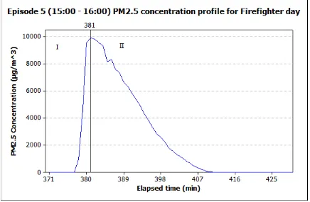
Figure 3-7: PM2.5 concentration profile during the last episode of the Firefighter day indicating regions of production and elimination: I-production, II-elimination ... 60
Figure 4-1: Indoor PM2.5 concentrations during the spring 2010 campaign ... 64
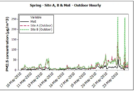
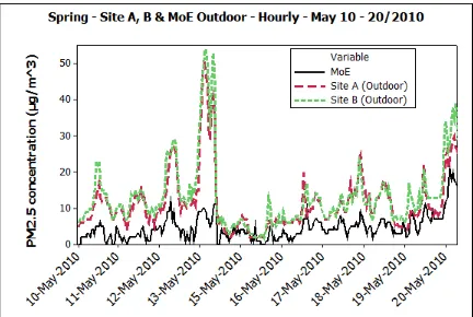
Figure 4-2: Spring - PM2.5 - Outdoor hourly concentrations ... 65
Figure 4-3: Spring - PM2.5 - Outdoor hourly concentrations, close-up... 66
Figure 4-4: Spring – Outdoor - Hourly PM2.5 correlation Site A and MoE ... 67
Figure 4-5: Spring – Outdoor – Hourly PM2.5 correlation Site B and MoE ... 68
Figure 4-6: Spring – Outdoor – Hourly PM2.5 correlation Site A and Site B ... 68
Figure 4-7: Spring - PM2.5 – Site A - Indoor and outdoor hourly concentrations ... 70
Figure 4-8: Spring - PM2.5 – Site A - Indoor and outdoor hourly correlation plot ... 71
Figure 4-9: Spring - PM2.5 – Site B - Indoor and outdoor hourly concentrations ... 73
Figure 4-10: Spring - PM2.5 – Site B - Indoor and outdoor hourly correlation plot ... 75
Figure 4-11: PM2.5 concentrations during the winter 2010 campaign, Site A & B – indoor ... 76
Figure 4-12: Winter campaign - PM2.5 concentrations between 5:30 am to 8:30 am on Monday mornings ... 86
Figure 4-13: Spring campaign - PM2.5 concentrations between 5:30 am to 8:30 am on Monday mornings ... 87
Figure 4-14: Winter campaign - PM2.5 - MoE hourly concentrations ... 90
Figure 4-15: Spring campaign - PM2.5- MoE hourly concentrations ... 91
Figure 4-16: Winter Campaign - Site A & B - NO2 average concentrations ... 92
Figure 4-17: Spring Campaign - Site A & B - NO2 average concentrations ... 93
Figure 4-18: Spring - CO2 concentrations vs. time ... 95
Figure 4-19: Friday May 21 - CO2 concentration ... 97
Figure 4-20: Monday May 24 - CO2 concentration ... 98
Figure 4-21: Tuesday May 18 to Wednesday May 19, CO2 concentrations ... 99
Figure 4-22: Site A indoor PM2.5 concentrations during Firefighter demonstration day – Feb/19/2011; Five different episodes are observed ... 100
Figure 4-23: Episode 2 of the Firefighter day PM2.5 concentration profile identifying the production and elimination areas. ... 102
Figure A-1: Schematic diagram of a single-channel PM2.5 FRM sampler (Source USEPA, 1997) ... 119
Figure C-1: Winter correction factor from inter-instrument variability test ... 124
Figure C-3: Spring PM2.5 pre inter-instrument comparison DT3 and DT4 ... 126
Figure C-4: Spring campaign, post study PM2.5 inter-instrument comparison ... 127
Figure C-5: Spring campaign, CO2 post study inter-instrument comparison, concentration vs. time ... 129
Figure F-4: Cumulative probability distribution plot and Anderson-Darling statisitic for Site A – indoor, Spring ... 134
Figure F-5: Cumulative probability distribution plot and Anderson-Darling statisitic for Site B – indoor, Spring... 136
Figure F-6: Cumulative probability distribution plot and Anderson-Darling statisitic for Site A – indoor, Winter ... 138
Figure F-7: Cumulative probability distribution plot and Anderson-Darling statistics for Site B – indoor, Winter ... 139
Figure G-1: Episode 2 PM2.5 concentration profile ... 140
Figure G-2: Episode 2 PM2.5 production profile ... 141
Figure G-3: Episode 2 PM2.5 elimination profile ... 141
Figure G-4: Episode 4 PM2.5 concentration profile ... 142
Figure G-5: Episode 4 PM2.5 production profile ... 142
Figure G-6: Episode 4 PM2.5 elimination profile ... 143
Figure G-7: Episode 5 PM2.5 concentration profile ... 143
Figure G-8: Episode 5 PM2.5 production profile ... 144
NOMENCLATURE
LIST OF ABBREVIATIONS
AADTC Annual Average Daily Traffic Count
AD Anderson Darling statistic
ASHRAE American Society of Heating, Refrigerating and Air-Conditioning Engineers
CO Carbon Monoxide
CO2 Carbon Dioxide
CWS Canada-Wide Standard
EC Elemental carbon
FEV Forced expectorant volume
GIS Geographical information system
GPS Global positioning system
HCHO Formaldehyde
HNO3 Nitric acid
HVAC Heating Ventilating and Air Conditioning LOD Limit of Detection
MDL Minimum detection limit
MoE Ministry of the Environment
NAAQS National Ambient Air Quality Standards
NH3 Ammonia
NH4NO3 Ammonium nitrate
NO2 Nitrogen Dioxide
OC Organic carbon
PEM Personal equipment monitor
PM Particulate Matter
PM2.5 Particulate matter with aerodynamic diameter equal or less than 2.5 microns
PM10 Particulate matter with aerodynamic diameter equal or less than 10 microns
ppm parts per million (concentration) PSCF potential source contribution function
SO2 Sulfur Dioxide
SVOC Semi Volatile Organic Compounds TEOM
TSP Total Suspended Particles
TVOC Total Volatile Organic Compounds
UFP Ultrafine particles
USEPA United States Environmental Protection Agency
CHAPTER 1 - INTRODUCTION
1.1. Background
Air pollution in Canada is a critical environmental and public health concern because of
the many health effects associated with our exposure to it. Past studies show correlations
between exposure to air pollution and premature mortality and morbidity (Horstman et
al., 1982; Linn et al., 1986; Lin et al., 2002; Pope et al., 2006; OMA, 2008). Not all age
groups react the same to air pollution exposure. Some age groups, in particular, infants,
children and the elderly are more susceptible. According to the American Academy of
Pediatrics (Kim, 2004), children are more susceptible to air pollution because of their
increased level of exposure, higher lung ventilation rates and higher levels of physical
activity. Children are also more vulnerable to the characteristics of local built
environments due to their mobility constraints and parental controls i.e., their inability to
control the time spent in a particular environment.
There is an ongoing need to study the levels of air pollution which are considered
dangerous to our health as recent reports have identified adverse health effects at levels
near or below the current standards for ozone, particulate matter and nitrogen dioxide
(Kim, 2004). Even though the Canadian Environmental Protection Act came into force
on March 31, 2000 (Environment Canada, 2011), the air in many parts of Canada is not
all considered clean. In Ontario, the air quality is better in some areas compared to others
(Environment Canada, 2004). The air quality in some micro-environments is different
concentrations compared to rooms where less ventilation is available. In order to better
predict the air pollution levels in different micro-environments more research is needed to
determine the concentration levels across multiple micro-environments or the exposure
levels at each of the micro-environments where the concentrations are already known.
Children spend much time in different micro environments each day, such as at home,
outdoor when walking to school, in classrooms, in a gymnasium, school surroundings,
inside a bus or private vehicles, shopping centers with parents, and others. It is
imperative that more information is gathered on the typical concentrations observed in
such environments so that norms and standards of acceptable levels can be established.
While many past studies focused on gathering air pollution exposure data in children’s
indoor environment, such as the school classroom (see Chapter 2 for in depth
description), only a handful of studies examined the relationship between indoor activity
in a school gym and particulate matter (PM) concentrations. In elementary schools,
physical education is a mandatory activity and it usually takes place inside the school
gym for most months of the school year. Very little data is available regarding the air
quality inside school gyms. Since indoor PM concentration is a function of ambient
concentration plus indoor concentration, and children spend time inside the gyms on a
daily basis, knowing the concentration inside the gyms is important in order to accurately
1.2. Objective
This thesis presents some of the results from a larger study entitled “Emerging
Methodologies for Examining “Environmental Influences on Children’s Exposure to Air
Pollution.” The study was conducted by a team of researchers from the University of
Western Ontario in collaboration with the University of Windsor. The short term goal of
the study was “to develop and test a new and improved methodology for measuring
children’s exposure to air pollutants in urban environments” (Gilliland et al., 2009). The
long-term, on-going goal of the project is “to better identify how characteristics of
physical environments impact children’s activities and exposure to air pollutants” so that
recommendations and interventions (behavioral or environmental) can be brought
forward in order to improve children’s health and quality of life. The study gathered air
pollution data using personal equipment monitors (PEM) mounted to participants, indoor
(inside the elementary school gymnasiums) and outdoor active PM2.5 monitors, passive
NO2 monitors surrounding the schools and areas where the majority of the school
attending children live and CO2 monitors inside the gyms. The study also gathered
comprehensive data on the participants by using daily activity questionnaires,
accelerometers mounted on each participant, global position system (GPS) instruments,
and before and after the study one-on-one interviews. Physical measurements and health
conditions were gathered for each participant prior to the start of the study.
This research presents the results of two, three-week sessions, of continuous monitoring
• To collect PM2.5, NO2 and CO2 data by installing active and passive monitoring
equipment in and around the elementary schools in question
• To determine if indoor PM2.5 concentrations in the gyms were higher than
outdoors
• To determine the effect of the following factors on PM2.5 in the gyms:
o Activity vs. no-activity
o Ventilation on/off
o Weekday/weekend
o Seasonal differences
o Location of gym inside the building
o Outdoor PM2.5 concentration
o Outdoor NO2 concentration
o Indoor CO2 concentration
• To determine which of the above mentioned factors has the largest influence on
CHAPTER 2 - LITERATURE REVIEW
2.1. Sources of Particulate Matter
2.1.1. General characteristics of Particulate Matter
Particulates, also referred to as particulate matter, are a small discrete mass of solid
and/or liquid matter that remain individually dispersed in gas or liquid emissions and are
suspended in the air (Jacobson, 1999). Aerosols and raindrops are all considered
particles. Airborne particles represent a complex mixture of organic and inorganic
substances. They directly and indirectly affect air quality, meteorology, climate and
human health.
The size of these particles tends to divide them into mainly two groups: coarse particles
and fine particles. Coarse particles are larger than 2.5 micro meters (µm) in aerodynamic
diameter while fine particles are smaller than 2.5 µm in aerodynamic diameter (PM2.5).
The aerodynamic diameter is referred to as the size of a unit density sphere with the same
aerodynamic characteristics. The particles are sampled and described on the basis of
their aerodynamic diameter which is simply called the particle size. Particles are
classified by their diameter because their size governs:
• The transport and removal of the particles from the air
• The deposition within the respiratory system
• The association with the chemical composition and sources
Figure 2-1 displays the diameter of multiple items in an effort to visually show the sizes
referred to based on its diameter as: inhalable, thoracic (≤PM10), and respirable (≤PM2.5)
(WHO, 2000).
Figure 2-1: Comparison of multiple objects of different size distributions (USEPA, 2011)
Figure 2-2 displays an idealized distribution of ambient particular matter (USEPA, 2004).
The size of suspended particles in the ambient air varies over 4 orders of magnitude, from
nanometers (nm) to micrometers (µm). The largest of particles are called the coarse
fractions and are produced by the mechanical break-up of larger solid particles. The
energy amount required to break up these particles into smaller sizes increases as the size
of the particle decreases, as a result, the lower limit of the production of the coarse
Figure 2-2: Size distribution of ambient particulate matter (USEPA, 2004)
There are two sources of coarse PM, natural and man-made. Natural sources of particles
include volcanic eruptions, fire, wind induced dust, ash and pollen. Man-made sources
consist of material handling (dust), smoke, fumes, dust from unpaved roads, power
plants, industrial and mining operations. Road dust is produced by traffic and air
turbulence can re-entrain it into the atmosphere. The evaporation of sea spray can
produce large particles along coast lines. Other coarse type particles include pollen
grains, mould spores, plant and insect parts (WHO, 2000). When measuring the chemical
composition or particles in the air, the particle mass can be classified according to various
2.1.2. Fine Particulate Matter
Particles smaller than or equal to 2.5 µm in aerodynamic diameter are considered fine
particulate matter. Within this category, particles smaller than 0.1 µm in aerodynamic
diameter are further classified as ultrafine particles (UFP), also referred to as the fine
fraction. They are formed by the condensation of low vapor-pressure substances, by high
temperature vaporization or by chemical reactions in the atmosphere (Jacobson, 1999).
These particles grow in size by a process called coagulation or by condensation. Because
coagulation is mostly efficient for large numbers of particles and condensation is mostly
efficient for large surface areas, the efficiency of these processes decreases as the size of
the particles increases. The upper limit to these processes is around 1 µm. Particles
between 0.1 µm and 1 µm tend to accumulate, thus this range is referred to as the
accumulation range (World Health Organization, 2000).
The smaller PM2.5 particles contain metal and recondensed organic vapors, combustion
particles and secondary reaction aerosols. Particles under 1 µm can be produced by the
condensation of metals or organic compounds which are vaporized from high
temperature combustion processes. They can also be produced by the condensation of
gases such as sulphur dioxide (SO2) in the atmosphere which oxidizes to form sulphuric
acid (H2SO4), or nitrogen dioxide (NO2) which oxides to nitric acid (HNO3). Nitric acid
reacts with ammonia (NH3) to form ammonium nitrate (NH4NO3). These particles,
which are produced by secondary reactions are called secondary reaction particles.
Secondary particles are the dominant component of fine particles. From the relationship
the total mass, however at the same time contributing over 90 percent of the total particle
number (Jacobson, 1999).
Trans-boundary air pollution of man-made pollutants and natural occurrences (such as
forest fires or volcanoes) caused by wind moving fine particles from the source location
can also be considered sources. Zhou et al. (1995) and Sapkota et al. (2005) describe
large trans-boundary pollution events that carried particles from the source more than a
few thousand kilometers to where they were being recorded.
2.2. Particulate Matter and human health
2.2.1. Health effects associated with exposure to PM2.5
To date, different effects of PM on health have been reviewed by many countries and
organizations (World Health Organization, 2000). This section provides a brief overview
of some of the research conducted regarding the association between air quality and
multiple health conditions. It is outside the scope of this research to provide a detailed
summary into any of the categories mentioned. Results from multiple studies suggest
that associations between PM10, total suspended particles (TSP) and mortalities observed
may very well be due to the effects of fine rather than coarse particles. Due to the focus
of this research on PM2.5, studies involving coarse particles (≥ PM2.5) and their effects on
health (e.g., Samet et al., 2000; Goldberg et al., 2001) have been omitted. Many studies
have shown that generally PM2.5 is a better predictor of health effects than PM10 (particles
Controlled studies
Data from controlled human exposure to PM is limited to sulfuric acid and acid sulfates
in normal and asthmatic subjects. In subjects exposed to PM for several hours, while
performing intermittent exercise, studies show a general agreement that inhalation of
sulfuric acid mists (1µm or less in diameter) in concentrations of up to 100 µg/m3 does
not cause any changes in lung function (Kerr et al., 1981; Horstman et al., 1982). Other
studies reported very little response to exposure of concentrations up to 1500 µg/m3 of
sulfuric acid mists of the specified size (Utell et al., 1984; Avol et al., 1988). Petrovich et
al. (2000) reported that exposure of young healthy volunteers to levels of concentrated
ambient PM2.5 in Toronto may not cause significant acute health effects. Their study
reported only a small mean decrease of 6.4% in thoracic gas volume after exposure to
high levels of PM2.5 concentrated from ambient air.
Asthmatics subjects have been reported to be more sensitive to exposure of sulfuric acid,
although the findings from different studies vary considerably. Some studies report no
changes of mean lung function after exposures to concentrations of up to 3000 µg/m3,
much like normal subjects (Linn et al., 1986; Aris et al., 1991). Other studies have
reported bronchoconstriction at concentrations below 1500 µg/m3 but above 380 µg/m3
(Utell et al., 1983; Avol et al., 1988). Out of these studies, forced expectorant volume
(FEV) in asthmatic subjects fell by 4.5% after exposure to 1000 µg/m3 of sulfuric acid
and there was a 20% reduction in specific airway conductance whereas the normal
studies due to different study designs and different modes of delivery and particle size of
the sulfuric acid used.
Epidemiological studies
Traditionally, epidemiological studies have played an important role in deriving guideline
values for acceptable levels of airborne PM. Concerns about the health effects of
airborne particles are based largely on the results of epidemiological studies suggesting
effects on mortality and morbidity at low levels of exposure. This section provides a
brief review of some epidemiological studies relating PM2.5 exposure to various health
endpoints.
One of the most recently published studies is the work of Pope and Dockery (2006).
They reviewed six substantial lines of research published until 1997 that have helped our
understanding of PM effects on health. The six lines were:
• Short-term exposure and mortality
• Long-term exposure and mortality
• Time scales of exposure
• Shape of concentration-response function
• Cardiovascular disease, and
• Biological plausibility
Based on a number of studies, the review concluded that the people who are most
asthma, especially the young and the elderly are most likely to be susceptible from
short-term exposures to moderately elevated PM concentrations. Different research teams,
using various analytical methods observed “consistent associations between
cardiopulmonary mortality and daily changes in PM.” Exposure to PM over long periods
of time has more persistent cumulative effects compared to short-term transient exposure.
Time-series studies
Time-series studies attempt to relate the development of air pollution with time to some
health variables such as daily mortality and hospital admissions for various symptoms.
They are largely snapshots that try to find a relationship between the air pollution at a
given time to various health endpoints. Data for these studies are routinely collected
through various programs and air pollution levels are used as exposure variables. The
sources for the health data vary, but are usually retrieved from hospital admissions and
routine statistical data among other more complex methods (WHO, 2000).
There are some methodological issues with the time-series analysis, such as the need to
adjust for weather and seasonal cycles. For example, winter months have higher
mortality rates much like heat waves do in summer months. Weather affects both air
pollution concentrations and health, making it difficult to adjust the associations of health
effects to either variable. The advantage of time-series studies is that they focus on
relatively short periods of days or weeks. Potential confounders such as age and smoking
habits do not change over the range of such studies thus they can be ignored. According
amount of time studied is often much greater than the variation in the long-term average
pollution concentration which forms the basis of long-term effects of air pollution health.
Hospital admissions
A study by Thurston et al. (1994) examined air pollution and daily hospital admissions
for respiratory causes in Toronto, ON. Ozone, PM2.5, PM10 and TSP data were obtained
for the months of July and August from 1986 to 1988. Daily counts of respiratory
admissions from 22 acute care hospitals during the same time period were also obtained.
The study found that associations decreased in strength from hydrogen ion to sulfates to
PM2.5 to PM10 to TSP, thus indicating that particle size and composition are important in
defining the adverse human health effects associated with PM. It was found that
summer-time haze was associated with roughly half of all respiratory admissions.
No studies have been able to make judgment on concentrations below which there are no
health effects. However, effects on mortality, respiratory and cardiovascular admissions
and other health end-points have been observed at levels well below 100 µg/m3.
Prevalence of bronchitis symptoms in children and reduced lung function in children and
adults have been observed at annual average concentration levels below 20 µg/m3 for
PM2.5 and were considered to be related to PM.
2.3. Particulate matter standards around the world
Canada-Wide Standard (CWS) for PM2.5 is 30 µg/m3. The standard is over a 24-hr
averaging time and it is based on the 98th percentile ambient measurement annually,
averaged over 3 consecutive years (Canadian Council of Ministers of the Environment,
2000). The U.S. has two different PM2.5 standards (USEPA). The annual (arithmetic
mean) based on the 3-year average of the weighted annual mean PM2.5 concentrations
from single or multiple-oriented monitors must not exceed 15 µg/m3. The 24-hr average
conditions are identical to those of the CWS except they must not exceed 35 µg/m3
(USEPA, 2004). Unlike Canada, the U.S. also has a PM10 24-hr standard of 150 µg/m3;
this is not to be exceeded more than once per year on average over 3 years. The
European Union (EU) shares the standards with the World Health Organization (WHO).
The EU PM2.5 limit has an averaging time of 1 year and it is based on a 3-year running
annual mean. The Australian limits are just guidelines for the time being. China has
three different 24-hr PM10 standards based on grades (CAI Factsheet No. 2, 2010).
Grades are essentially a different way to designate areas (i.e., Grade I is reserved for
natural conservation areas while Grade III is for special industrial areas). PM2.5 standards
do not exist at the moment in China, this is also the case with other Asian countries such
as Malaysia, Indonesia and the Republic of Korea. The allowable PM2.5 and PM10
Table 2-1: Particulate matter criteria from a few countries
Pollutant Canadaa United
Statesb EU
c
Australiad Chinae
PM2.5 30 15/35 25 25 -
PM10 - 150 40/50 50 50/150/250
a
Canadian Council of Ministers of the Environment
b15
µg/m3 annual, 35 µg/m3 over 24-hr
c40
µg/m3 annual, 50 µg/m3 over 24-hr
dNational Environment Protection (Ambient Air Quality) Measure – goal only
eChina Grade I, Grade II and Grade III, respectively
2.4. Methods of measuring particulate matter
There are multiple methods of measuring particulate matter of different size fractions.
This section explains the methodology behind two of the more recognized and commonly
used instruments along with one reference method. Most instruments either use
gravimetric analysis or light scattering as a means of obtaining PM concentrations.
Gravimetric analysis is a method commonly used to determine the mass of a solid. When
it comes to determining PM concentration, it essentially involves the weighing of a filter
before and after the filter is used. The difference in the weight of the filter is the total
accumulated PM. Using the total flow of the air over the collection media (filter) the
concentration can be calculated simply by dividing the weight by the volume of air
circulated. This method can be very accurate depending on the accuracy of the scale used
to weigh the collection media and depending on how well the quality control protocol
treated filter or devices such as a denuder. In order to obtain the composition of that
pollutant (e.g., % Pb, Elemental Carbon, Organic Carbon in PM2.5), the method has to be
paired with other more sophisticated chemical analyses (Parikh, 2000), such as X-ray
fluorescence.
2.4.1. Federal Reference Method
The Federal Reference Method (FRM) is the USEPA designated method for measuring
PM2.5 concentrations. It is defined in the Federal Register Appendix L – Part 50
(USEPA, 1997). The method states that only measurements made using USEPA
designated instruments and methods may be referred to and reported as PM2.5.
Measurements using other instruments and methods may not be accepted into the Federal
database as PM2.5. The method describes PM2.5 samplers and breaks them down into
reference samplers and three classes of equivalent sampling/measuring devices. The
main facets of the method are presented in Appendix A.
2.4.2. Tapered Element Oscillating Microbalance Procedure
The tapered element oscillating microbalance (TEOM) is an instrument that was
manufactured by Rupprecht and Patashnick (R&P) prior to it being acquired by the
Thermo Scientific group (Environmental Data Pages, 2011). The most popular model
used is the R&P 1400a TEOM. The instrument is still used to date by many U.S.
departments as well as different ministries of the Canadian government. The instrument
is cited with the FRM PM2.5 sampler (Parikh, 2000). This instrument is a “true”
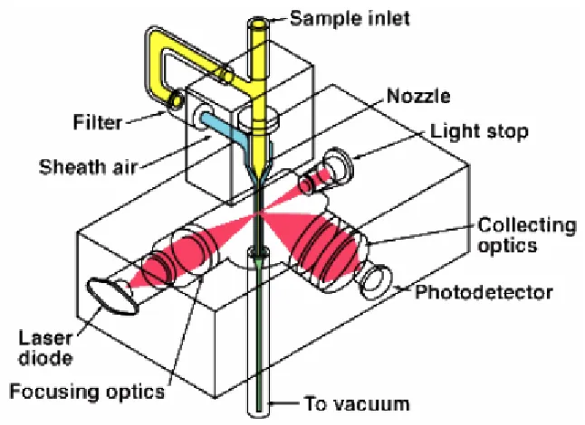
2.4.3. DustTrak 8520
The DustTrak, model 8520 is a PM measuring instrument manufactured by TSI
Incorporated (TSI, St. Paul, MN, USA). It uses a simpler physics principle in its design
compared to the TEOM and it is mostly used in the health and safety industry as well as
occasional research studies because it provides reliable concentrations with portability,
easy operation and maintenance.
Theory of operation
The DustTrak uses light scattering technology to determine mass concentration in
real-time. The aerosol sample is drawn into the sensing chamber in a continuous stream at 1.7
lpm. One section of the aerosol stream is illuminated by using a small beam of laser
light. The particles scatter light in all directions. A lens placed at 90° to the aerosol
stream and laser directs some of the scattered light and focuses it on the photodetector.
This light is in turn converted into a voltage. The voltage is proportional to the light
scattering which is in-turn proportional to the concentration of the aerosol sample. The
end voltage is multiplied by an internal calibration constant to yield mass concentration.
The internal calibration constant is determined from the ratio of the voltage response to
the known mass concentration of the test aerosol. The unit is calibrated against a
gravimetric reference using A1 test dust (ISO 12103-1, Arizona Test Dust). The laser
diode in this model has a wavelength of 780 nm which limits the smallest detectable
resolution equal to 0.001 mg/m3 (1 µg/m3). If the averaged concentrations are below, the
instrument will display a 0.000 mg/m3.
The instrument has been used in numerous studies around the world (Yanosky et al.,
2002; Evans et al., 2008; Diapouli et al., 2008; Wallace et al., 2010) some of which are
further discussed in this thesis. A study published by Wallace et al. (2010) found that the
limit of detection (LOD) derived using measured means and standard deviations (SD) for
the DustTrak is actually 5 µg/m3, unlike the manufacturer’s much lower claim.
According to the study, values lower than the minimum detection limit (MDL) are not
distinguishable from zero. The instrument is not approved under the FRM. Figure 2-3
displays the general schematics of the DustTrak 8520. Although this type instrument is
not as accurate as gravimetric monitors, it still provides useful information for risk
management and the effect of different micro-environments on personal exposure
Figure 2-3: Schematics of DustTrak 8520 (Courtesy of TSI Inc.)
2.5. Studies on the exposure to indoor air pollution
Building occupants today are exposed to chemical sources that are different from the
sources that occupants were exposed to 50 years ago. By knowing the differences
between these chemicals we can determine the effects that pollutants have on multiple
aspects of human health. A study by Weschler (2009) attempted to identify the changes
of these indoor chemicals since the 1950’s. The study concluded that over the last 50+
years, indoor exposure to known carcinogens (e.g., benzene, formaldehyde, asbestos,
environmental tobacco smoke and radon) and “reasonably anticipated” carcinogens
(chloroform, trichloroethylene, carbon tetrachloride and naphthalene) has decreased.
However, exposure to endocrine disruptors (e.g., certain phthalate ester plasticizers,
and mercury (Hg) have also declined. The study further concludes that there is very little
year to year data on the concentration of indoor air pollution particularly on semivolatile
organic compounds (SVOC) and their effect on human health. The author suggests the
establishment of monitoring networks that provide information about the state of
pollutants in representative buildings working in conjunction with outdoor pollutant
monitors and body fluid monitors. This would “enhance our knowledge of the chemicals
that we inhale, ingest and absorb on a daily basis.”
Lin et al. (2007) presented the emissions of 2,2,4-trimethyl-1,3-pentanediol
monoisobutyrate (TMPD-MIB) from two types of latex paints (regular and glossy
finishes) applied to aluminum, gypsum board and concrete. TMPD-MIB, also referred to
as Texanol® ester alcohol, is a type of VOC. The study concluded that air emissions that
were released the longest time were from gypsum board, with concrete and aluminum
emitting less in that order.
2.6. PM2.5 in elementary schools
2.6.1. Studies of PM2.5 in elementary school classrooms
There have been many studies whose goals have been the reporting of indoor PM
concentrations in elementary school classrooms. Attributable to the focus of the research,
this section describes some of the results from PM2.5 only studies, and excludes results
from other PM studies. Some studies measured both PM2.5 and PM10 concentrations.
Scheff et al. (2000) measured and evaluated the indoor air quality at a middle school in
Springfield, Illinois. Integrated samples with an eight hour sampling time for respirable
(PM2.5) and total particulate matter, short-term measurements for bioaerosols and
continuous CO2 logging were collected on three consecutive days during one week in
February of 1997. Four indoor locations: the cafeteria, a science classroom, an art
classroom and the lobby outside of the main office, were sampled. The school was
located in an area with no known air quality problems. The science room showed the
highest average PM2.5 concentration of 30 µg/m3 over the three days while the art
classroom showed the lowest concentration of 14 µg/m3. The study concluded that there
was a linear relationship between occupancy and corresponding CO2 and particulate
concentrations and those concentrations are influenced by the indoor spaces in which
they are measured.
Three elementary schools around Columbus, Ohio (one rural, one suburban and one
urban site) were monitored for indoor and outdoor PM2.5 air quality from February 1,
1999 through August 31, 2000 (Kuruvilla et al., 2007). Indoor PM2.5 monitors were set
to run from 8:00 am – 3:00 pm Monday-Friday for the entire school year while the
outdoor measurements used the TEOM instrument described earlier. The mean indoor
PM2.5 concentrations at the suburban and rural sites were higher than those observed
outdoors at these sites, while the outdoor concentration was higher than the indoor PM2.5
level at the urban location. However, this pattern was not consistent during the entire
and on potential source contribution function (PSCF) analysis. It was concluded that
PM2.5 levels did not exceed the National Ambient Air Quality Standards (NAAQS)
during the entire study and the PSCF analysis provided a reasonable estimate of the
influence of upwind regions on PM2.5 contribution. Although the study did identify SO4
2-as the single largest component of PM2.5 mass contributed, it did not explain the potential
health implications on children of all the pollutants measured.
In an air quality study aimed at assessing base-line concentrations of indoor air quality in
Antwerp, Belgium, 18 residences and 27 primary schools were evaluated for different air
pollutants including PM2.5 and PM10 (Stranger et al., 2007). The 27 schools were
composed of 15 inter-city schools and 12 schools from surrounding suburban areas 20
km south of Antwerp. Particulate matter was collected during two sampling campaigns
(autumn-winter and spring-summer) from December 2002 to June 2003. A gravimetric
method was used for a 12-hr period from Monday to Friday only. The average 12-hr
indoor PM2.5 concentration for the 27 schools was 61 µg/m3, with a range of 11-166
µg/m3. This concentration exceeded observations from other studies and is twice that of
the CWS. However, it should be noted that they were only 12-hr measurements and thus
cannot be directly compared to some standards.
PM10 and PM2.5 size fractions were measured gravimetrically inside two classrooms as
well as outdoors at one primary school in northern Munich, Germany for 6 weeks during
the months of October and November of 2006 (Fromme et al., 2008) for 5 hours a day.
was estimated that 43% of PM2.5 was of ambient origin. The study concluded that PM
measured in classrooms has major sources other than outdoor particles and that PM
generated indoors may be less toxic compared to PM in ambient air.
2.6.2. Studies of PM2.5 in school gymnasiums
Research of indoor PM2.5 air quality in school gymnasiums has been minimal. Past
studies dealing with air quality in schools are almost entirely concerned with classrooms
as already mentioned. Search results do not reveal a lot of studies aimed at directly
evaluating the air quality in the gyms but rather at evaluating the air quality within the
schools and surrounding areas. As a result, most studies report the PM2.5 concentration in
the classrooms. However, a few limited studies did focus on the “exposure of children to
airborne particulate matter of different size fractions during indoor physical education at
school.” A detailed summary of studies that report PM2.5 monitoring in school gyms is
presented in this section because of their relevance to the current study.
The Prague, Czech Republic School Study
The study of Branis et al. (2009) was designed to document the exposure of children
between the ages of 11-15 years to PM2.5 during scheduled indoor physical exercise. The
gym was in a naturally ventilated school with an “expected high infiltration” rate of
outdoor air. The school was situated in the city centre of Prague, Czech Republic. The
location was chosen because of its high traffic congestion frequency. The main source of
of indoor-outdoor relationships, possible indoor PM2.5 sources and potential health effects
associated with the recorded levels of aerosol in the indoor environment.
The city of Prague is the capital of the Czech Republic. It has a population of 1,250,000
and it lies at an altitude between 200 and 350 m above sea level which is comparable to
the city of London, ON. The school was in a central location, with an approximate
distance of 100 m to the nearest main road. According to 2006 statistics, the traffic
density on this road was about 13,200 cars between 6 am and 10 pm on a working day.
The gymnasium dimensions are 16.6 m x 7.2 m x 4.9 m. It is a naturally ventilated space
with six large double-glazed windows. Gymnasium activity starts around 8 am. The
school and its surrounding area are strictly non-smoking. Particulate matter
concentrations were measured by a cascade impactor with 5 stages A to F (A: 2.5-10 µm;
B: 1.0-2.5 µm; C: 0.5-1.0 µm; D: 0.25-0.5 µm; and a final stage F: <0.25 µm). One 25
mm PTFE filter was used for stages A-D and a 37 mm PTFE filter was used for the final
stage. The inlet of the impactor was placed at a height of 2 m above the gym floor.
Filters were changed daily before the beginning of activities. The air flow of the
impactor pump was checked before and after each campaign.
Monitoring took place between November 2005 and August 2006 and it was divided into
8 campaigns, each between 7-10 days. PM2.5 ambient concentrations were obtained from
a fixed site monitor of the national air quality monitoring system located about 3.3 km
Activity in the gym was recorded along with the number of persons present and the
duration of the activity, using a written form attached to the front of the gym door. The
total PM2.5 concentration was determined by summing stages B – F, excluding stage A
which measured only the coarse fraction. Indoor and outdoor concentrations were paired
and compared using the Mann-Whitney U test.
The average and median indoor PM2.5 concentrations for all 8 campaigns were 24 and 25
µg/m3 respectively. These were similar to the outdoor monitor, which recorded 25.5 and
23.75 µg/m3, respectively. The difference between the two data sets was not significant
(p=0.81). Even though the fixed site monitor was located 3.3 km from the school, the
correlation coefficient between the two data sets was 0.88, suggesting a homogeneous
dispersion of pollutants within the city as well as a high infiltration rate indoors. The
correlation coefficient of the smaller PM2.5 size fractions with the fixed site monitor was
greater than the coarse aerosol correlation (0.88 vs. 0.46). This indicated that a
signification portion of the indoor PM2.5 aerosol had its origin outdoors.
The regression equation between the two variables (indoor vs. outdoor) showed that more
than 60% of the indoor PM2.5 can be explained by the fixed site monitor (Indoor =
0.63*Outdoor + 8.08; R2=0.83). The study could not conclude which concentrations
were more accurate due to the different measuring techniques of the instruments used and
the location and distance between the instruments. The real concentration was
provided support for the significant influence of ambient particles on the indoor
microenvironment.
The Athens Elementary School Study
Diapouli et al. (2008) characterized the PM10, PM2.5 and UFP concentration levels at
elementary schools across Athens to examine the relationship between the indoor and
outdoor concentrations. Seven primary schools were chosen. The schools were
distributed through the surrounding areas of the city. The indoor air intake samples were
taken at table height. Three of the seven schools were monitored in multiple locations
such as: a computer lab in the library, a teacher’s office and the gymnasium. The outdoor
measurements were carried out in the yard of the schools, in an area not accessible by the
children for the security of the instrument. Each school was studied for 2-5 consecutive
weekdays during school hours, 8:00 am – 4:00 pm. PM10 and PM2.5 indoor and outdoor
concentrations were measured using Harvard personal equipment monitors (PEM) at a
flow rate of 4 lpm. Some schools used the DustTrak model 8520 to monitor PM10 and
PM2.5. UFP concentrations were measured using a TSI CPC3007 (Shoreview, MN,
USA). The TSI instruments were programmed to record the concentration every 1 min.
The indoor to outdoor ratio (I/O) for the site where the pollutants were measured inside
the school gym was 1.8 with indoor PM2.5 concentrations reaching as high as 80 µg/m3.
Libby Montana School Study
Ward et al. (2007) present the results of an indoor size fractionated PM school sampling
the only places in the western United States that exceeds the annual PM2.5 NAAQS. Two
schools, approximately 2.4 km apart were sampled during the months of January through
March of 2005 for indoor PM2.5 concentration. The sampling events (lasting 24 hr) were
simultaneously collected once per week for a total of 9 sessions. Only one of the schools
sampled was an elementary school. This school had the sampling instrument installed in
the gymnasium while the other school (a middle school) had the sampling instrument
inside a faculty supply room because the gymnasium was detached from the main
building. A Sioutas impactor PM sampler with Leland Legacy (SKC, Inc., Eighty Four,
PA) pump was fitted with Teflon filters to measure the gravimetric mass of five size
fractions (>2.5, 1.0-2.5, 0.5-1.0, 0.25-0.5, and <0.25 µm) of the indoor PM. Ambient
PM10 concentrations were measured simultaneously. The location of the outdoor
instruments was approximately 1.6 km from the elementary school.
The average indoor PM2.5 mass concentration at the elementary school was 41 µg/m3 over
the monitoring campaigns. This is approximately four times greater than the level
reported at the middle school. The authors attribute the difference in concentrations to
the age of the buildings (the elementary school was built in 1953 while the middle school
was built in 1970), and the difference in the sample locations (gymnasium vs. faculty
staff room) within the schools. Ambient PM10 concentration was not strongly correlated
with the elementary school or with the middle school (correlation coefficient [P-value] =
0.17 [0.69] and 0.10 [0.82], respectively), which can be explained by the fact that they
2.6.3. Study on the effects of building age on indoor PM concentration
In a study from South Korea (Yang et al., 2009), the concentrations of different indoor air
pollutants within 55 public schools were characterized to compare their indoor levels
with each other and to the number of years the school had been constructed. The study
was conducted in order to suggest ways of reducing the exposure of school children to
undesirable air pollutants. Indoor and outdoor air samples were obtained from three
different locations within the schools, a classroom, a laboratory and a computer lab. The
schools were selected based on the age of the building including 1, 3, 5 and 10 years old.
The data was gathered for 1 day at each location during summer, autumn and winter from
July to December 2004. The study measured concentrations for the following: CO, CO2,
PM10, TVOC’s and Formaldehyde (HCHO). The mean and standard deviation of PM10
for the entire study period were 77.87 and 68.90 µg/m3, respectively. The PM10
indoor/outdoor (I/O) ratio for the study period was 1.43, suggesting the major PM10
contributor was indoor. The study concluded that for PM10, building age did not show a
difference in mean concentrations. The mean concentrations were between 83.39 and
84.63 µg/m3 for the 4 building age groups. The limitations of the study included the lack
of direct PM2.5 measurements, a short monitoring period per school and no consequent
day to day measuring for each location. It was also limited to buildings not being older
than 10 years.
2.7. Summary
This chapter described some of the health effects associated with air pollution, general
research that already exists, it is apparent that increased levels of PM2.5 concentrations
can contribute to increased health problems in the adult population with severe
consequences towards children and the elderly. The next sections of this thesis present
the results related to the objectives outlined in Chapter 1. The school gym
micro-environments are just as important as shopping centres or daily walks to school since an
average child spends just as much time in them on a daily basis as they do in other more
CHAPTER 3 - MATERIALS AND METHODS
3.1. Study design
3.1.1. Site selection
General description
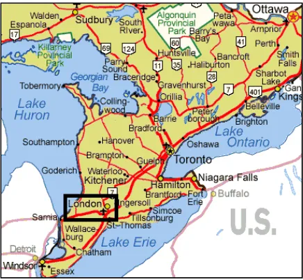
The study presented in this research took place in London, ON. The city is located in
South-Western Ontario. It has a metropolitan area population of approximately 492,000
making it the eleventh most populated city in Canada (Statistics Canada, 2007). It is
situated among the forks of the Thames River halfway between Windsor and Toronto at
an elevation of 270 m above sea level (Ministry of the Environment, 2011). Figure 3-1
displays the location of the city within the south-west part of the province of ON.
Figure 3-1: Position of London within South-Western Ontario (BEC Canada)
In order to identify and map potential “hot-zones” for ambient air pollution, land use
regression modeling techniques within a Geographic Information System (GIS) were
used (Luginaah et al., 2008). Two (2) elementary schools of varying outdoor
neighbourhoods were monitored to assess exposure to pollutants at two different time
periods (February/March and May 2010) to explore the impact of seasonality on potential
levels of exposure among students. The names of these elementary schools cannot be
disclosed and thus they are referred to as Sites A and B, hereafter shown in Fig. 3-2. Site
A was located in a sub-urban environment to the south of the city, approximately 1.6 km
north of Highway 401. Site B was located in an urban location close to city centre and
surrounded by some of London’s busiest roads.
The city of London’s monitoring site is located to the east of Site B. Outdoor ambient
concentrations, including PM2.5 and NO2 are continuously monitored by the MoE
(Ministry of the Environment, 2007). Figure 3-2 displays the location of both sites along
Figure 3-2: Sites A, B and MoE within the city of London
Gymnasium Characteristics
The oversized elementary school gym at Site A was built in 1972 with heavy renovations
to the entire school in 1995 along with the addition of another building. The gym is
placed in the center of the school with no direct contact to the outdoor environment with
the exception of the ceiling/roof. It is of rectangular shape with a total surface area of
423 m2. There are four different access doors to the gym. However, they all connect the
Site B’s gymnasium is attached to an elementary school built in 1949. There have been
no major renovations recorded in the school’s history. The gym is located to the south
west of the school’s geographical location and three of its walls are surrounded by the
outdoor environment. It is of a smaller size compared to Site A, and has a total surface
area of 278 m2 with two doors leading outdoors and one double size door leading to the
interior of the school. The main features of the schools and gyms are presented in Table
3-1.
Table 3-1: School and gym characteristics
School Area Ventilation # Doors/Entrances Area
(m2)
Building Age Site A Suburban, light traffic street nearby Mechanical
Four, all leading to the interior of the school 423 Built in 1972, renovated in 1995 Site B Urban, heavy traffic street in front Mechanical Two leading outdoors and one large leading inside the school
278 Built in 1949
Annual Average Daily Traffic Volume
The City of London traffic volume data (City of London, 2011) provided the Annual
Average Daily Traffic Count (AADTC) for the entire city including both sites. The
arterial street directly behind Site A, which runs parallel to Site A’s school yard has an
AADTC of 15,500 vehicles. Data for the street directly in front of Site A’s entrance was
3.1.2. Campaign schedule
The PM2.5 monitoring campaign took place during two different seasons, winter and
spring of 2010 for a total of approximately six weeks. The winter campaign started on
February 17th and ended on March 8th. The spring campaign continued from May 5th to
the 24th. Each season was monitored for approximately three weeks.
During the winter campaign, only indoor PM2.5 concentrations and ambient NO2
concentrations were measured. The first week of the spring campaign used the same
number of measuring equipment stations at approximately the same locations as the
winter. At the beginning of the second week of the spring campaign, two extra PM2.5
measuring instruments and three CO2 instruments were added. Thus, during the last two
weeks of the spring campaign both indoor and ambient PM2.5 concentrations were
recorded along with CO2 indoor and outdoor. Table 3-2 shows the monitoring schedule
for both winter and spring campaigns.
Table 3-2: Pollutant monitoring schedule; “I” and “O” represent indoor and outdoor monitoring, respectively
Week # Date (in 2010) PM2.5
NO2
(outdoor)
CO2
(indoor)
1 Feb. 17 - 22
(I)2 Feb. 22 - Mar. 01
(I)3 Mar. 01 - 08
(I)4 May 05 – 10
(I)5 May 10 – 17
(I & O) (I & O)Since the instruments were not started simultaneously at both locations due to the
logistics of the operation, the first and last days of the monitored weeks’ PM2.5 data were
eliminated from the analysis of both sites. The data eliminated did not capture a full
day’s worth of school activities and it consisted mainly of afterschool measurements.
3.2. Pollutant measurement
3.2.1. PM2.5 methodology
Measuring Method
PM2.5 concentrations were measured and recorded using the DustTrak Aerosol Monitor
model 8520. The instrument uses light photometry to detect particles. This procedure
was explained in greater detail in Chapter 2 of this thesis. Concentrations were averaged
over 1-min intervals and data was stored internally for up to two weeks at a time at which
point all data was downloaded into the field laptop. One unit was placed at each site in
the gymnasium during the winter campaign. In the spring campaign additional units were
set up to measure the outdoor concentrations during the last two weeks of the spring
monitoring campaign (Table 3-2).
Location of instrument within the gyms
The location of each instrument within the gyms was different relative to each gym’s
physical characteristics. Each unit was placed in a small, sealable bin with a short
Tygon® tube sticking out. The lengths of the tubes were similar and were shorter than
ensure optimal measuring accuracy. The bin was covered to protect the instruments from
various forms of daily activities.
Site A had the DustTrak placed in the middle of the gym, between the removable
dividing doors, on top of exercise mats. The height of the intake tube was approximately
1.8 m above floor level. Figure 3-3 displays the bin with the intake tube. For the spring
campaign, the height of the intake was lowered to about 1.2 m to be similar with Site B’s
set up and because the students started using the exercise mats.
Figure 3-3: Site A winter DustTrak set up
Site B’s DustTrak was placed in a small room adjacent to the gymnasium. The room
serves as a mini-cafeteria for various school activities and when not in use, it is mainly
used as a storage media for various goods. The room has a large sealable opening into
the gym. The intake tube was drawn into the gym and taped to the side of the wall. The