ABSTRACT
KACAR, NECIP BARIS. Developing and Fitting a Clearing Function: An
Experimental Comparison of A Clearing Function Model and Iterative Simulation-Optimization Algorithm for Production Planning of a Semiconductor Fab. (Under the direction of Professor Reha Uzsoy).
We address the fundamental problem of workload – dependent lead times in
production planning, known as planning circularity. We focus on a clearing function
model and iterative algorithm that addresses planning circularity. We develop a
clearing function form that expresses output as a function of the sum of the work
released within a period plus any work available at the start of the period. We develop
a new clearing function form which is different from the clearing functions based on
expected WIP over the period that have been previously studied. We implement our
clearing function form in the Allocated Clearing Function (ACF) model of (J. M.
Asmundsson, Rardin, R. L., Uzsoy, R., 2002) and compare its performance to that of
the Hung and Leachman (HL) procedure which is an iterative algorithm that combines
simulation and fixed lead time LP models. In our experimental comparison, we use a
simulation model of a re-entrant bottleneck system built with attributes of a real-world
semiconductor fabrication environment. We vary the bottleneck utilization, demand
patterns, the mean time to failure (MTTF) and mean time to repair (MTTR). Results
indicate that the ACF model using our clearing function form performs better than HL
procedure, giving less variable production plans and lower discrepancies between the
Developing and Fitting a Clearing Function Form: An Experimental Comparison of A Clearing Function Model and Iterative Simulation-Optimization Algorithm for
Production Planning of a Semiconductor Fab
by
Necip Baris Kacar
A thesis submitted to the Graduate Faculty of North Carolina State University
in partial fulfillment of the requirements for the degree of
Master of Science
Industrial Engineering
Raleigh, North Carolina March 2009
APPROVED BY:
______________________________ ______________________________
Dr. Yahya Fathi Dr. Brian Denton
________________________________ Dr. Reha Uzsoy
DEDICATION
To my family
who always supported and encouraged me
BIOGRAPHY
Necip Baris Kacar, was born in 1983 in Istanbul, Turkey. He graduated high
school from American Robert High School in 1999. He received his Bachelor of
Science degree in Mechanical Engineering from Bogazici University in 2003. Upon
graduation, He attended North Carolina State University for his Master of Science
degree in Industrial Engineering with minor in Operation Research. He is also working
as a Research Assistant for his professor Dr. Reha Uzsoy. He was elected to the Honor
Society of Phi Kappa Phi. He was the treasurer of Industrial and Systems Engineering
Graduate Student Association. His research interests include simulation based
optimization algorithms for production planning, capacity planning with
ACKNOWLEDGEMENTS
Most importantly, I would like to especially offer my gratitude to my advisor
Dr. Reha Uzsoy and appreciate his great support and excellent guidance in my
research. I truly thank you for giving the opportunity working with you and sharing
your vast knowledge with me.
I also would like to thank my other committee members Dr. Yahya Fathi and
Dr. Brian Denton for serving in my committee and their valuable comments regarding
my thesis.
I would like to recognize and thank to the entire faculty of Department of
Industrial Engineering in North Carolina State University who contributed to my
education. I also would like to recognize Hakan Sungur and Burak Eryigit, who work
in Department of Industrial Engineering, for their help and support in everything that I
need and offering their friendship to me. Thanks to all my friends in the department
and particularly to Nils Buch and Kuang-Hao Yeh (Claire) for being nice and good
TABLE OF CONTENTS
LIST OF TABLES ... vii
LIST OF FIGURES ... viii
CHAPTER 1. INTRODUCTION ... 1
CHAPTER 2. LITERATURE REVIEW ... 4
CHAPTER 3. ALGORITHMS COMPARED ... 8
3.1. Hung and Leachman (HL) Iterative Algorithm ... 8
3.1.1. LP Formulation ... 9
3.1.2. Steps of HL Iterative Algorithm: ... 13
3.2. Allocated Clearing Function (ACF) Model ... 14
3.2.1. LP Formulation ... 15
CHAPTER 4. EXPERIMENTAL DESIGN ... 19
4.1. Simulation Model ... 19
4.1.1. Simulation Parameters ... 21
4.1.1.1. Simulation Processing Times ... 21
4.1.1.2. Failure Distribution Parameters ... 22
4.1.2. Simulation Details ... 23
4.2. LP Models ... 23
4.2.1. Hung and Leachman Iterative Algorithm ... 24
4.2.2. Allocated Clearing Function (ACF) Model ... 26
4.3. Conversion of LP Releases to Simulation Input ... 27
4.4. Fitting Clearing Function ... 29
4.4.1. Data Collection for Fitting ... 29
4.4.1.1. Outline for Data Collection... 30
4.4.1.2. Plots of Empirical Data for Selected Machines ... 31
4.4.2. Fitting Clearing Function to Data ... 34
4.4.3. Does the Clearing Function depend on other schedules? ... 39
4.5. Experimental Factors ... 43
4.5.1. Bottleneck Utilization with Different Demand Patterns... 43
4.5.1.1. Constant Demand Pattern ... 44
4.5.1.2. Varying Demand Patterns ... 46
4.5.2. Length of MTTF and MTTR ... 47
4.5.2.1. Short Failure Case ... 48
4.5.2.2. Long Failure Case ... 48
CHAPTER 5. EXPERIMENTAL RESULTS ... 56
5.1. Performance Criteria ... 57
5.2. Short Failure Case ... 58
5.2.1. 90% Utilization Case ... 59
5.2.1.2. Constant Demand Case... 64
5.2.2. 70% Utilization Case ... 68
5.2.2.1. Varying Demand Case ... 68
5.2.2.2. Constant Demand Case... 72
5.3. Long Failure Case ... 75
5.3.1. 90% Utilization Case ... 76
5.3.1.1. Varying Demand Case ... 76
5.3.1.2. Constant Demand Case... 81
5.3.2. 70% Utilization Case ... 84
5.3.2.1. Varying Demand Case ... 85
5.3.2.2. Constant Demand Case... 88
5.4. Summary of Results ... 92
CHAPTER 6. CONCLUSION ... 94
6.1. Summary ... 94
6.2. Future Research Directions ... 96
LIST OF TABLES
Table 4.1: Simulation Processing Times and Batch Sizes... 21
Table 4.2: Failure Distribution Parameters ... 22
Table 4.3: Cost and Revenue Values... 26
Table 4.4: Cost Values of ACF Model ... 26
Table 4.5: Statistics of Fitted Linear Regression Lines... 38
Table 4.6: Failure Distribution Parameters for Long Failure ... 49
Table 4.7: Statistics of Fitted Linear Regression Lines for Long Failure ... 54
Table 5.1: ACF and HL Statistics LP Side for Short Failure 90% Varying Demand Case ... 62
Table 5.2: ACF and HL Statistics Simulation Side for Short Failure 90% Varying Demand Case ... 63
Table 5.3: ACF and HL Statistics LP Side for Short Failure 90% Constant Demand Case ... 67
Table 5.4: ACF and HL Statistics Simulation Side for Short Failure 90% Constant Demand Case ... 67
Table 5.5: ACF and HL Statistics LP Side for Short Failure 70% Varying Demand Case ... 71
Table 5.6: ACF and HL Statistics Simulation Side for Short Failure 70% Varying Demand Case ... 71
Table 5.7: ACF and HL Statistics LP Side for Short Failure 70% Constant Demand Case ... 74
Table 5.8: ACF and HL Statistics Simulation Side for Short Failure 70% Constant Demand Case ... 75
Table 5.9: ACF and HL Statistics LP Side for Long Failure 90% Varying Demand Case ... 80
Table 5.10: ACF and HL Statistics Simulation Side for Long Failure 90% Varying Demand Case ... 80
Table 5.11: ACF and HL Statistics LP Side for Long Failure 90% Constant Demand Case ... 83
Table 5.12: ACF and HL Statistics Simulation Side for Long Failure 90% Constant Demand Case ... 84
Table 5.13: ACF and HL Statistics LP Side for Long Failure 70% Varying Demand Case ... 87
Table 5.14: ACF and HL Statistics Simulation Side for Long Failure 70% Varying Demand Case ... 88
Table 5.15 ACF and HL Statistics LP Side for Long Failure 70% Constant Demand Case ... 91
LIST OF FIGURES
Figure 2.1: Examples of Clearing Functions (Karmarkar, 1989) ... 6
Figure 3.1: Flow chart of Iterative Algorithm of HL Procedure... 14
Figure 4.1: Re-entrant Bottleneck Model Process Chart for Products ... 20
Figure 4.2: Machine 1 Output vs. Resource Load ... 32
Figure 4.3: Machine 3 Output vs. Resource Load ... 32
Figure 4.4: Machine 7 Output vs. Resource Load ... 33
Figure 4.5: Machine 4 Output vs. Resource Load ... 33
Figure 4.6 : Machine 1 Linear Regression Fit ... 36
Figure 4.7: Machine 3 Linear Regression Fit ... 36
Figure 4.8: Machine 7 Linear Regression Fit ... 37
Figure 4.9: Machine 4 Linear Regression Fit ... 37
Figure 4.10: Intercept Comparison of Segment 1 ... 41
Figure 4.11: Slope Comparison of Segment 1 ... 41
Figure 4.12: Intercept Comparison of Segment 2 ... 42
Figure 4.13: Slope Comparison of Segment 2 ... 42
Figure 4.14: Constant Demand Pattern corresponding 90% Utilization ... 45
Figure 4.15 Constant Demand Pattern corresponding 70% Utilization ... 45
Figure 4.16: Varying Demand Pattern corresponding 90% Utilization ... 46
Figure 4.17: Varying Demand Pattern corresponding 70% Utilization ... 47
Figure 4.18: Machine 1 Output vs. Resource Load for Long Failure ... 49
Figure 4.19: Machine 3 Output vs. Resource Load for Long Failure ... 50
Figure 4.20: Machine 7 Output vs. Resource Load for Long Failure ... 50
Figure 4.21: Machine 4 Output vs. Resource Load for Long Failure ... 51
Figure 4.22: Machine 1 Linear Regression Fit for Long Failure ... 52
Figure 4.23: Machine 3 Linear Regression Fit for Long Failure ... 53
Figure 4.24: Machine 7 Linear Regression Fit for Long Failure ... 53
Figure 4.25: Machine 4 Linear Regression Fit for Long Failure ... 54
Figure 5.1: Schema of Experimental Factors... 56
Figure 5.2: ACF 90% varying demand short failure case product 1 LP and simulation outputs ... 59
Figure 5.3: ACF 90% varying demand short failure case product 2 LP and simulation outputs ... 60
Figure 5.4: ACF 90% varying demand short failure case product 3 LP and simulation outputs ... 60
Figure 5.5: HL 90% varying demand short failure case product 1 LP and simulation outputs ... 61
CHAPTER 1. INTRODUCTION
The goal of production planning is to match the output of manufacturing
facilities to customer demand in a way that optimizes the performance metrics of the
company. Manufacturing firms wish to control the timing of releases so that the
outputs are available when the customers need them. This requires knowledge of the
cycle time of the products, the time between the release of products into the plant and
their emergence as finished goods. However, an inherent problem in estimating the
cycle time is that it depends on the level of resource utilization in the system, which is
determined by the allocation of products to resources made by the production planning
procedure. This problem of workload – dependent lead times in production planning is
known as the planning circularity (J. M. Asmundsson, Rardin, Turkseven, & Uzsoy,
forthcoming), and has been studied by many authors (Pahl, Voss, & Woodruff, 2005).
In order address to this circularity problem, several production planning
models have been proposed. These models can be grouped under two main headings.
The first class of models considers lead time estimates as exogenous parameters
independent of resource utilization. The second class of models uses either detailed
scheduling algorithms or a simulation model to confirm that the release schedule
approach can capture the nonlinear relationship between the lead times and resource
utilization, but applying this approach to large scale problems may not be feasible.
One approach that uses a simulation model is to combine linear programming
(LP) and simulation in an iterative manner. Variations of iterative algorithms have
been proposed by several authors, including (Kim & Kim, 2001), (Byrne & Bakir,
1999), (Byrne & Hossain, 2005) and (Hung & Leachman, 1996). However, the
convergence behavior of these models is unclear and their computation time
requirements may be excessive due to the high computational burden of the detailed
simulation models.
In traditional capacity planning models, the nonlinear relationship between
work-in-process and output is not well captured. Thus, the effect of capacity loading
on flow times is not incorporated into the models. Given these shortcomings of
previous approaches, the idea of clearing functions which represent the expected
output of a resource over a period as a function of the expected work-in-progress
(WIP) has been proposed to capture the effects of load dependent lead times. These
models have been studied by a number of authors ((Graves, 1986), (Karmarkar, 1989),
(J. M. Asmundsson, Rardin, R. L., Uzsoy, R., 2002)) and have been shown to give
promising results in several studies. However, there is currently no broad agreement
on a systematic way to estimate the clearing functions for a given production system.
planning models based on clearing functions to those from iterative methods
combining LP and simulation models.
In this thesis, we focus on the problem of fitting clearing functions for a
specific set of production resources based on the resource load at the beginning of a
planning period, instead of the expected WIP level that has been used in previous
research. We examine the clearing function estimation in a different way, as a function
of the releases and WIP level at the beginning of a period. This approach is different
from using time average WIP to estimate the clearing function. By collecting data of
range of releases within a period and initial WIP levels and keeping the number of
outputs, we can estimate our clearing function by stating output as a function of
releases within a period plus initial WIP levels. In this thesis we investigate the
estimation of this type of clearing functions. After we estimate our clearing functions
in this manner, we incorporate these clearing functions in a production planning
model, and compare the performance of the clearing function models to those of
iterative models combining simulation and fixed lead time LP models.
In the next chapter, we provide a review of numerous previous related work in
production planning. In Chapter 3 we give a detailed description of the LP model of
Hung and Leachman procedure and partitioned clearing function model by (J. M.
Asmundsson, Rardin, R. L., Uzsoy, R., 2002). These are the two models that we
simulation model and steps of fitting clearing function. We also talk about our
performance criteria. Finally we present our experimental results and draw
conclusions based on our results. We finish our thesis with further research directions.
CHAPTER 2.
LITERATURE
REVIEW
There are numerous works in the literature presenting mathematical
programming models for production planning by allocating capacity to multiple
products over time while satisfying demand and optimizing some performance
criterion. These algorithms include methods that consider lead time as an exogenous
parameter and iterative methods that combine fixed lead time with simulation.
Recently alternative methods such as clearing function models have been proposed
which is our main focus in this thesis. The summary of these different methods given
below, starting with well known Material Requirements Planning model.
The well-known and widely used Material Requirements Planning (MRP)
procedure discussed by (Orlicky, 1975) uses similar fixed flow time estimates. Most
LP models (Johnson & Montgomery, 1974); (Hackman & Leachman, 1989);
(Woodruff & Voss, 2004) also use lead time estimates as an exogenous parameter, and
the accuracy of these models, especially at high utilization levels, become
To address the dependence between workload and lead times, a number of
authors have proposed iterative algorithms that combine LP models with fixed lead
times and a simulation model. (Hung & Leachman, 1996) propose an iterative
algorithm that estimates flow times corresponding to a given work release schedule
from simulation and passes these estimates to an LP model as an input. The LP model
in turn, proposes a release schedule that forms the input to the simulation model,
which is run again to estimate the new flow times. Iteration continues until some
specified convergence criterion is satisfied. (Kim & Kim, 2001) propose a similar
approach where loading ratios are used as an estimate of flow times. Loading ratios
basically refers to fraction of the releases emerged as finished goods distributed to
periods. The convergence behavior of these methods is ambiguous and still not well
understood (Irdem, Kacar, & Uzsoy, 2008).
In order to overcome these shortcomings of previous capacity planning
models, clearing functions provide a mechanism to relate the expected output Xt ofa
production resource in a planning period t to the expected work in process (WIP) level
Wt over that period. There are several examples of clearing functions in the literature
which are depicted in Figure 2.1. The “Constant level” function places a fixed upper
bound on production. It does not have any lead time constraint and assumes
instantenous production no matter what the WIP level is. (Graves, 1986) proposes a
allows unlimited production. This function may yield infeasible levels of output at
high WIP levels to be limited by a fixed capacity which is shown as “combined”
clearing function. (Karmarkar, 1989) proposes a non-linear clearing function where
output increases as a concave non-decreasing function of Wt, reaching an asymptotic
maximum. (Srinivasan, Carey, & Morton, 1988) proposes another clearing function
with the concave, non-decreasing function of WIP. Figure 2.1 shows these types of
functions as the “effective” clearing function.
Figure 2.1:Examples of Clearing Functions (Karmarkar, 1989)
(Missbauer, 2002) discusses the limitations of clearing function models such as
the fact that it limits the output by a function of the expected total load and the
determines the amount of work released in each planning period. An important aspect
is that clearing function models have difficulty in modeling the behavior of multiple
products because when products compete for capacity, one product may end up
waiting indefinitely while letting other products be processed in very short lead times.
In order to solve this problem, (J. M. Asmundsson, Rardin, R. L., Uzsoy, R., 2002)
proposes an allocated clearing function formulation for multiple products where
capacity is allocated to individual products.
In the literature there are two typical functional forms that are suggested to
estimate the clearing functions. (Karmarkar, 1989) proposes using ( ) = .
; and
(Srinivasan, et al., 1988) suggests using ( ) = (1 − . ). In both functions,
K1 represent the maximum possible output in a period and K2 represents the curvature
of the clearing function. These two forms are types of “effective” clearing functions as
shown in Figure 2.1. In our thesis, we consider W in terms of the sum of the releases
within a period and WIP at the beginning of that period instead of the time averaged
WIP that has been studied in previous research. In our study, instead of using this
typical type of clearing function forms, we will use a function form where output is a
function of releases within a period plus initial WIP.
In this thesis, we focus on a clearing function form where output is a piecewise
= , + ( 2.1)
We will show in our study that this type of function can be estimated as a
linear function which is easier to fit in terms of finding only the intercept and slope of
the function and can be directly incorporated into a LP model whereas in the previous
suggested functional forms another process is needed, such as outer linearization of
the functions, to implement it in the LP model.
In this study, we use an allocated clearing function model that allocates
capacity to individual products (J. M. Asmundsson, Rardin, R. L., Uzsoy, R., 2002).
We investigate the linear fitting of the type of function that is shown in equation ( 2.1)
and analyze the performance of the algorithm using this function form. We also
compare this clearing function model to the iterative algorithm of Hung and
Leachman. In the following chapter we will present LP formulations of Hung and
Leachman iterative algorithm and allocated clearing function model of Asmundsson
and steps of HL Procedure.
CHAPTER 3. ALGORITHMS
COMPARED
3.1.Hung and Leachman (HL) Iterative Algorithm
The HL procedure uses the traditional approach of dividing the planning
multiple products that require different numbers of operations, and products use the
same machines for multiple operations creating reentrant product flows. This model
uses lead time parameters that are associated with the start of each planning period.
For each operation of a product, a lead time Fgpl is estimated where g represents the
product, p the period and l the operation. Fgpl can be interpreted as the estimated time
of a product g in period p to finish operation l. Using these lead time parameters, the
output Ygpof product of g in period p is related to Xgp; therelease of product g at period
p. The LP formulation of the model is described below.
3.1.1.LP Formulation
In order to describe the LP formulation of Hung and Leachman, we shall
define the following notation.
τp : epoch, a point on continuous time line marking the beginning of each period.
τg,p : number of working days for product type g from start of period 1 (time 0) until
the end of period , p=1,2,…,P.
[τ]+ : smallest index p such that τg,p> τ.
Fgpl : expected flow time from product release to operation l, occurring at epoch τp
Ygpl : product quantity consuming machine hours at operation l for wafer type g in
period p.
Ygp : product output quantity for wafer type g in period p.
Xgp : product release quantity for wafer type g in period p.
= [ , − , , ]
= [ , − , , ]
In describing the relation of the output Ygpof the lineto the releases Xgp, there
are two cases to be considered based on whether the time interval Q = [(p-1)- Fg,p-1,l ;
p - Fg,p,l] is greater or less than one period interval. In the first case, where the time
interval Q lies within a single period time, the equation below is used for output
release relation.
= , , , , , ,
, ,
(3.1)
If the time interval Q spans multiple planning periods, which means that the
length of Q is greater than that of the planning period, we allocate the load on a
resource due to the releases in that period in proportion to the fraction of that period’s
= , , , , , , +
+
, , , ,
, , (3.2)
The LP formulation can be summarized as maximizing the profit subject to
constraints on resource capacities and material flow. To account for the end of horizon
effect, we use an artificial final period with the length equal to longest flow time over
the planning horizon is added. The complete LP formulation is given below.
Decision Variables:
Xgp : product release quantity for product type g in period p.
Igp : units of product g in finished goods inventory at the end of period p.
Bgp : units of product g backlogged at the end of period p.
Parameters:
vgp : Unit revenue from product g in period p
cgp : Unit incremental production cost of product g in period p.
hgp : Unit inventory holding cost for product g in period p.
Objective function:
∑ ∈ ∑ − ∑ ∈ ∑ − ∑ ∈ ∑ ℎ −
∑ ∈ ∑
(3.3)
Subject to:
1) Resource Capacity
∑ ∈ ∑ ≤ = 1, … , + 1 ∈ (3.4)
2) Demand Equations
− + = ∑ ∈ , = (3.5)
+ , − , − + = ∈ , = + 1, … , − 1 (3.6)
− , + = ∈ , = , … , + 1 (3.7)
3) Variable Nonnegativity
≥ 0 ∈ , = 1, … , (3.8)
≥ 0 ∈ , = 1, … , − 1 (3.9)
= 0 ∈ , = , + 1 (3.10)
3.1.2.Steps of HL Iterative Algorithm:
Given the LP formulation described above, the iterative algorithm of Hung and
Leachman can be stated as follows:
Step 1: Set k = 1; MaxIT = 10; obtain initial flow time estimates .Set
= . In our experiments the were obtained from a steady state simulation
run with releases set equal to period demand for each product.
Step 2: Solve the LP model using the flow time estimates to obtain the
material release schedule .
Step 3: Assuming the releases in each period are uniformly distributed over the
period, use five independent replications of the simulation model to estimate the flow
times . The mean of the sample values obtained from the simulation replications is
used as the estimator. The releases suggested by the LP model are rounded to integer
quantities, and any additional lots thus generated (due to the difference between
fractional and rounded values of the ) are distributed evenly over the planning
horizon to minimize their disruptive effects.
Step 4: Check whether mean absolute deviations of flow times converged or
not. If yes, stop. If no, check if k < MaxIT, set k = k+1, = , and go to Step
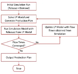
The Figure 3.1 below shows a flow chart of the HL iterative algorithm
procedure.
Figure 3.1: Flow chart of Iterative Algorithm of HL Procedure
In the next section we describe the clearing function model to which the results
of the Hung and Leachman model will be compared.
3.2.Allocated Clearing Function (ACF) Model
In this thesis, we use ACF formulation of (J. M. Asmundsson, Rardin, R. L.,
Uzsoy, R., 2002) since we have multiple products competing for production resources.
3.2.1.LP Formulation
We define the following notation:
g : product type index.
k : machine index.
l : operation index.
Dgp : demand for wafer type g during period p.
Ygpl : product quantity consuming machine hours at operation l for wafer type g in
period p.
Ygpk : product quantity consuming machine hours at machine k for wafer type g in
period p. Summation of all Ygpl in machine k gives Ygpk.
Xgpl : product release quantity for product type g in period p at operation l.
Xgpk : product release quantity for product type g in period p at machine k.
Summation of all Xgpl in machine k gives Xgpk.
Ygp : product output quantity for product type g in period p.
Xgp : product release quantity for product type g in period p.
Wgpk : WIP of product type g during period p at machine k. Summation of all Wgpl in
machine k gives Wgpk.
: Fraction of capacity at machine k in period p, allocated to product type g.
C(k) : set of indices denoting the line segments used at machine k.
µ : Intercept of clearing function of segment n, machine k.
: Slope of clearing function of segment n, machine k.
Decision Variables:
Xgp : product release quantity for product type g in period p.
Igp : units of product g in finished goods inventory at the end of period p.
Bgp : units of product g backlogged at the end of period p.
Parameters:
hgp : Unit inventory holding cost for product g in period p.
bgp : Unit backlogging cost for product g in period p.
Objective function:
∑ ∈ ∑ ∑ ω + + ∑ ∈ ∑ ℎ + ∑ ∈ ∑
(3.12)
Subject to:
= , , + − ∈ , = 1, … , , l ∈ (3.13)
+ , − , − + = ∈ , = 1, … , (3.14)
≤ µ + + , , ∈ , = 1, … , , ∈ K, ∈ C(k) (3.15)
∑ ∈ = 1 = 1, … , , ∈ K (3.16)
, , , , , ≥ 0 ∈ , = 1, … , , ∈ K (3.17)
This formulation uses variables to allocate capacity among products. These
variables scale up the summation of WIP of product g at the beginning of period p and
releases within the period p of product g to obtain the upper bound of the output of
product g at machine k. Equation (3.15) can operate to determine the fractional total
capacity to product g. The development of this formulation is given in (J. M.
Asmundsson, Rardin, R. L., Uzsoy, R., 2002).
It is important to note that a separate clearing function is formed for each
machine in the production system. The Allocated Clearing Function model takes the
based on WIP at the beginning of the period and releases within the period and the
shape of the clearing function.
In the following chapter we will talk about our experimental design, the
simulation model that we use, the steps of fitting clearing functions and our
CHAPTER 4. EXPERIMENTAL
DESIGN
The two LP models that we compare use the output of our simulation model as
inputs. HL procedures combines LP with simulation for passing information between
iterations. Allocated Clearing Function model requires data to fit clearing function
which will be obtained from long run simulation. We will give description and
characteristics of our simulation model and then continue with the fitting of clearing
functions.
4.1.Simulation Model
Our simulation model of a re-entrant bottleneck system was built with
attributes of a real-world fab environment, studied by Uzsoy in previous research
(Kayton, Teyner, Schwartz, & Uzsoy, 1997). The major characteristics of wafer
fabrication, including a re-entrant bottleneck process, unreliable machines, batching
machines and multiple products with varying process routings and number of
operations were included in the model. There is a distinct re-entrant bottleneck
machine representing the photolithography process. The processing times for all other
stations were scaled to the bottleneck processing time so that no non-bottleneck station
would have a utilization approaching that of the bottleneck. The model has batching
stations (Stations 1 and 2) early in the process, representing the furnaces which
two lots and the maximum batch size is four lots. The batching stations can be loaded
with any product lot mix, that is, a batching station can run lots of one type of product
or many product types at one time. The remaining stations process one lot at a time.
Figure 4.1: Re-entrant Bottleneck Model Process Chart for Products
There are 11 machines (stations) and 3 products in this model. The number of
operations for product 1, product 2 and product 3 are 22, 14 and 14 respectively.
Machine 4 is the re-entrant bottleneck machine shown as red in Figure 4.1. There are
two servers in machine 4. Product 1 and product 2 visit bottleneck machine 6 times
and 4 times respectively. Product 3 does not use bottleneck machine. This product
visits Station 11 which is the only station that is allowed to exceed 80% utilization, but
it is not allowed to exceed the bottleneck utilization. There are 2 batching machines,
process. There are 2 unreliable machines, machine 3 and machine 7, shown as black in
Figure 4.1. These unreliable machines cause starvation at the bottleneck machine. The
system is required to produce a product mix that is 3:1:1 of Product 1, 2, and 3
respectively.
4.1.1.Simulation Parameters
The distributions of processing times and failures and their parameters will be
presented in this section.
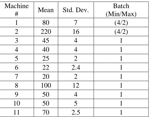
4.1.1.1.Simulation Processing Times
Table 4.1: Simulation Processing Times and Batch Sizes
Machine
# Mean Std. Dev.
Batch (Min/Max)
1 80 7 (4/2)
2 220 16 (4/2)
3 45 4 1
4 40 4 1
5 25 2 1
6 22 2.4 1
7 20 2 1
8 100 12 1
9 50 4 1
10 50 5 1
11 70 2.5 1
All processing times follow a lognormal distribution. The processing times are
percent of the mean. The processing times for all individual products in a machine are
same. Also, the processing time of a machine for different operations is same.
4.1.1.2.Failure Distribution Parameters
Table 4.2: Failure Distribution Parameters
MTTF MTTR
Machine
# Alpha Beta Mean
Std.
Dev. Alpha Beta Mean
Std. Dev.
3 7200 1 7200 83.7 1200 1.5 1800 52
7 7200 1 7200 83.7 1200 1.5 1800 52
The mean time to failure (MTTF) and mean time to repair (MTTR)
distributions follow gamma distributions. Machines 3 and 7 are the unreliable
machines can produce a product in a very short time but can starve the bottleneck due
to poor availability. The mean and standard deviations values are calculated from
input analyzer of Arena Version 10.0 (www.arenasimulation.com). A Sample of 5000
data points is created given the alpha and beta values. Sample mean and standard
deviations are found as given in the Table 4.2. The values are in minutes. Availability
can be calculated as follows,.
=
. , % (4.1)
This can be interpreted as on average machines are operating 80% of the time.
4.1.1.Simulation Details
The simulation model is created in Arena version 10.0 (www.arenasimulation
.com) that runs on a Intel PC with a Intel(R) Core(TM) 2 CPU 6700 2.66 GHz
processor and 2GB of RAM, under Microsoft Windows XP Professional.
The period length for the production planning models is 7 days. The
simulation is run for 26 periods. 5 replications are done for each simulation. The
release entities are created daily, at the beginning of the day, by reading the data from
an Excel file. The transfer of release inputs to simulation will be discussed in Section
4.3. After the products are released to the system before their first operation, the
products are lined up in the order of products 1,2 and 3 repeatedly. The excess
amounts of products are put in front of other products following the same ordering
logic. We use this procedure to have more uniform output rates and flow time
estimates of the products. Lots are dispatched in First-in-First-Out order on all
machines.
After presenting our simulation model, we will discuss our LP models in the
next section.
4.2.LP Models
In our experiments the LP models are implemented in the OPL Version 5.5
PC with a Intel(R) Core(TM) 2 CPU 6700 2.66 GHz processor and 2GB of RAM,
under Microsoft Windows XP Professional.
We have two LP models that we will discuss and compare in this study. The
details in the execution of these LP models will be explained below.
4.2.1.Hung and Leachman Iterative Algorithm
In this model we use simulation to estimate our flow times and do iterations.
At each simulation run, we do replications to have good estimates of flow times. The
number of simulation replications is selected based on a tradeoff between the need to
obtain some statistical precision in our estimates of the flow times, while keeping the
computational burden of the overall iterative procedure within reasonable limits. We
select the number of iterations as 10 for the reasons described above.
In the original work, Hung and Leachman require the Mean Absolute
Deviation of the average flow time across all products to be within 5% from one
iteration to the next, but this leaves open the possibility of fluctuations in the flow
times of each product that cancel out across products and also can cause significant
differences in the realized output. A more stringent criterion would be to require the
Mean Absolute Deviation (MAD) of flow times for all individual products to be below
some tolerance. A less demanding approach would require the objective function
criterion bases on the results that we obtain and they will be presented in the
experimental results section.
As we describe in Section 3.1, the HL procedure requires flow time estimates
Fglp at the end of each period. In the simulation model, the flow times of all individual
products for all operations are written to an Excel file with Visual Basic Scripts. The
data is then filtered and sorted to estimate the flow times at specified points which are
called epochs. In the HL model epoch points are the beginning of each period. The
flows times immediately before and immediately after the epoch are found and they
are interpolated to get the estimate at the epoch. This is done for all operations,
products and periods. These flow time estimates are fed to OPL studio and the new
optimum release schedule is obtained using these flow time estimates. This release
schedule is sent to Arena Software to get the new flow time estimates for the given
release schedule. The communication between Arena Software and OPL Studio is
established by Visual Basic. The information passing in the iterations between LP and
Simulation is done by number of Visual Basic scripts. The detailed steps of HL
procedure are described in Section 3.1.2.
The LP model is applied to 26 Periods and cost and revenue values that are
Table 4.3: Cost and Revenue Values
inventory cost
Backlog cost
Material
cost Revenue
15 50 3 60
These values are per unit product and same for all three product types. These
costs and revenue value can be interpreted as relative to each other. In our study, we
use backlog cost much higher than inventory holding cost but slightly less than
revenue. We want to push our model to favor satisfying demand instead of holding
backlog. The release cost value which is the material cost, is much more less than
others, but shows releasing still has some cost.
4.2.2.Allocated Clearing Function (ACF) Model
In the ACF model, our main focus is to fit a clearing function and implement it
in an LP model. We need the intercept and slope values of the clearing function for
each segments. In this study we use three segments as will be further explained in
Section 4.4.
The ACF model also finds the optimal production planning for 26 periods and
the associated cost values are shown in the table below.
Table 4.4: Cost Values of ACF Model
Inventory cost
WIP cost
These cost values can be interpreted as relative, i.e., that holding WIP in the
factory is more than twice as much as holding finished goods inventory. We try to
push the model to find optimum production plan without holding WIP in the factory.
The cost of holding WIP can also be interpreted as, holding WIP in front of machines
instead of holding finished goods inventory is much higher due to the limited space in
the factory.
In this model, the inventory levels for all products at the beginning of the
planning model are initialized to average demand of products to mediate the output LP
and simulation differences in the first planning period that will be explained in
Chapter 5.
4.3.Conversion of LP Releases to Simulation Input
In our study, we compare the desired output at the objective function value
predicted by the LP models, with the outputs obtained from Simulation using the
release schedule as a performance criterion. The details will be explained in the
performance criterion section.
The release schedule that is found by LP models may be fractional instead of
integer numbers. Simulation requires integer values for the releases so in order to give
the release schedule suggested by LP as an input to Simulation, the fractional values
In addition to the issue explained in the previous paragraph, the release
schedules suggested by the LPs are weekly release schedules. Our period length is one
week. In our simulations, we assume that the releases of a period are uniformly
distributed over that period. In order to achieve that, we convert the weekly release
schedules to daily release schedules of that period.
In order to address these fractional value and uniform distribution of release
problems, we use an algorithm that rounds some values up and some values down. We
do not simply round up all values since the cumulative effect would be high in this
case. In our algorithm, we divide the release schedule of one period, that is one week
in our study, into equal daily release schedules. This is simply done by dividing the
weekly schedule by seven for all periods. Then, the release of first day of that period is
always rounded up. The difference between actual fractional releases and rounded
releases are recorded. If the cumulative difference is greater than 0.001 , the next value
is rounded down,. If the cumulative difference is less than 0.001, then the next value is
rounded up. In this case, the difference between cumulative release schedule of the
planning horizon from LP and cumulative adjusted release schedule for simulation
input is close to zero. Thus, LP release schedules and Simulation input schedules are
matched closely enabling us to compare LP outputs to simulation outputs more
Step 1: Divide the weekly schedule into equal daily schedules by dividing the
release schedule from LP by seven.
Step 2: Round up the first release day of that period.
Step 3: Check whether cumulative differences of actual releases from LP and
rounded releases are greater than 0.001 or not. If the quantity is greater, round down
the corresponding fractional release. If it is less than 0.001, than round up the
corresponding fractional release. Go to next daily schedule.
Step 4: When the calculations are done for one weekly schedule, start over the
process with the next weekly schedule, following the steps 1, 2 and 3.
4.4.Fitting Clearing Function
For the Allocated Clearing Model, we need to fit a clearing function to be used
in the constraint equation (3.15). To achieve that first we collect data and then by
examining the data we investigate type of function to fit the data.
4.4.1.Data Collection for Fitting
In this study, we investigate the clearing function form where output is a
function of releases within the period and WIP at the beginning of the period. The
function is given below.
Xit represents the total output of machine i at period t. Wi,t-1 represents the total
WIP at beginning of the period of machine i and Rit represents the total number of
releases within the period t of machine i. This function does not distinguish between
products, but deals with total numbers in a period. We explain in Section 3.2.1, how
the allocation of capacity is handled by variable to individual products.
As described in the previous paragraph, the data needed to fit a function for
each machine is Rit, the total releases within a period, Wi,t-1 total number of WIP at the
beginning of the period and Xit ,total number of outputs in that period.
4.4.1.1. Outline for Data Collection
In the previous section, we identify the type of data that we require to fit the
clearing function. We follow the steps below to obtain sufficient data to fit our
clearing function.
Step 1: Seven different release schedules of 91 periods from normal
distribution are created corresponding to bottleneck utilization of around 49%, 60%,
70%, 77%, 87%, 94% and 99%.
Step 2: For each schedule, Simulation is run for 91 periods with five
replications, collecting the data Xit, Rit and Wi,t-1 required for each machine.
Using the simulation model and parameters explained in Section 4.1, the
following plots are obtained. The plots show output as a function of releases within a
period plus WIP at the beginning of that period. We will refer releases within a period
plus WIP at the beginning of that period as resource load.
4.4.1.2.Plots of Empirical Data for Selected Machines
We have eleven machines in our system. For the sake of brevity we include the
most interesting machines: machine 1 which is the first operation machine for all
products, and a batching machine, machines 3 and 7 which are the unreliable
machines, and machine 4 which is the bottleneck machine. The plots of other
machines are straightforward having a linear accumulation of data without much
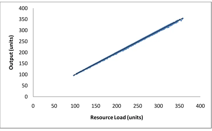
Figure 4.2: Machine 1 Output vs. Resource Load
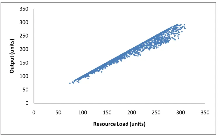
Figure 4.3: Machine 3 Output vs. Resource Load
0 50 100 150 200 250 300 350 400
0 50 100 150 200 250 300 350 400
O
ut
pu
t (
un
its
)
Resource Load (units)
0 20 40 60 80 100 120 140 160
0 50 100 150 200
O
ut
pu
t (
U
ni
ts
)
Figure 4.4: Machine 7 Output vs. Resource Load
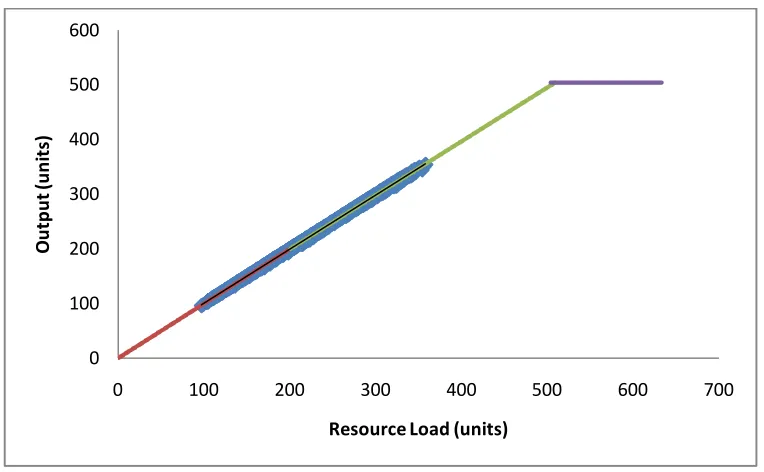
Figure 4.5: Machine 4 Output vs. Resource Load
0 50 100 150 200 250 300 350
0 50 100 150 200 250 300 350
O
ut
pu
t (
un
its
)
Resource Load (units)
0 100 200 300 400 500 600
0 200 400 600 800 1000 1200
O
ut
pu
t (
un
its
)
Figure 4.2 show the plot of machine 1 which is the one of the batching
machines. We observe a linear relation between output and resource load. Figure 4.3
shows the plot of Machine 3 which is an unreliable machine. On this plot we also
observe a linear relation between output and resource load since the data is mostly
accumulated on the linear line having deviations due to failure. Figure 4.4 shows the
plot of machine 7, another unreliable machine. It behaves very similar to plot of
machine 3 for the same reasons mentioned for machine 3. Figure 4.5 shows the plot
of machine 4 which is our bottleneck machine. On this plot we observe that there is
good linear relation until it reaches to its capacity value. After some point the line
becomes horizontal since the machine reaches its capacity and increasing resource
load does not increase the number of outputs.
The plots of other machines are very similar to the plot of machine 1 shown in
Figure 4.2. We observe good linear relation between output and resource load for
these machines. After observing the plots, we will talk about fitting our linear
functions to different segments in the next section.
4.4.2. Fitting Clearing Function to Data
We observe from the plots that there is a piecewise linear relation between
outputs and summation of release and initial WIP. We apply simple linear regression
the capacity limit of the machines which will be estimated by dividing the period
length by the mean process times of the machines given in Table 4.1. For machines 3
and 7, due to presence of machine failure we take into consideration availability in the
period meaning that after dividing the period length by the mean process times, we
also multiply it by the availability to have a better estimate of capacity limit. The first
and the second segments will include the estimation of intercept and the slope values
of the linear section by splitting the linear section into two parts. To do this, we find
the range of the linear section by finding the minimum and maximum summation of
release and initial WIP. We calculate 40% of the range and add it to minimum
summation value. This becomes the upper bound of the first section. In the first
segment we fit the data between minimum summation value and the upper bound of
the first section. The upper bound of the first section becomes the lower bound of the
second section. In the second section we fit the data between lower bound of the
second section and maximum summation value. The reason of dividing the linear part
into two segments is to capture any change of slope or intercept values when the
machine gets closer to its capacity limit instead of using one line which would give
less accurate estimates.
Using the procedure described in the previous paragraph we get the following
Figure 4.6 : Machine 1 Linear Regression Fit
Figure 4.7: Machine 3 Linear Regression Fit
0 100 200 300 400 500 600
0 100 200 300 400 500 600 700
O
ut
pu
t (
un
its
)
Resource Load (units)
0 20 40 60 80 100 120 140 160 180 200
0 50 100 150 200 250 300 350
O
ut
pu
t (
U
ni
ts
)
Figure 4.8: Machine 7 Linear Regression Fit
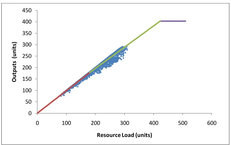
Figure 4.9: Machine 4 Linear Regression Fit
0 50 100 150 200 250 300 350 400 450
0 100 200 300 400 500 600
O
ut
pu
ts
(
un
its
)
Resource Load (units)
0 100 200 300 400 500 600
0 200 400 600 800 1000 1200
O
ut
pu
t (
un
its
)
In these graphs, blue dots show the actual data. The red line shows the fitted
linear regression line of the first segment. The green line shows the fitted linear
regression line of the second segment. The purple line shows the capacity limit line
where slope is equal to zero and intercept is equal to period length divided by mean
process time. The statistics of the fitted linear regression lines is given in the table
below.
Table 4.5: Statistics of Fitted Linear Regression Lines
Segment 1 Segment 2 Segment 3
Intercept Slope R2
value Intercept Slope
R2
value intercept Slope Machine1 0.13 0.9948 0.9974 1.50 0.9877 0.9985 504.0 0 Machine3 1.06 0.9683 0.9426 18.93 0.7913 0.7543 179.2 0 Machine7 0.24 0.9852 0.9647 11.26 0.9260 0.9365 403.2 0 Machine4 0.64 0.9933 0.9977 26.21 0.9171 0.9877 504.0 0
We observe from the fitted linear regression lines that they have high R2 values
above 93% except machine 3, which its second segment has 75%. High R2 values
imply that the fitted lines can explain the variability of data well. From the figures we
can observe that the fitted lines represent the data quite well. For the machine 3, due to
failure there are deviations from the fitted line however it still has R2 value of 75%
that the line has strength to explain the variability of 75% of the data. Although
machine 7 is also failure machine, it does not get affected by failures as much as
From the figures we see that only machine 4 has the data that follows our third
segment line. The reason is that, machine 4 is the bottleneck machine that has the
highest utilization in the system. We can collect data of the segment for the machine 4
that represents the capacity limit. Other machines do not reach their capacity limits so
we do not observe any data around the capacity limits for them.
The plots are drawn and estimation of clearing functions are done using the
seven schedules. Now the question is if we use a different set of seven schedules, will
we have same plots and estimation of clearing functions? We answer this question in
the next section.
4.4.3.Does the Clearing Function depend on other schedules?
As we describe in Section 4.4.1.1, we collect the empirical data with seven
different schedules that come from normal distribution and we fit the regression lines
to this empirical data, thus obtain intercept and slope values for each machine. We
show the results in Section 4.4.1.2. We ask the question if we change the seven
schedules having the respective utilizations that we used in forming the data, does the
clearing function change?
To address this question we follow the steps below
Step 1: Take the previous seven release schedules and implement them as
and slope values from the first clearing function, solve LP to get new seven release
schedules.
Step 2: For each schedule, simulation is run for 91 periods with five
replications, collecting the data needed for each machine.
Step 3: All the data is combined to one file and plotted for each machine.
Step 4: Fit linear regression line and find the intercept and slope values for
each sections.
We will compare intercept and slope of each segment for all machines for both
clearing functions that we use different set of seven schedules.
In addition to the procedure that described above, we use the HL procedure
with one iteration of five replications to estimate the flow times, giving the original
seven schedules as starting release and demand variables. Thus we get new set of
seven schedules. We apply the same steps starting from step 2, and get another set of
clearing functions. We obtain the following comparisons in the figure below. We
name our original clearing function as CF1, our second clearing function as CF2 and
Figure 4.10: Intercept Comparison of Segment 1
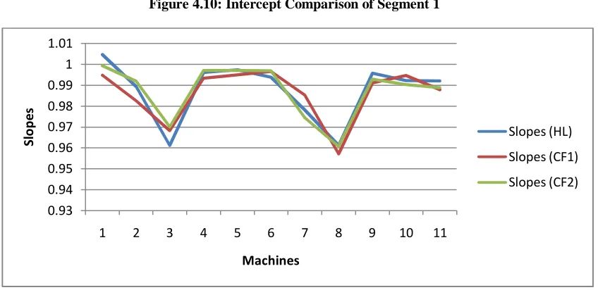
Figure 4.11: Slope Comparison of Segment 1
-1.5 -1 -0.5 0 0.5 1 1.5 2
1 2 3 4 5 6 7 8 9 10 11
In
te
rc
ep
ts
Machines
intercept HL intercept CF1 intercept CF2
0.93 0.94 0.95 0.96 0.97 0.98 0.99 1 1.01
1 2 3 4 5 6 7 8 9 10 11
Sl
op
es
Machines
Figure 4.12: Intercept Comparison of Segment 2
Figure 4.13: Slope Comparison of Segment 2
From the plots, we can observe that changing the release schedule using
different LP models does not make much difference in the clearing function itself.
When we look at the slopes, the values from CF1, CF2 and HL are quite close to each
other. In terms of Intercepts, the values from CF1, CF2 and HL are also close to each
-10 0 10 20 30 40
1 2 3 4 5 6 7 8 9 10 11
In
te
rc
ep
t
Machines
intercept (HL) Intercept (CF1) Intercept (CF2)
0.7 0.75 0.8 0.85 0.9 0.95 1 1.05
1 2 3 4 5 6 7 8 9 10 11
Sl
op
es
Machines
other but not as much as the slope values; however the differences do not significantly
change the overall shape of the clearing function.
In summary, changing the data collection methods to form the clearing
function by using other LP models, does not change the shape of the clearing function
itself.
In the next section we will talk about our experimental factors that we will use
as a testbed when we compare the performance of our LP models.
4.5. Experimental Factors
In our study, our experiments were designed to examine the effects of two
different factors on the performance of the HL procedure and Allocated Clearing
Function model. The factors are bottleneck utilization with different demand patterns
and the length of mean time to failure (MTTF) and mean time to repair (MTTR).
4.5.1.Bottleneck Utilization with Different Demand Patterns
It is well known from queueing theory that the nonlinear relationship between
resource utilization and flow times becomes more severe at high utilization levels.
Hence one would expect an LP model using fixed, exogenous flow time estimates to
perform well at low utilization levels, but to degrade in performance at higher
utilization. We aim to observe these effects in HL procedure. Also, for Allocated
more important to be able to address the relation between output and summation of
release and initial WIP. We aim to observe how our linear clearing function fits
perform at high utilizations. Hence we experiment with two bottleneck utilization
values of 0.7 and 0.9. The utilization level is achieved by varying the demand of all
products while maintaining the 3:1:1 product mix. We also consider two different
demand patterns. One is constant demand pattern which stays constant throughout the
planning horizon of 26 periods. We aim to test our algorithms under favorable
conditions. Second case is varying demand pattern which the demand changes from
period to period. We aim to test how our algorithms will perform under varying
demand. In the next section we present our demand patterns that we will use to test the
performance of the LP models.
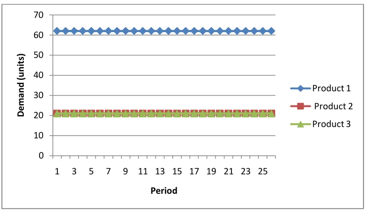
4.5.1.1.Constant Demand Pattern
We have two cases. First case is constant demand pattern that will give
approximately 70% bottleneck machine utilization. And second case is constant
demand pattern that will give approximately 90% bottleneck machine utilization.
Product mix 3:1:1 for product 1, product 2 and product 3 is maintained. The figures
Figure 4.14: Constant Demand Pattern corresponding 90% Utilization
Figure 4.15 Constant Demand Pattern corresponding 70% Utilization
0 10 20 30 40 50 60 70
1 3 5 7 9 11 13 15 17 19 21 23 25
De m an d (u ni ts ) Period Product 1 Product 2 Product 3 0 10 20 30 40 50 60
1 3 5 7 9 11 13 15 17 19 21 23 25
4.5.1.2.Varying Demand Patterns
In this case, we have varying demand pattern where the demand changes over
time. The first and last three periods demands are set constant in order to minimize
beginning and ending effects. Again we have two varying demand patterns that will
give 90% and 70% bottleneck utilization. The figures below show these demand
patterns.
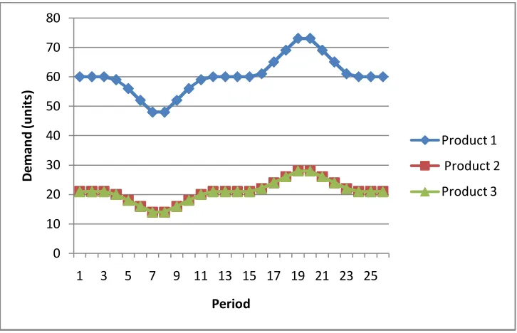
Figure 4.16: Varying Demand Pattern corresponding 90% Utilization
0 10 20 30 40 50 60 70 80
1 3 5 7 9 11 13 15 17 19 21 23 25
De
m
an
d
(u
ni
ts
)
Period
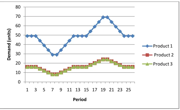
Figure 4.17: Varying Demand Pattern corresponding 70% Utilization
In the next section we present two cases of length of MTTF and MTTR. We
will name original MTTF and MTTR parameterized simulation model as short failure
case. We will have twice as much as these MTTF and MTTR parameterized models
which we will call long failure case.
4.5.2.Length of MTTF and MTTR
We will consider two cases. In the first case is that we use the original
parameters of MTTF and MTTR that are given in Table 4.2: Failure Distribution
Parameters. We will refer this case as the short failure case. Our second case will be
failures with longer MTTF and MTTR times for both failure machines. We will refer
to this case as the long failure case.
0 10 20 30 40 50 60 70 80
1 3 5 7 9 11 13 15 17 19 21 23 25
De
m
an
d
(u
ni
ts
)
Period
We aim to test how the flow time estimates will be affected by longer MTTF
and MTTR values and how this will change the optimum solution of the LP. We also
aim to see how the fitting of the clearing function will change due to this new
condition since we change the system so we expect changes in clearing functions for
all machines.
4.5.2.1.Short Failure Case
In this case, we use the original values of MTTF and MTTR, with
MTTF = 7200 minutes and MTTR = 1800 minutes. Our period length is 10080
minutes meaning that on average the machines will fail once in every period. The
corresponding empirical data and fitted clearing functions are given in Sections 4.4.1
and 4.4.2.
4.5.2.2.Long Failure Case
In this case, we aim to have longer MTTF and MTTR keeping the availability
same as in the short failure case. We decide to double the MTTF and MTTR values so
in order to achieve that we multiply alpha parameters of gamma distribution by 2. We
Table 4.6: Failure Distribution Parameters for Long Failure
MTTF MTTR
Machine
# Alpha Beta Mean
Std.
Dev. Alpha Beta Mean
Std. Dev. 3 14400 1 14400 118 2400 1.5 3600 72.2 7 14400 1 14400 118 2400 1.5 3600 72.2
MTTF and MTTR values are twice those the short failure version. The period
length is 10080 minutes so it is possible that we don’t have any failures in each period
but once there is failure it will take more than one third of a period. We expect to see
these effects in our clearing function. We will present machines 1,3,7 and 4 in order to
show the effects. The empirical data plot for these machines are given below.
Figure 4.18: Machine 1 Output vs. Resource Load for Long Failure
0 50 100 150 200 250 300 350 400 450
0 100 200 300 400 500
O
ut
pu
t (
un
its
)
Figure 4.19: Machine 3 Output vs. Resource Load for Long Failure
Figure 4.20: Machine 7 Output vs. Resource Load for Long Failure
0 20 40 60 80 100 120 140 160 180 200
0 50 100 150 200
O ut pu t ( U ni ts )
Resource Load (units)
0 50 100 150 200 250 300 350 400
0 50 100 150 200 250 300 350 400
O ut pu t ( un its )