Experimental and Computational Studies of Gravity-Driven Dense Granular Flows.

(1)

ABSTRACT

CHILAMKURTI, YESASWI NARENDRA. Experimental and Computational Studies of Gravity-Driven Dense Granular Flows. (Under the direction of Richard Gould).

The current work focusses on the characterization of gravity-driven dry granular flows

in cylindrical tubes. With a motive of using dense particulate media as heat transfer fluids

(HTF), the study was primarily focused to address the characteristics of flow regimes with a

packing fraction of ~60%. Experiments were conducted to understand the effects of different

flow parameters, including: tube radius, tube inclination, tube length and exit diameter. These

studies were conducted on two types of spherical particles – glass and ceramic – with mean

diameters of 150 µm and 300 µm respectively. The experimental data was correlated with the

semi-empirical equation based on Beverloo’s law. In addition, the same flow configuration

was studied through three-dimensional computer simulations by implementing the Discrete

Element Method for the Lagrangian modelling of particles. A soft-particle formulation was

used with Hertz-Mindilin contact models to resolve the interaction forces between particles.

The simulation results were used to examine the velocity, shear rate and packing fraction

profiles to study the detailed flow dynamics. Curve-fits were developed for the mean velocity

profiles which could be used in developing hydrodynamic analogies for granular flows. In

addition, the particle-wall contact behavior was also studied to characterize the heat transfer

from the wall to the granular flow. Finally, the fluctuations inside the flow were also studied

using computer simulations and their dependency on the tube length was characterized. Thus

the basic features of gravity driven dense granular flows were identified to form a basis for

(2)

(3)

Experimental and Computational Studies of Gravity-Driven Dense Granular Flows

by

Yesaswi Narendra Chilamkurti

A thesis submitted to the Graduate Faculty of North Carolina State University

in partial fulfillment of the requirements for the degree of

Master of Science

Mechanical Engineering

Raleigh, North Carolina 2016

APPROVED BY:

______________________________ Richard Gould

(4)

DEDICATION

(5)

BIOGRAPHY

The author was born on the 18th of May, 1992 in Gudlavelleru, in the state of Andhra Pradesh,

India. He received his Bachelor’s degree in Mechanical Engineering from Indian Institute of

Technology Patna (IIT Patna) in May 2013. The author went on to study Mechanical

Engineering in North Carolina State University (NCSU), Raleigh, North Carolina in fall 2013.

Here, he began working in the Heat Transfer Laboratory from January 2014. His academic and

(6)

ACKNOWLEDGMENTS

I would first like to thank my advisor Dr. Richard Gould for his great support and help with

my research work in the past two years at North Carolina State University. I would also like to

thank my committee members Dr. Tarek Echekki and Dr. Alexei V. Saveliev for their valuable

time. I would like to thank my lab mates Megan Watkins and Alexander Szersen for their

assistance and encouragement with my research work. I would also like to express my gratitude

to ARPA-E (Advanced Research Projects Agency-Energy) for the financial support they

provided throughout my tenure. Furthermore, I would also like to thank the folks at RTI

International for their valuable suggestions and inputs that guided my research direction over

the past two years.

I would genuinely and sincerely like to thank my close friends Bharadwaj, Sandeep, Praveen,

Pallavi, Sneha, Vishnu, Avinash, Nadish, Hari and Manu who, without their own knowledge,

helped me in coping up with my low times and gave me some of the best moments I can cherish

throughout my life. Finally and most importantly, I would like to thank my parents whose love

and moral support instilled in me the confidence to face the challenges of life and who continue

(7)

LIST OF TABLES

(10)

LIST OF FIGURES

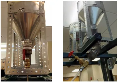
Figure 2.1 Funnel assembly in the experimental setup ... 7

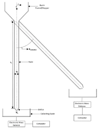
Figure 2.2 Overall Experimental setup for vertical tube and inclined tube (left to right)8 Figure 2.3 Schematic of the experimental setup ... 9

Figure 3.1 Flow through the transparent tube resembling a continuum fluid ... 13

Figure 3.2 Variation of mass flow rates with orifice diameter ... 14

Figure 3.3 Flow behavior for different tube lengths and inclinations ... 17

Figure 4.1 Particle contact force formulation on the contact plane ... 21

Figure 4.2 Particle injection into the solution domain using lattice structures ... 27

Figure 4.3 Simulation geometry without and with particles (left to right) ... 29

Figure 4.4 (clockwise) (i) SEM image of particulate sample at 10X magnification (ii) SEM image of particulate sample at 50X magnification (iii) Energy spectrum of the particulate sample at position S1 ... 30

Figure 4.5 Methodology used to calculate the angle of repose using simulations ... 33

Figure 5.1 Validation of flow rates obtained in the Discrete Element simulations ... 37

Figure 5.2 Contour plots of particulate velocities (a) through the orifice (b) through a flow cross-section ... 38

Figure 5.3 Sectioning of flow cross-section into annular rings for boundary sampling 40 Figure 5.4 Time evolution of particulate velocities at different radial locations ... 41

Figure 5.5 Time averaged particulate velocity at 3.5g/s mass flow rate (tube diameter: 0.007747m and particle diameter: 300 microns) ... 42

Figure 5.6 Gaussian fit for time-averaged particulate velocity at 3.5g/s flow rate (tube diameter: 0.007747m and particle diameter: 300 microns) ... 45

(11)

Figure 5.8 Radial profiles of axial velocity for different flow rates for 0.010922m tube diameter (mass fluxes vary from 74.2kg/m2_{-s g/s to 281.4kg/m}2_{-s) ... 47} Figure 5.9 Variation of slip and maximum velocity with mass fluxes ... 48

Figure 5.10 Normalized mean axial velocity profiles for different flow rates in 0.005m diameter tube (mass fluxes vary from 35.7kg/m2_{-s g/s to 336.6kg/m}2_{-s) ... 49} Figure 5.11 Radial profiles of axial velocity for different mass fluxes with 475 micron particles and 0.007747m tube diameter (mass fluxes vary from 6kg/m2_{-s g/s to}

300kg/m2_{-s)... 51} Figure 5.12 Radial profiles of axial velocity for different mass fluxes with 600 micron particles and 0.007747m tube diameter (mass fluxes vary from 14kg/m2_{-s g/s to}

310kg/m2_{-s)... 52} Figure 5.13 Wall normal stresses versus axial position in tube of diameter 0.007747m for different flow rates. ... 54 Figure 5.14 Wall shear stresses versus axial position in tube of diameter 0.007747m for different flow rates. ... 56 Figure 5.15 Variation of effective friction with inertial number for different simulation cases ... 58 Figure 5.16 Packing fraction profiles for different flow rates for 0.007747m tube

diameter ... 59 Figure 5.17 Radial profiles of packing fraction for different flow rates for 0.010922m tube diameter ... 60 Figure 5.18 Variation of mass flow rates with orifice diameters for different tube

diameters ... 62 Figure 5.19 Variation of mass flow rates with orifice diameter for different particle sizes ... 63 Figure 5.20 Variation of particle-wall contact behavior with different particle

(12)

Figure 5.23 Propagation of density waves in 0.3m long tube shown in contour plots of particulate velocities and scalar plots of center-line velocities (Solution time increases with a time-step size of 0.0025s from left to right) ... 69 Figure 5.24 Density wave structure depicted using contour plots of particulate

(13)

Chapter 1

Introduction

With the increasing attention on using granular flows as a potential high temperature heat

transfer fluid [1]–[3], a careful study of the flow physics is required before implementing them

on an industrial scale. Use of flowing rigid particles, as opposed to the current heat transfer

fluids like steam and molten salts, could increase the working temperature range of the heat

transfer systems and open new opportunities for higher efficiency thermodynamic cycles.

Thus, applications that rely on direct/indirect absorption of heat energy, for example

concentrated solar power (CSP), may use dry particles for heat transfer and thermal storage

[4].

Though direct absorption systems are relatively easy to operate (and have high heat flux

density in case of CSPs), the convective losses and flow instabilities make it difficult to control

[5]. On the other hand, indirect heat absorption systems offer better control of particulate flows

making it preferable for industrial applications [6], [7]. Additionally, having dilute packing

fractions could result in poor thermal behavior owing to the interstitial gasses. As a result, the

current work primarily addresses the important characteristics of dense flow regimes in

(14)

From the study of static granular beds to the modelling of particulate collisions, our

understanding of granular physics has increased steadily [8]–[16]. With the help of high-speed

imagery and other non-intrusive techniques like PIV, X-ray, MRI, and ECT, several intrinsic

features were observed by the research community over the years. In addition, computational

methodologies like Molecular Dynamics and Discrete Element Analyses enabled the

investigation of these flows in an explicit manner. However, the flow characteristics vary from

configuration to configuration. In fact, every geometrical configuration has different flow

regimes, each of which having different governing physics. As a result, the most common

approach in understanding the flow rheology of granular media is by studying individual

configurations and extracting their intrinsic features.

The behavior of dense granular flows is highly sensitive to different geometrical

parameters, loading conditions and particle properties. Based on the particulate velocities,

granular flows are broadly divided into three types – quasi-static flows, dense flows and dilute

collisional flows. In the quasi-static regime, the inertia of individual particles becomes

negligible and the granular media behaves like a solid. This tightly packed regime (~ϕmax),

which is governed by particle properties like friction, elasticity, shape etc., can be modelled

using plasticity models of soil mechanics [11]. The dilute collisional regime, on the other hand,

is mainly governed by the inertia of the particles. This gas-like regime can be modelled using

analogies of the kinetic theory of gases [17] as the particles are strongly agitated and the

momentum transfer is mainly through collisions. Between these two, lies the dense collisional

flow regime which has a fluid-like rheology with non-negligible particulate inertia. Despite the

(15)

propagating the stresses layer by layer. All these regimes have different flow physics and as a

result, no universal framework was developed to describe the whole range from solid-like

quasi-static to gas-like collisional regimes. Hence, as mentioned earlier, the most convenient

way of describing granular flows is by studying individual regimes and individual

configurations and understanding their distinctive features separately.

Since we are currently interested in indirect heat absorption, the current work focuses on

confined granular flows that are primarily characterized by shearing at the boundaries. These

configurations can be represented by the non-dimensional inertial number 𝐼, which describes

the relative importance of particulate inertia to the confining stresses in granular flows. It is

the characteristic shear rate scaled by different time scales for different flow configurations

[16], [18], [19]. From the definition, an increasing inertial number indicates an increasing

deformation tendency of the particulate assemblies. In general, the granular flow lies in

quasi-static regimes for 0 < 𝐼 < 10−3 and in dense regimes for the ranges of 10−3< 𝐼 < 1. On the

other hand, the collisional regimes exist for 𝐼 > 1. Though these limits are not universal and

vary for different flow configurations, a qualitative understanding of the flow can be obtained

using these limits.

Typically, the heat transfer coefficients of granular heat transfer fluids (HTFs) increase

with increasing flow rates[1][20]. Similar trends are also observed with increasing packing

fractions within certain limits of temperature [7], [21]. As a result, the current work primarily

focusses on studies with higher packing fractions (60%) and relatively faster flows rates.

Conveying of particle suspensions can be achieved with both pneumatically driven measures

(16)

air voids and bubbles through the flow which would hinder the heat transfer phenomenon. As

a result, the current work primarily relies of gravity-driven configurations for achieving dense

flows.

Gravity driven flows have been studied over the years both experimentally and

computationally [16], [22]. But a majority of these studies focused on quasi-static or dilute

regimes. This is because most of the existing industrial applications and flow configurations

fall in these regimes. Though several researchers worked in the transitional dense regime, the

complexity associated with this regime has made its complete understanding a challenge [23].

Constitutive relations were developed to describe the stress-strain relations of this regime over

the years. But a universal model was never developed and each of them were specifically tuned

to their own flow/geometrical configurations. Moreover, observing dense configurations in

cylindrical tubes is another challenge. The opaque nature of the flow would make high speed

imaging techniques ineffective in studying the velocity and shear profiles. Unlike chute flows,

the opaque and three-dimensional nature of tube flows makes it difficult to analyze the internal

profile using flow visualization techniques. Though high speed visualization could be

attempted in a transparent tube, it would still be insufficient in predicting the internal flow

structure to analyze the velocity and shear profiles. In addition, non-intrusive techniques like

ECT, X-ray Imaging, etc. prove ineffective owing to the high packing fractions of the flow

[19]. Hence, the current research attempts to understand the different flow phenomena of the

dense flow regime in cylindrical tubes using both experimental and computational techniques.

A bench-scale experimental setup was developed to measure the room temperature

(17)

fraction inside the tube. Preliminary studies were conducted to analyze the influence of several

geometrical parameters of the flow. These results matched very well with those cited in the

literature [9] and also enabled the observation of several flow phenomena. Later, the

computational studies were conducted to observe the intrinsic features of the flow. The

particles were modeled with a Lagrangian approach by considering Discrete Element Methods

(DEM) [10]. Validated with the experimental results, the simulations studies helped us in

gaining further understanding of the internal flow rheology. In addition to flow characteristics

like velocity profiles, wall normal-shear stress profiles, flow rates and particle-wall contact

(18)

Chapter 2

Experimental Setup

The experimental setup was primarily designed to study the variation of flow rates with several

geometrical parameters. Though it did not give a clear understanding of the internal flow

configuration, the insights obtained from the experimental studies laid the foundation for the

entire research work. The following sections describes the experimental design, the

experimental methodology and the different cases studied.

2.1 Design

The experimental setup was designed to run in batches. Though conveyor setup was

initially planned to be installed to maintain a continuous flow, the current setup, being a

preliminary study was just designed in a simplistic manner. It includes a long vertical tube

with a flowrate controlling orifice at the bottom end. To maintain the batch-run configuration,

the setup was designed with a funnel at the top. The particles are fed into the funnel and they

flow into the pipe. Instead of using a flat-bottomed opening, a conical funnel was designed

with a divergence angle greater than the angle of repose of the particles (~26%). This was to

(19)

grade stainless steel and was erected vertically with four supports on the sides. The funnel

setup can be observed in figure 2.1. Since the tube diameters in the experiments were smaller

than the funnel exit, a flow reducer was attached.

Figure 2.1 Funnel assembly in the experimental setup

The flow reducer at the end of the funnel was attached to a flow control valve. The

cylindrical tube attached downstream of the valve with the help of compression fitting. The

experimental setup was also designed to understand the influence of tube’s inclination on the

flow. For that case, a 45o elbow fitting was attached to the exit of the funnel followed by a flow

reduced valve. The setup can be clearly observed in figure 2.1. The tubes are made of

stainless steel. Flow rates through the tube were controlled by creating a constriction at the end

(20)

of the tube using compression fitting. They act as a flow reducer at the exit and control the

particles flowing in the tube. They are also made of stainless steel. The overall experimental

setup can be observed in the figure 2.2. To make it rigid and sturdy, the entire setup was

mounted on a frame.

Figure 2.2 Overall Experimental setup for vertical tube and inclined tube (left to right)

2.2 Methodology

A single large quantity of granular material was loaded in the hopper (funnel) and the

experiment is carried on until the batch was complete. Before the experiment was started, the

(21)

tube completely. This was done to make sure that the flow configuration remained dense from

the initial stages of the experiment. Once the tube was filled, the orifice seal was removed and

the granular material started flowing. The entire flow process can be clearly understood from

the experimental schematic in figure 2.3.

(22)

Starting from the batch funnel/hopper the particles flow downward due to gravitational

force acting on them. These particles, which get slowed down at the orifice exit and leave the

tube, were collected in a basin that rests on an electronic mass scale (Adventurer™ Pro –

AV2102). This was connected to a computer and a temporal evolution of the mass flow rate

measurements were recorded throughout the experimental batch. Similar setup was also

adopted for the inclined tube experiments

Since the entire setup was just designed to measure the flow rates, another

mechanism/setup was needed to understand the flow pattern. The opaqueness of the stainless

steel tubes makes it difficult to observe the same. Hence another setup was also made with a

glass tube. The subsequent section gives details about the different experimental cases that

were performed in the study.

2.3 Run cases

As mentioned earlier, the experimental setup was designed to understand the influence of

different geometrical parameters on the flow rates. So, the different cases were run with

different orifice diameters, different tube lengths, different tube diameters and different tube

inclinations. Every experimental cases was run 5 times to avoid any errors in the obtained data.

Once the data is obtained, the mean values for each reading were used for further analysis.

Two tube diameters were considered in the experimental study. With a thickness of 0.9525

mm, inner diameters (𝐷𝑡) of 7.747 mm and 10.922 mm were used for the experimentation.

Each tube diameter was tested at three different heights (𝐿_𝑡). They are 1.82 m (6 feet), 1.22 m

(23)

conducted with a tube inclination of 45o from the horizontal. Each geometrical configuration

was tested with six orifice fixtures. The area ratios of these orifice fixtures, Aexit/Atube =

(Do/Dt)2, are 0.2, 0.25, 0.35, 0.5, 0.65 and 0.75. Preliminary experiments were conducted using

glass particles of 150 µm in diameters. But since, ceramic particles have good thermal

properties and they are the main pHTF (particle heat transfer fluid) that needed to be studied

in the research, further experimentation was done with them. The average diameters of these

ceramic particles was 270 µm.

The subsequent chapter includes the discussions about different observations that were

(24)

Chapter 3

Experimental Results

The following sections describe the different results obtained in the experiments and the

observations made from them. The first and foremost discussion is about the influence of

orifice diameter on the flow rates. Later observations about the influence of tube length, tube

diameter and tube inclination were discussed.

3.1 Variation of flow rates with orifice diameters

The flow rates remained constant throughout the experimental batch with very minor

fluctuations owing to the discrete nature of granular flows. Even though the height of the

particle bed in the funnel was decreasing with time, the flow rates remained constant

resembling a ‘choked’ flow at the tube exit. This contradicts to the observations one would

make in continuum flows. As a result, though the experiments were done in batches, it

remained like a steady state flow. From the observations made through the transparent glass

tubes, the flow looked steady and the particles moved at a constant speed. There was a sense

of intermittency in the flow that was negligible to observe. This could possibly be due to the

(25)

in the figure 3.1. It can be observed that the flow resembles a continuous flow with steady

stream of particle flowing out of the orifice.

Figure 3.1 Flow through the transparent tube resembling a continuum fluid

It was observed that with increasing orifice size, the flow rate increased. This was observed

for all the tube diameters, tube lengths and particle types. In figure 3.2, the variation of mass

flow rates with orifice diameter is plotted for different tube radii and particle types. It was

observed that the experimental data followed the semi-empirical Beverloo correlation [24] very

well. It is defined as:

𝑀̇ = 𝐶𝜌𝑏√𝑔(𝐷𝑜− 𝑘𝐷𝑝)5/2 (1)

It states that the mass flow rate 𝑀̇ of a free flowing granular material through a circular

(26)

the material 𝜌_𝑏, and the acceleration due to gravity 𝑔. In equation 1, 𝐶 and 𝑘 are the empirical

parameters that depend on the particle shape and friction[9]. This relation was obtained after

extensive studies done by several research communities over the years. It was suggested that a

free-fall dome is formed right about the exit of the orifice. It forms an arch shaped structure

that encloses the exit. Above the arch, the grain are well-packed and the velocities are less.

And on the other hand, below the arch, the particle accelerate freely under the influence of

gravity. The characteristic size of this free-fall arch/dome proportional to the diameter of the

orifice, 𝐷_𝑜. As a result, the velocity of the particles at the exit would be proportional to 𝐷_𝑜1/2

(Velocity of a free fall object from height H is √2𝑔𝐻). Hence the flow rate of particles is

proportional to 𝐷_𝑜5/2.

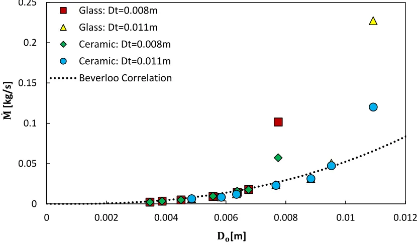
Figure 3.2 Variation of mass flow rates with orifice diameter

0 0.05 0.1 0.15 0.2 0.25

0 0.002 0.004 0.006 0.008 0.01 0.012

Glass: Dt=0.008m Glass: Dt=0.011m Ceramic: Dt=0.008m Ceramic: Dt=0.011m Beverloo Correlation

̇

𝐌

[kg

/s

]

(27)

From Figure 3.2, it can also be observed that for larger orifice diameters, the flow rates

suddenly increase to a high value and no longer follow the Beverloo Correlation curve. At this

point, it was also observed that the granular flow loses the continuum nature inside the tube.

The particle flowrates measured from the mass scales fluctuated with large magnitudes. In

addition, when observed using the transparent tubes, the flow started to have air spaces and

voids propagating through them. Thus, at Do = 7 mm and 10 mm for the 8 mm and 11m m tube

diameters respectively, there is a transition from dense flows to dilute flows inside the tube

with a “un-choking” phenomenon at the orifice. The take-off point at which the transition

occurs is different for different tube diameters but similar for both the types of particles. Similar

observations were made in other works [25], [26]. It was suggested by Huang et al. that the

free-fall arch at the orifice usually dissipates the kinetic energy of oncoming particles and slow

them down. It is then, these particles which undergo a free-fall and follow the

Beverloo-correlation. But if the kinetic energy of the granular media increases beyond a certain limit, its

dissipation mechanism becomes weak and the free-fall dome disintegrates[22].

It can be easily understood that a dense flow configuration can be maintained inside the

tube if the incoming flow rate is equal or greater than the outgoing flow rate. This means, the

particle flow rate from the funnel exit at the top of the tube should be greater than or equal to

the flow rate outside the orifice at all times. At this point, it should be noted that the funnel

also behaves as an orifice. As a result, if the exit of the funnel is free (No particle

accumulation), the Beverloo Correlation will also be valid for it with a free-fall dome at the

exit. Since the diameter of the funnel is large, for a specific flow rate, the velocities of particles

(28)

flow will always be in a choked conditions if there is a free opening at the funnel exit. If there

is no free opening at the funnel exit, the flow rate would simply be equal to the flow rate in the

tube. Hence the maximum and minimum limits of particulate flow rates coming from the

funnel are the Beverloo flow rate dictated by the exit orifice and tube flow rate. On the other

hand, since the diameter of the tube is small, for a specific flow rate, the particles have high

velocities. And if the flow rates are high, the higher particulate velocities and their kinetic

energies may not be dissipated at the orifice exit. This might lead to the disintegration of the

free-fall dome/arch at the orifice and thus the un-choking phenomenon. Now, if the flow is

choked at the orifice exit, there will always be a dense flow configuration inside the tube as

the orifice flow rate will always be equal to the flow rate from the funnel (can be understood

from the limits mentioned above). As a result, it can be understood that to have a dense

configuration inside the tube, the flow should always be choked at the orifice exit. This

primarily lets us understand that the flow rates of granular flows, when used as HTFs, cannot

be increased continuously despite of the increasing heat transfer coefficients[20] as it would

lead to dilute flow configurations.

3.2 Influence of tube length, diameter and inclination on the flow

Figure 3.2 also allows us to understand that the particle size has no influence on the overall

flow dynamics for our geometry as both ceramic and glass, which have different sizes, resulted

in similar behavior. It can also be observed that the tube radius has no effect on the mass flow

rate when in choked/dense regime, but influences the trends in the un-choked/dilute regime. In

(29)

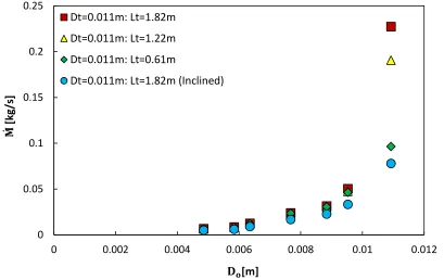
lengths and also for an inclined configuration. As suggested by the Beverloo correlation, it can

be seen that the tube length has no effect on the mass flow rate when in the choked regime. On

the other hand, the flow rates increased with increasing tube length in the dilute regime. For

the inclined tubes, though the overall trend agreed with the Beverloo correlation, however the

mass flow rates are less than with the vertical tubes. In this configuration, the effective gravity

along the tube would be less. In addition, there would be a skewed free-fall arch at the orifice

exit that could result in different values for 𝐶 and 𝑘. More study needs to be done to obtain a

clearer understanding of this phenomenon.

Figure 3.3 Flow behavior for different tube lengths and inclinations

0 0.05 0.1 0.15 0.2 0.25

0 0.002 0.004 0.006 0.008 0.01 0.012

Dt=0.011m: Lt=1.82m

Dt=0.011m: Lt=1.22m

Dt=0.011m: Lt=0.61m

Dt=0.011m: Lt=1.82m (Inclined)

̇

𝐌

[kg

/s

]

(30)

Chapter 4

Simulation Setup

The multiphase modelling of dry granular flows deals with the exchange of momentum

between the continuum and dispersed phases – air and particles. This was resolved by a

implementing a Lagrangian method. In dense flow regimes, due to the high packing fractions

of the dispersed phase (~60%), the inter-particulate interactions become frequent and

accounting for their behavior is necessary to resolve the flow state. Though the continuum can

be solved using the conventional Navier-Stokes equations, the collisional and contact

interactions of the particles among themselves and with other boundaries need to be modelled

for a precise simulation of the flow. This was achieved by considering the Discrete Element

Method (DEM) which computes contact forces for each and every particle. The following

sections gives a complete picture of how the simulation modelling was done in this research.

4.1 Discrete Element Method

The Lagrangian Multiphase model solves the equation of motion for representative parcels

of the dispersed phase as they pass through the solution domain. It is primarily suited for

(31)

particles, droplets, or bubbles[27]. Using this approach is the best way to resolve interactions

of the discrete phase with physical boundaries.

The Discrete Element Model, is an extension of the Lagrangian Multiphase approach. In

this approach the inter-particulate contact forces are explicitly accounted. This numerical

approach is typically suited for simulating motion of many interacting discrete objects that are

usually solid particles. Though DEM modelling requires significant computing power, it

provides a detailed resolution that other approaches cannot achieve. This model was primarily

established by Cundall and Strack [10], where the inter-particle contact forces are included in

the equation of motion.

The application of DEM can be broadly classified into two types – hard-particle and

soft-particle approaches. While the former is suitable for rapid granular flows, the latter which

allows multiple and enduring contacts between particles is appropriate for dense flows [28].

Thus the soft-particle approach was chosen in the current study. Here the term “soft-particle”

refers to the fact that the particles can deform during a contact. But calculating the structural

deformation of each and every particles in the simulation would be computationally intensive.

To avoid that, each particle is considered to remain geometrically rigid but are allowed to

overlap with contact boundaries. The amount of overlap is considered analogous to the

deformation at the contact boundary and the interaction forces are computed from the amount

of overlap using different contact models. Since the deformations of the individual particles

are relatively small in comparison with the deformation of the granular assembly (which is

primarily due to the movements of the particles as rigid bodies) as a whole, this assumption

(32)

representation of the mechanical behavior of the system. The contact duration is finite and the

multiple contacts may occur simultaneously in this approach. The soft-particle approach is a

more flexible method as compared to the hard-particle method because of the variety of force

models and particle shapes that can be accounted for. But on the other hand, it is typically a

more time consuming approach due to necessary small integration time steps

As a whole, DEM includes three steps – 1) contact and overlap detection, 2) force

calculation and 3) particulate motion. These individual computations are done continuously to

update the state of the particles (position and velocity vector of its center) and the flow. The

calculations performed in the discrete element method alternate between the application of

contact-force laws and the Newtonian displacement laws.

The solution state of each particle in the DEM methodology includes the particle centroid

location, particle radius, particle velocity and the forces acting on each particle. The

particle-particle overlap is calculated using the particle-particle centroid locations. The following sections

describe the governing equations involved in calculating the contact forces and the resulting

particulate motion.

4.1.1 Governing equations

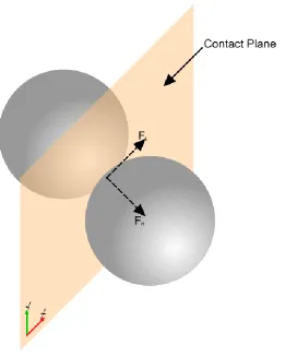
In the Discrete Element Method, the contact forces are usually divided into two

components – normal component and tangential component as shown in figure 4.1. The contact

force formulation is considered as a variant of the spring-dashpot model. The spring model is

used to generate the repulsive forces that act while the particles push against each other. On

the other hand, the dashpot model represents the viscous damping forces that come into action

(33)

of the particles in contact and the dashpot model signifies the inelasticity of the collisions

among them. To resolve the forces in both the directions – normal and tangential, the

particulate contacts are modeled as a pair of spring-dashpot oscillators with one for each

component.

Figure 4.1 Particle contact force formulation on the contact plane

In the current simulation studies, the Hertz-Mindilin no-slip contact model is used for

modelling the particle-particle and particle-wall contacts. This model is based on the

Hertz-Mindilin contact theory[29]. As described above, the contact force is divided into normal and

(34)

𝐹𝑐𝑜𝑛𝑡𝑎𝑐𝑡 = 𝐹𝑛𝑜𝑟𝑚𝑎𝑙+ 𝐹𝑡𝑎𝑛𝑔𝑒𝑛𝑡𝑖𝑎𝑙 (2)

Each force is calculated from the amount of overlap and the approach velocity at the point of

contact; the former for repulsive and the latter for damping. Based on this, the repulsive normal

contact forces are determined using the following equation:

𝐹𝑁 = −𝐾𝑁𝑂𝑁− 𝑁𝑁𝑉𝑁 (3)

where 𝐾_𝑁 is the normal spring stiffness, 𝑂_𝑁 is the normal overlap, 𝑁_𝑁 is the normal damping

coefficient and 𝑉_𝑁 is the normal approach velocity at the contact point. The subscript 𝑁 in all

these relations represent the normal direction. The normal spring stiffness is computed using

the following equation

𝐾_𝑁 =4

3𝐸𝑒𝑞√𝑂𝑁𝑅𝑒𝑞 (4)

where 𝐸𝑒𝑞 and 𝑅𝑒𝑞 are equivalent Young’s modulus and equivalent radius. They are computed

as follows:

𝐸𝑒𝑞 =

1 1 − 𝜈_𝐴2

𝐸𝐴 +

1 − 𝜈_𝐵2

𝐸𝐵

(5)

𝑅_𝑒𝑞 = ₁ 1 𝑅𝐴+

1 𝑅𝐵

(6)

Where 𝐸𝐴 and 𝐸𝐵 are Young’s moduli of the two particles in contact and 𝜈𝐴 and 𝜈𝐵 the

Poisson coefficients. The terms 𝑅_𝐴 and 𝑅_𝐵 are the radii of the two particles. On the other hand,

the normal damping coefficient is computed using the following equation:

𝑁𝑛 = √(5𝐾𝑁𝑚𝑒𝑞)𝑛𝑁𝑑𝑎𝑚𝑝 (7)

Where 𝑚_𝑒𝑞 and 𝑛_𝑁𝑑𝑎𝑚𝑝 are the equivalent mass and normal damping parameter. They are

(35)

𝑚_𝑒𝑞 = ₁ 1 𝑚𝐴+

1 𝑚𝐵

(8)

𝑛_𝑁𝑑𝑎𝑚𝑝 = − ln(𝐶𝑁

𝑟𝑒𝑠𝑡₎

√𝜋2_{+ ln(𝐶}

𝑁𝑟𝑒𝑠𝑡)2

(9)

where 𝑚_𝐴 and 𝑚_𝐵 are the masses of the two particles in contact. Here, 𝐶_𝑁𝑟𝑒𝑠𝑡 is the normal

coefficient of restitution between the two particles at the contact surface.

The contact forces in the tangential direction have similar relations only if the magnitudes

are less than the maximum possible value – the static friction value from the Coulomb friction

law. As a result, the tangential force representation takes the following form:

𝐹𝑇 = −𝐾𝑇𝑂𝑇− 𝑁𝑇𝑉𝑇 if |𝐾𝑇𝑂𝑇| < |𝐾𝑁𝑂𝑁|𝐶𝑓𝑠 (10)

𝐹𝑇 = (|𝐾𝑁𝑂𝑁|𝐶𝑓𝑠)_|𝑂𝑂𝑡

𝑡| if |𝐾𝑇𝑂𝑇| > |𝐾𝑁𝑂𝑁|𝐶𝑓𝑠 (11)

where 𝐾_𝑇 is the tangential spring stiffness, 𝑂_𝑇 is the tangential overlap, 𝑁_𝑇 is the tangential

damping coefficient and 𝑉_𝑇 is the tangential approach velocity at the contact point. Here, 𝐶_𝑓𝑠

represents the static friction coefficient between the contact surfaces. With subscript 𝑇

representing the tangential direction, all the properties are calculated in similar way as in

equations (4)-(9) except for the tangential spring constant which is a function of equivalent

shear modulus, 𝐺𝑒𝑞. It is calculated as:

𝐾_𝑡= 8𝐺_𝑒𝑞√𝑂𝑡𝑅𝑒𝑞 (12)

Here, the equivalent shear modulus is calculated as follows:

𝐺_𝑒𝑞 = 1

2(2 − 𝜈𝐴)(1 + 𝜈𝐴)

𝐸_𝐴 +2(2 − 𝜈𝐵 𝐸)(1 + 𝜈_𝐵 𝑩)

(36)

For particle-wall collisions, the formulas and the computations stay the same. But the wall

radius and masses are assumed to be 𝑅_{𝑤𝑎𝑙𝑙} = ∞ and 𝑀_{𝑤𝑎𝑙𝑙} = ∞. In this case, the equivalent

radius is reduced to 𝑅_𝑒𝑞 = 𝑅_{𝑝𝑎𝑟𝑡𝑖𝑐𝑙𝑒} and the equivalent mass would be 𝑀_{𝑤𝑎𝑙𝑙} = 𝑀_{𝑝𝑎𝑟𝑡𝑖𝑐𝑙𝑒}.

Once these forces are computed, the net force on a particle, resulting from both the normal

and tangential components of particle-particle and particle-boundary contacts is calculated in

the following manner:

𝐹𝐶𝑜𝑛𝑡𝑎𝑐𝑡 = ∑ 𝐹𝑐

𝑁𝑒𝑖𝑔ℎ𝑏𝑜𝑟𝑖𝑛𝑔 𝑃𝑎𝑟𝑡𝑖𝑐𝑙𝑒𝑠

+ ∑ 𝐹𝑐

𝑁𝑒𝑖𝑔ℎ𝑏𝑜𝑟𝑖𝑛𝑔 𝑏𝑜𝑢𝑛𝑑𝑎𝑟𝑖𝑒𝑠 (14)

These are used in the momentum balance equation of the material particles as follows:

𝑚_𝑝𝑑𝑣𝑝

𝑑𝑡 = 𝐹𝑆 + 𝐹𝐵+ 𝐹𝐶𝑜𝑛𝑡𝑎𝑐𝑡 (15)

where 𝐹𝐵 represents the body forces on the particles including gravity, while 𝐹𝑆 represents the

surface forces that include the pressure gradient force and drag force. Here 𝑚_𝑝 and 𝑣_𝑝 are the

mass and velocity of each material particle. Similarly, the DEM particle equations of motion

incorporate angular momentum conservation equations as:

𝑑

𝑑𝑡(𝐼𝑝𝜔𝑝) = ∑ 𝑇𝑐

𝑁𝑒𝑖𝑔ℎ𝑏𝑜𝑟𝑖𝑛𝑔 𝑃𝑎𝑟𝑡𝑖𝑐𝑙𝑒𝑠

+ ∑ 𝑇𝑐

𝑁𝑒𝑖𝑔ℎ𝑏𝑜𝑟𝑖𝑛𝑔 𝑏𝑜𝑢𝑛𝑑𝑎𝑟𝑖𝑒𝑠 (16)

where 𝐼𝑝 and 𝜔𝑝 are moment of inertial and angular velocity of the particle. The contact torque

is computed from the contact forces on the particles as:

𝑇_𝑐 = 𝑟_𝑐× 𝐹_{𝐶𝑜𝑛𝑡𝑎𝑐𝑡}− 𝜇_𝑟|𝑟𝑐||𝐹𝐶𝑜𝑛𝑡𝑎𝑐𝑡|

𝜔_𝑝

|𝜔_𝑝| (17)

where 𝑟_𝑐 is the vector from the particle’s center of gravity to the contact point and 𝐹_𝑐 is the

(37)

From these momentum balance equations, the linear and the angular velocity at the updated

time-steps are calculated. Using these values, the new position of the particulate network is

calculated and this cycle is repeated. Similar to the contact forces, the lift/drag forces can also

be modelled using different techniques available in the literature. But in the current dense

particle simulation study, it was observed that there was no influence of the interstitial air on

the particles. To validate this, two set of simulations were conducted, one by considering the

particle-continuum coupling and one without the coupling. In both the studies, the particulate

velocities, the particulate flowrates and all the other parameters of the granular flows remained

the same. In addition, the computational time and intensity of the problem was drastically

reduced when the coupling was removed. Hence, all the simulations studies in the current

research were conducted by ignoring the lift/drag/torque forces on the particles from the

continuum and the particle motion was only governed by the gravitational force and collision

interactions with other particles and rigid boundaries.

4.1.2 Numerical method

The governing equations of the particles were solved numerically in the Cartesian

coordinate system. Since the interstitial air and the particles were completely de-coupled, the

momentum equation of the continuum was not solved in the current studies. As a result, a

coarser mesh was used as the grid resolution had no direct influence on the flow. The general

purpose CFD code STAR-CCM+ [27] was used as the numerical solver to explicitly integrate

the governing equation. Its robust application of the aforementioned discrete element equations

made it the primary choice for the simulation studies. Attempts were made to solve the problem

(38)

in each simulation are huge, the data transfer and communication among each processor for

the computations increased and slowed down the solution even with the slightest increase of

processors. Hence, all the studies were conducted on a single core using Intel® Xeon®

E5-2687W processor.

A first order temporal discretization was used for the advancement of the solution state. A

major assumption in DEM simulations is that the effect of contact between two particles is

localized and does not propagate to the neighboring particles within a time-step[10]. Thus, the

time step size needs to be restricted for these computations. This was done by limiting it to the

time it takes the Rayleigh wave to propagate across the surface of the sphere to the opposite

pole [29][30]. This time is calculated as:

𝜏1 = 𝜋

𝑅_𝑚𝑖𝑛

𝑉𝑅𝑎𝑦𝑙𝑒𝑖𝑔ℎ (18)

where 𝑅𝑚𝑖𝑛 is the minimal particle radius. The Rayleigh wave velocity depends on the material

properties of the particle. In addition, the time-step size is also limited by the duration of impact

of two perfectly elastic spheres. This time is calculated as[31]:

𝜏₂ = 2.94 (5√2𝜋𝜌 4

1 − 𝜐2

𝐸 )

2

5 _𝑅

√𝑣𝑖𝑚𝑝𝑎𝑐𝑡

5 (19)

Finally, the third restriction on the time step size is based on the assumption that particles

must not move too far within the time-step. This prevents missing contacts between DEM

particles as well as particles and the wall. Thus, each particle is constrained such that it takes

at least 10 time-steps for the particle to move the full-length of the radius. Thus the restriction

(39)

𝜏₃ = 𝑅

𝑣_{𝑝𝑎𝑟𝑡𝑖𝑐𝑙𝑒} (20)

4.2 Simulation Methodology

The current sections explains the geometries modelled for these simulation studies and also

summarizes the different properties and parameters used. Similar to the experiments, the

simulations were also conducted in a batch-wise fashion. As a result, the geometry was

modelled exactly like the experimental setup with a batch funnel on the top of the tube and an

orifice at the exit.

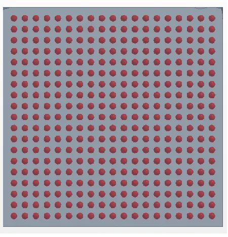
Figure 4.2 Particle injection into the solution domain using lattice structures

Before any flow was initiated, the entire solution domain was filled with particles by

keeping the exit orifice closed. The particles were added at every time step into the solution

domain and they settle down in the tube and the funnel due to the gravitational force acting on

(40)

particles at every lattice point, if a free space was available. In this way, the amount of

computational effort in setting up the simulation (adding particles alone) was avoided. Figure

4.2 gives a clear representation of the process. Once the entire solution domain is filled

completely, the flow is initiated by removing the orifice block. Finally, the required solution

scalars and vectors are recorded at every time step and further post-processing was done to

obtain necessary and meaningful results.

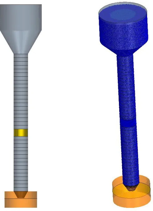
4.2.1 Geometry

As mentioned earlier the simulation geometry includes a funnel at the top and an orifice at

the bottom end of the tube. All the simulation studies were conducted with only a vertical

configuration. Initially, the simulation geometry was set with a tube as long as the one used in

the experiments. But as a result, the number of particles in the solution domain was huge

slowing down the computational process. As discussed in the previous sections, the length of

the tube, once longer than the saturation length (explained later), had no influence on the dense

flow regime. Similar flow rates were obtained in all the cases with different tube lengths.

Though the internal flow profile might be vary with tube length, to reduce the computational

cost, the simulations were done with shorter tube lengths. Figure 4.3 shows the geometry used

in the simulations.

In the current research, each of the simulation cases with a specific tube diameter, tube

length, and particle diameter was performed with different orifice openings. This was done to

observe the flow physics for different flow rates (as understood from the Beverloo studies

performed in the preliminary experiments). It was mentioned earlier that every simulation takes

(41)

particles. Hence, it would not be wise to repeat the same for each and every orifice diameter.

To avoid that, the simulation geometry was modelled in such a manner that the filling was

performed only once and the orifice opening can be changed after being filled.

Figure 4.3 Simulation geometry without and with particles (left to right)

4.2.2 Properties and parameters

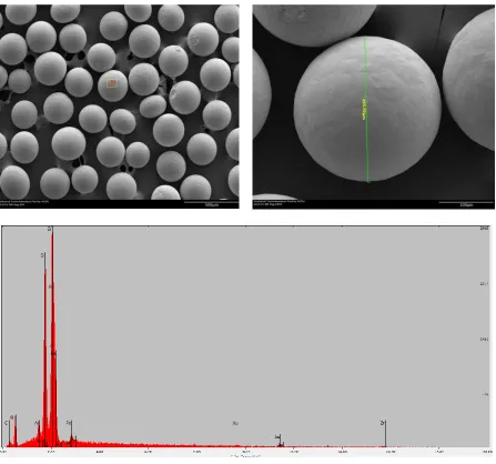
To observe the particle surface more clearly, Scanning Electron Microscopic images were

(42)

microscope to get the images. It also enabled in identifying the composition of the sample

using X-Ray energy spectrum.

Figure 4.4 (clockwise) (i) SEM image of particulate sample at 10X magnification (ii) SEM

image of particulate sample at 50X magnification (iii) Energy spectrum of the particulate

(43)

It was identified that the particle diameter ranges from 275 microns to 330microns. The

particles were found to be mostly spherical and have a smooth outer surface. From the spectral

imaging at point S1 in, the particle chemical composition was found with Silica and Zirconia

as the dominant constituents. Similar to these experimental samples, a distribution of

particulate sizes can be used for the simulation studies. But this would make the computational

process intensive as every particle should have its own radius instead of having a constant

value for the entire batch. As a result, mono-sized spherical particles were used in all the

simulation studies.

The different properties required for the simulation studies include, particle density,

particle Young’s modulus, particle Poisson’s ratio, particle-particle/particle-wall static/rolling

friction and particle-particle/particle-wall coefficient of restitution. The density of the particles

is experimentally calculated by adding a known mass of particles in a beaker of water. Since

the porosity of the particle is low, as they are added into water, the water level rises. The change

in the volume of the water would be equal to the volume of the particles. In this way the volume

of the known mass of particles is found and eventually the density was calculated using the

relation 𝜌 =_{𝑣𝑜𝑙𝑢𝑚𝑒}𝑚𝑎𝑠𝑠 . The Young’s modulus and the Poisson’s ratio of the particles (Si-Zr) are

obtained from the Catalogue provided by the suppliers. For both particle and

particle-wall, two coefficients of restitution are required in the simulations – one in the normal direction

and one in the tangential direction. They signify the amount of kinetic energy (momentum)

lost in the event of a collision. In the current scope of studies, the packing fractions inside the

flow domain are close to 60%. As a result, the number of continuous contacts among particles

(44)

events leading to a weak or no influence of restitution on the flow[16]. This assertion was also

verified from the simulations by running cases with different restitution coefficient while

keeping all the other parameters constant. This was performed for all four values of restitution

coefficients. It was observed that the mass flow rates inside the tube remained constant in all

the cases, even though the restitution coefficient was varied. As a result, best guess values and

data available from the material catalogues were considered for the coefficients of restitution.

To identify the particle-particle friction, the angle of repose was used. It is the steepest

angle of descent or dip relative to the horizontal plane to which the material can be piled

without slumping[32]. At this angle, the material on the slope face is on the verge of sliding.

When bulk granular materials are poured onto a horizontal surface, a conical pile will form. It

is the internal angle between the surface of the pile and the horizontal surface that is defined

as the angle of repose. It is primarily dependent to the density of the particles, the surface area

and the coefficient of friction of the material (particle-particle friction).Using this idea,

simulations were conducted with different particle-particle friction values and the

corresponding angle of repose was calculated in each case. This was done by initially adding

particles in a conical structure such that they are completely at rest. Once the particles are

settled, the conical wall around them was removed and the particles slowly settle at their

normal angle of repose. In this way, for different particle-particle frictions, the angle of repose

was computed. The process is clearly illustrated in figure 4.5. It was experimentally identified

that for the granular material used in the experimental studies had an angle of repose of 26o.

Thus, the particle-particle friction for which the same angle of repose was computationally

(45)

Figure 4.5 Methodology used to calculate the angle of repose using simulations

The particle-wall friction on the other hand is difficult to measure experimentally. Hence

it was identified indirectly from the simulations. From the previous experimental studies, the

flowrates for different orifice diameters were identified. Similar orifice geometry was

modelled for the simulation and the particle-wall friction was tuned such that the flow rate

matches those from experiments. This friction values was also verified with orifice diameters

and the experimental flow rates. Hence, the particle-wall friction was found to have identified.

Rolling friction is another property that needs to be assigned for the simulations. Similar to the

restitution coefficients, the rolling friction also had absolutely no influence on the overall flow Angle of

(46)

rates. This might again be due to the high packing fraction in the flow domain. As a result a

best guess value was assigned to these parameters. The following table describes all the

properties used for the simulation studies.

Table 4.1 Particulate properties for the simulation studies

Diameter 0.0003 m

Density 3934.06 kg/m3

Young’s Modulus 75800 MPa

Poisson’s Coefficient 0.235

Static Friction Coefficient Particle-Particle _{Particle-Wall} 0.8 _0.5

Rolling Friction Coefficient Particle-Particle _{Particle-Wall} 0.001 _0.001

Normal Restitution Coefficient Particle-Particle _{Particle-Wall} 0.6 _0.5

Tangential Restitution Coefficient

Particle-Particle 0.8

Particle-Wall 0.5

4.2.3 Run cases

The entire simulation study was divided into two broad groups – Short tube measurements

and Long tube measurements. The short tube measurements are primarily used to understand

the radial profiles of velocities, packing fractions and flow parameters like flow rates and

particle-wall contact behavior, while the long tube measurements are used to understand the

axial profiles of these quantities and observe the temporal internal flow characteristics along

the tube axis.

For the short-tube simulations, three tube diameters of 5mm, 7.747mm and 10.922mm

were studied. The tube lengths in these cases were 0.05m, 0.075m and 0.1m respectively.

(47)

the wall-pressure saturates (explained in detail in next sections). All these cases were computed

with 10-15 different orifice sizes to observe the variation of flow rheology at different mass

fluxes through the tube. The main parameters that are recorded in these simulations are;

particulate velocities, particle-wall contact forces, particulate flow rate through the orifice,

particle-wall contact points, and packing fraction profiles. To understand the influence of

particle diameter on the flow physics, simulations were done in a 7.747m diameter tube with a

length of 0.075m. Particles of 300µm, 475µm and 600µm were studied in these simulations.

Each case is again computed for different orifice sizes (flow rates). The short-tube simulations

involved in solving around 500,000 particles in the computational domain.

The main motivation for the conducting long-tube measurements is to study the flow

fluctuations. In short-tube measurements, it was observed that the flow fluctuations amplify at

higher axial locations above the orifice (explained in detail in next sections). To observe and

quantify this behavior, the simulations were conducted with a tube of 0.3m in length. The tube

diameter in these studies was 7.747 mm and particles of 300µm in diameter were used. These

studies were conducted on 4 different orifice sizes to understand the influence of mass flux on

these fluctuations. In addition, the axial profiles of aforementioned quantities, profiles of mass

flow rates at different axial locations inside the tube were also obtained through these studies.

Since the long-tube simulations involved solving around a million particles in the solution

domain, they took relatively longer computational time than the short-tube simulation. The

subsequent sections present the various results and observations made in the simulations

(48)

Chapter 5

Simulation Results and Discussions

The simulation studies, which were conducted in batches were validated by comparing

them with the experimental data. Since the flow rates are the only measurements in the

experiments, they were used for this verification. Hence tube-orifice geometries were matched

to the exact dimensions as in the experiments. The flow rates were measured by calculating

the number of particles crossing the orifice exit per unit time. This tracking was done over a

period of time and a thus temporal evolution of the flow rates was found.

Similar to the experiments, the flow rates remained constant throughout the granular

batch. In figure 5.1, the flow rates obtained for different orifice sizes were plotted for both the

experiments and the simulations. This was done for both the tubes of diameter 7.747m and

10.922m. It can be observed that the data matched perfectly and have similar trends. The

Beverloo trend is also followed by the simulation results. Similar to the experiments, the

simulation mass flow rates also deviated from the Beverloo Law after a critical mass flow rate

was exceeded. All these observations will be further explained in the future sections, but for

now, this validation study suggests that the simulation methodology and parameters give good

(49)

Figure 5.1 Validation of flow rates obtained in the Discrete Element simulations

The following sections briefly describe the important observations made for dense granular

flows in cylindrical tubes. Though the simulations were performed on a Cartesian coordinate

system, a cylindrical system was used to discuss the results with z as the axial, r as the radial

and θ as the angular directions, respectively.

5.1 Particulate velocity profiles

As mentioned earlier, the solution state for each particle includes the position and velocity.

To obtain the velocity profiles, the velocity of particles were recorded and the required

data-processing was done. But since each simulation involves a large number of particles, it would

be computationally intensive to track/record the state of every particle. As a result, the velocity

profiles were obtained indirectly using the method of Boundary Sampling[27] (discussed

further in this section). 0

0.03 0.06 0.09 0.12 0.15

0 0.002 0.004 0.006 0.008 0.01 0.012

Expt: Dt=0.008m Expt: Dt=0.011m Sim: Dt=0.008m Sim: Dt=0.011m Beverloo Correlation

̇

𝐌

[kg

/s

]

(50)

Figure 5.2 Contour plots of particulate velocities (a) through the orifice (b) through a flow

cross-section

The particulate velocities were observed over time using contour plots. They are plotted

for a specific case at an intermediate time-step in figure 5.2. Based on the color legend and the

(51)

It can also be observed that the particles near the walls have a lower velocity as compared to

the ones at the core. It is important to observe that the flow remains uniform at all polar angles

in the cross-section. As the particles exit the tube, due to the orifice they accelerate. This can

be seen in the contour plot from the red shade at the orifice exit. Finally it can be seen that the

particles have a slip velocity at the walls similar to all granular flow configurations.

Though the contour plots give a rough overview of the velocities and the animations made

from them depict the flow fluctuations, the time averaged velocities and the radial profiles are

necessary to gain a clear understanding of the flow. As mentioned earlier, the boundary

sampling method is used to obtain velocity profile information. In this technique, the data

recording occurs only at certain instances in the simulation. The recording event can be

triggered by setting different criterion on the particles. In the present case, the data recording

event was set to trigger whenever a particle crosses a specific plane or a specific sampling

region. For example, if there are 1000 particles in a cylindrical solution domain, but only 50

particles in contact with the bottom face of the cylinder, the solution state of the 50 particles

alone can be accessed by using the bottom face as the sampling boundary. Similarly, as another

example, if the particles are crossing a plane in a solution domain, the data recording event can

be specifically triggered for particles that are on or just crossed the plane at a specific time

step. In this way, the data recording will occur throughout the solution time at every time-step

but only for those particles that are on or just crossed the plane of concern (sampling boundary).

The boundary sampling method thus stands as a robust and efficient way of accessing the data

(52)

In the current scenario, to obtain the radial profiles of velocity, the flow cross-section is

divided into annular rings of different radii as shown in figure 5.3. Every annular ring is a

single plane that is located at a specific radial location. Using boundary sampling, the velocity

data is recorded for all the particles that come in contact or just cross a specific annular plane.

This is analogous to measuring the velocity of all the particles that are at that specific radial

location. Finally taking the average of the velocity data for that annular plane gives the

particulate velocity at that specific radial location at that time-step. This is primarily based on

the observation that the particles have similar flow behavior at different polar angles, i.e.

axisymmetric flow. In this way, the same process is repeated on all the annular sections and is

continued at every time step. Thus, the temporal evolution of particulate velocities at different

radial locations is obtained using the method of boundary sampling. Since a boundary layer

was expected near the tube walls, to capture it precisely, the annular sections were not made

of uniform thickness but are thinner near the wall. This is analogous to using a prism mesh to

resolve the boundary layer in continuum flow problems.

(53)

It was observed that the magnitudes of the radial and angular velocities were negligible as

compared to the axial velocities. As a result, from this point on, the term “velocity” refers to

the axial velocity of the flow. From the time evolution of velocity at different radial locations,

it was observed that the velocities fluctuate about a mean value. This can be observed in figure

5.4 which was plotted for an orifice with tube diameter of 7.747mm and particles of 300 micron

in diameter. The different colors in the plots represent a different radial location at a specific

axial location. Though fluctuations make it look erratic, every radial location had a mean

velocity. The velocity fluctuations describe the intermittent and rearranging nature of the

particulate flows. Though not plotted in the current discussion, it was observed that the velocity

fluctuations were higher at the tube wall as compared at the core of the tube. This signifies that

the particles are undergoing relatively higher re-arrangement in the wall region.

Figure 5.4 Time evolution of particulate velocities at different radial locations

-0.08 -0.07 -0.06 -0.05 -0.04 -0.03 -0.02 -0.01 0

0.5 1 1.5 2 2.5 3

(54)

To understand the internal flow profile more thoroughly, time averaged velocity plots were

obtained from the temporal data. It important to understand that the velocity data is obtained

only when a particle crosses through or stays on the annular plane. For slower flow rates, there

would be a scenario where no particle crosses the sampled boundary and as a result no data

would be recorded at those time steps. This is a direct result of the discrete nature of the

granular flow. As a result, the time-averaging for this data set should be ensemble averaging.

Since we are dealing with vertical tubes and the flow is a gravity-driven configuration, the

axial components of the particulate velocities would be of negative magnitudes as the gravity

acts in negative z-direction of the flow. In figure 5.5, the time averaged velocity was plotted

versus the radius of the cross-section for a flow rate of 3.5g/s.

Figure 5.5 Time averaged particulate velocity at 3.5g/s mass flow rate (tube diameter:

0.007747m and particle diameter: 300 microns) -0.04

-0.035 -0.03 -0.025 -0.02 -0.015 -0.01 -0.005 0

-0.004 -0.003 -0.002 -0.001 0 0.001 0.002 0.003 0.004

V

e

lo

ci

ty

[m

/s

]

Radial Location [m]

Velocity

Experimental and Computational Studies of Gravity-Driven Dense Granular Flows.

DEDICATION

BIOGRAPHY

ACKNOWLEDGMENTS

TABLE OF CONTENTS

LIST OF TABLES

LIST OF FIGURES

Chapter 1

Introduction

Chapter 2

Experimental Setup

2.1 Design

2.2 Methodology

2.3 Run cases

Chapter 3

Experimental Results

3.1 Variation of flow rates with orifice diameters

3.2 Influence of tube length, diameter and inclination on the flow

Chapter 4

Simulation Setup

4.1 Discrete Element Method

4.1.1 Governing equations

4.1.2 Numerical method

4.2 Simulation Methodology

4.2.1 Geometry

4.2.2 Properties and parameters

4.2.3 Run cases

Chapter 5

Simulation Results and Discussions

5.1 Particulate velocity profiles