A Study of Densities and Viscosities of Multi-Component Regular LiquidSystems at 293.15K and 298.15K

(1)

Electronic Theses and Dissertations Theses, Dissertations, and Major Papers

2013

A Study of Densities and Viscosities of Multi-Component Regular

LiquidSystems at 293.15K and 298.15K

Niloufar Mohajerani University of Windsor

Follow this and additional works at: https://scholar.uwindsor.ca/etd Part of the Civil and Environmental Engineering Commons

Recommended Citation Recommended Citation

Mohajerani, Niloufar, "A Study of Densities and Viscosities of Multi-Component Regular LiquidSystems at 293.15K and 298.15K" (2013). Electronic Theses and Dissertations. 4916.

https://scholar.uwindsor.ca/etd/4916

This online database contains the full-text of PhD dissertations and Masters’ theses of University of Windsor students from 1954 forward. These documents are made available for personal study and research purposes only, in accordance with the Canadian Copyright Act and the Creative Commons license—CC BY-NC-ND (Attribution, Non-Commercial, No Derivative Works). Under this license, works must always be attributed to the copyright holder (original author), cannot be used for any commercial purposes, and may not be altered. Any other use would require the permission of the copyright holder. Students may inquire about withdrawing their dissertation and/or thesis from this database. For additional inquiries, please contact the repository administrator via email

(2)

Regular Liquid Systems at 293.15 K and 298.15 K

By

Niloufar Mohajerani

A Thesis

Submitted to the Faculty of Graduate Studies Through Environmental Engineering In Partial Fulfillment of the Requirements for The Degree of Master of Applied Science at the

University of Windsor

Windsor, Ontario, Canada 2013

(3)

by

Niloufar Mohajerani

APPROVED By:

Dr. Nader G. Zamani

Department of Mechanical, Automotive and Materials Engineering

Dr. Shaohong Cheng

Department of Civil and Environmental Engineering

Dr. Abdul-Fattah A. Asfour, Advisor

Department of Civil and Environmental Engineering

(4)

I hereby certify that I am the sole author of this thesis and that no part of this thesis has been published or submitted for publication.

I certify that, to the best of my knowledge, my thesis does not infringe upon anyone’s copyright nor violate any proprietary rights and that any ideas, techniques, quotations, or any other material from the work of other people included in my thesis, published or otherwise, are fully acknowledged in accordance with the standard referencing practices. Furthermore, to the extent that I have included copyrighted material that surpasses the bounds of fair deling within the menaing of the Canada Copyright Act, I certify that I have obtained a written permission from the copyright owner(s) to include such material(s) in my thesis and have included copies of such copyright clearances to my appendix.

I declare that this is a true copy of my thesis, including any final revisions, as approved by my thesis committee and the Graduate Studies office, and that this thesis has not been submitted for a higher degree to any other University of Institution.

(5)

iv

propanol + 1-octanol and its quaternary, ternary and binary subsystems were measured and reported at

293.15 K and 298.15 K.

The experimental data obtained during the course of the present study were employed to test the

predictive capabilities of six selected viscosity models available in the literature; viz., the generalized

McAllister model, the pseudo-binary McAllister model, the group contribution GC-UNIMOD model, the

generalized corresponding state principle model (GCSP), the Allan and Teja correlation, and the

Grunberg and Nissan law of viscosity.

The results of testing indicated that the pseudo-binary McAllister model predicted the experimental data

better than the other models. Such a result is not in agreement with previous studies due to the relatively

high size ratio of molecules of the components constituting some systems as well as differing shapes of

(6)

v

This thesis is dedicated to my parents ‘Nasrin Saatchi’ and ‘Mansour Mohajerani’, for their

(7)

I would like to express my sincere appreciation to my Professor Dr. Abdul-Fattah A. Asfour for

giving me this opportunity and guiding me through all steps with his knowledge and kindness.

I would like also to thank my parents who supported me from overseas these years both

financially and emotionally through all problems I faced in the new chapter of my life. I am also

thankful to my brother, Masroor, who gave me confidence and the power to overcome my pains

and keep following my dreams.

My thanks also go to professors in the Environmental Engineering program at the University of

Windsor who mentored me with their knowledge and experience.

I would also express my deep appreciation to my special friends, Ali, Aida, Hanif and Bart for

being examples of true friends and who helped me to deal with pains.

(8)

vii

AUTHOR’S DECLARATION OF ORIGINALITY……….………..………..iii

ABSTRACT………...………iv

DEDICATION………..………...v

ACKNOWLEDGEMENTS.………...………vi

LIST OF TABLES………...x

LIST OF FIGURES………..xiv

CHAPTER 1 INTRODUCTION……….1

1.1 General…..……….1

1.2 Objectives ………..3

1.3 Contributions and Significance………..5

CHAPTER 2 PERTINENT LITERATURE REVIEW………...6

2.1 General………...6

2.2 The Semi-Theoretical Models for Predicting the Viscosity of Liquid Mixtures……...7

2.2.1 The McAllister three-body interaction model……….7

2.2.1.1. Three-body interaction model for a binary mixture liquid system………...11

2.2.1.2. Extension of the McAllister three-body model to ternary liquid systems …….………...16

2.2.1.3. Conversion of the McAllister model from a correlative to a predictive model……….17

2.2.1.4. The generalized McAllister three-body model ………22

2.2.2 The pseudo-binary McAllister model………...27

2.2.3 The group contribution (GC-UNIMOD)………..28

(9)

viii

2.3.2 The Grunberg and Nissan mixture law for viscosity...35

CHAPTER 3 EXPERIMENTAL PROCEDURES AND EQUIPMENT………..38

3.1 General..………...38

3.2 Materials……….……….38

3.3 Preparation of Solutions………..……….40

3.4 Density Measurements………..………...40

3.5 Viscosity Measurements…………..………43

CHAPTER 4 EXPERIMENTAL RESULTS AND DISCUSSION………...…………...47

4.1 General………..………...47

4.2 Calibration of the Density Meter………..………...47

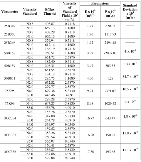
4.3 Calibration of Viscometers………..48

4.4 Composing the Liquid Solutions……….52

4.5 Testing the Predictive Capability of the Viscosity Models………...107

4.5.1 Testing the generalized McAllister three-body interaction model……….108

4.5.2 Testing the predictive capability of the pseudo-binary McAllister model………..117

4.5.3 Testing the predictive capability of the GC-UNIMOD model…………...124

4.5.4 Testing the predictive capability of the Grunberg and Nissan mixture law of viscosity ………..131

4.5.5 Testing the predictive capability of the Allan and Teja correlation………138

(10)

ix

tested……….153

CHAPTER 5 CONCLUSION AND RECOMMENDATIONS………..160

5.1 Conclusions………160

5.2 Recommendations….………..………...164

NOMENCLATURE……….………...165

REFERENCES……….……….…..168

APPENDICIES………..………..174

(11)

x

3.1 Gas Chromatography Analysis Results of the Pure Components 39

4.1 Calibration Data for the Density Meter at 293.15 K 49

4.2 Calibration Data for the Density Meter at 298.15 K 49

4.3 Calibration Data for the Viscometers at 293.15 K 50

4.4 Calibration Data for the Viscometers at 298.15 K 51

4.5 Densities and Viscosities of the Pure Components and their Corresponding

Literature Values at 293.15 K.

53

4.6 Densities and Viscosities of the Pure Components and their Corresponding

Literature Values at 298.15 K.

54

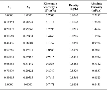
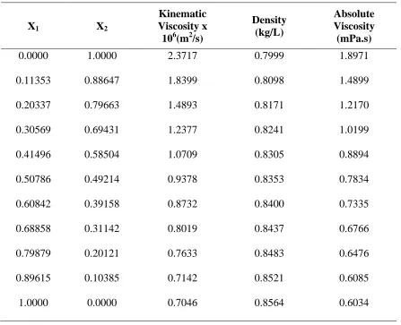
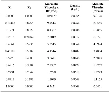
4.7 Densities and Viscosities of the Binary System: Cyclohexane (1)+p -Xylene (2) at 293.15 K.

55

4.8 Densities and Viscosities of the ternary system: Cyclohexane (1) + p-Xylene (2) + Chlorobenzene (3) at 293.15 K.

75

4.9 Densities and Viscosities of the quaternary system: Cyclohexane (1) + p

-Xylene (2) + Chlorobenzene (3) + 1-Propanol (4) at 293.15 K.

95

4.10 Densities and Viscosities of the quinary system: Cyclohexane (1) + p-Xylene (2) + Chlorobenzene (3) + 1-Propanol (4) + 1-Octanol (5) at 293.15 K.

105

4.11 The Effective Carbon Numbers of the Pure Compounds used in the Present

Study.

110

4.12 Test Results for the Generalized Mc Allister Three-Body Interaction Model

Employing the Experimental Kinematic Viscosity and Density Data of the

Binary Systems .

111

Ternary Systems.

113

(12)

xi Quaternary Systems.

Quinary Systems.

116

4.16 Test Results for the pseudo-binary Mc Allister Three-Body Interaction Model

Binary Systems.

118

Ternary Systems.

120

Quaternary Systems.

122

Quinary Systems.

123

4.20 Test Results for the GC-UNIMOD Model Employing the Experimental

Kinematic Viscosity and Density Data of the Binary Systems.

125

Kinematic Viscosity and Density Data of the Ternary Systems.

127

Kinematic Viscosity and Density Data of the Quaternary Systems.

129

Kinematic Viscosity and Density Data of the Quinary Systems.

(13)

xii

4.25 Test Results for Grunberg and Nissan Model Employing the Experimental

134

136

137

4.28 Test Results for the Allan and Teja Model Employing the Experimental

Kinematic Viscosity and Density Data of the Binary Systems.

139

141

143

144

4.32 Test Results for the GCSP Model Employing the Experimental Kinematic

Viscosity and Density Data of the Binary Systems.

146

Viscosity and Density Data of the Ternary Systems.

148

Viscosity and Density Data of the Quaternary Systems.

150

Viscosity and Density Data of the Quinary System.

151

(14)

xiii

(15)

xiv

2.2 Types of interactions in a Binary System, Three –Body Interaction Model 12

2.3 Types of Interactions in a Binary Mixture, Four –Body Interaction Model 13

2.4 Variation of the lumped parameter ν12/(ν1ν1ν2)1/3 with 1/T systems for which |N2-N1|≤3

19

2.5 Variation of the Lumped Parameter ν12(ν1 2_ν

1)-1/3 versus [(N2-N1)2/(N1 2

N2)1/3] 20

2.6 Kinematic Viscosity for n-alkanes versus the Effective Carbon Number (ECN) 23

3.1 The Anton-Paar Density Meter Unit and The temperature Control Chamber 42

3.2 The Cannon – Ubbelohde Glass Capillary Viscometer 45

3.3 The CT–1000 Viscosity Bath and the Omega Precision Thermometer 46

4.1 Graphical Representation of the Predictive Capabilities of the Viscosity

Models Using Binary System Data.

156

Models Using Ternary System Data.

157

Models Using Quaternary System Data.

158

(16)

CHAPTER 1

INTRODUCTION

1.1 GENERAL

Viscosity is the transport property of a fluid which characterizes resistance to flow. Viscosity

represents the concept of internal friction between the molecules of the fluid when any part of a

fluid moves; adjacent layers tend to be carried along too. In engineering processes such as heat

and mass transfer, the information about viscosity of liquid mixtures is important because viscosity

data show the behavior of liquid mixtures. Viscosity is the quantity that determines the forces to be

overcome when fluids are pumped through pipelines and in bearings, etc.

The shear stress F is defined as the shearing force, P, divided by the area A over which it acts. The

velocity gradient D equals the velocity difference v divided by the distance between the surfaces h.

In Newtonian liquids, the shear stress is directly proportional to the velocity gradient:

F = - µ D (1.1)

Equation (1.1) is known as Newton’s law of viscosity. The constant µ is the absolute viscosity which

has the units, g. cm-1.s-1, and is known as the ‘poise’ in honor of Poiseuille, one of the great pioneers

of viscometry. In glass viscometers, the liquid flows through a capillary due to gravity that means the

head of the liquid is the driving pressure. These types of viscometers measure the kinematic viscosity

ν of the fluid since the measurement is proportional to the density of the liquid.

(17)

Viscosity is a function of temperature. In gases, the viscosity increases with increasing the

temperature whereas in liquid systems, viscosity decreases with increasing temperature often by an

appreciable amount. Therefore, temperature control is exercised during all viscosity

measurements, and viscosity values should be tabulated with temperature. Also, in liquid mixtures

viscosity depends on composition as well as temperature.

The mechanisms and molecular theory of gas viscosity have been reasonably well clarified by

non-equilibrium statistical mechanics and the kinetic theory of gases (Millet, et al. 1996) but the

theory of liquid viscosity is less well developed. This lack of knowledge is because of the

uncertainty about the structure of liquids and the intermolecular forces among molecules in the

liquid state. It is particularly desirable to determine liquid viscosities from experimental data when

such data exist. In an attempt to solve this problem researchers are working to develop theories for

calculating the viscosities of liquid mixtures.

The problem associated with the structure of liquids was recognized and indicated by Asfour

(1980). He suggested classifying liquid solutions into three classes, viz., n-alkane mixtures, regular

solutions, and associated systems. That classification led to the successful prediction of the

dependence of mutual diffusivities on composition for different liquid systems (Asfour, 1985,

Dullien and Asfour, 1985, and Asfour and Dullien, 1986). Asfour and co-workers successfully

extended this classification to the prediction of the viscosities of multi-component liquid systems

for n-alkane liquid systems and regular solutions.

The methods of calculating the viscosity of liquids in the literature is classified into two categories,

(18)

latter require pure component and molecular parameters. Many of the existing methods are not

predictive and require viscosity data to determine adjustable parameters or, for mixtures interaction

parameters.

In the present study, the empirical and semi-theoretical models are presented and their predictive

capabilities are tested. Semi-theoretical models refer to those models which have a theoretical

basis but contain adjustable parameters which can be determined from experimental data. Such

models include: The generalized McAllister three-body interaction model, the pseudo-binary

McAllister interaction model, the GC-UNIMOD model, the generalized corresponding state

principle (GCSP) model, the Allan and Teja model, and the Grunberg and Nissan model

1.2 Objectives

Experimental data on multi-component liquid systems are scarce in literature. Ternary and

quaternary systems data are rare in the literature whereas for quinary liquid systems, Dr. Asfour’s

laboratory is the only laboratory in the world to report such data.

The main objectives of the present study are as follows:

- Measuring the kinematic viscosities and densities of the quinary regular system:

cyclohexane + p-xylene + chlorobenzene + 1-propanol + 1-octanol and its binary, ternary

and quaternary subsystems over the entire composition range at 293.15 K and 298.15 K.

- Testing the predictive capabilities of the selected viscosity models using the experimental

data obtained in the present study.

(19)

Table 1.1: The Systems Investigated in the Present Study

1. The binary subsystems of the quinary system: cyclohexane + p-xylene + chlorobenzene + 1-propanol + 1-octanol

cyclohexane (1) + p-xylene (2) cyclohexane (1) + chlorobenzene (2) cyclohexane (1) + 1-propanol (2) cyclohexane (1) + 1-octanol (2) p-xylene (1) + chlorobenzene (2) p-xylene (1) + 1-propanol (2) p-xylene (1) + 1-octanol (2)

chlorobenzene (1) + 1-propanol (2) chlorobenzene (1) + 1-octanol (2) 1-propanol (1) + 1-octanol (2)

2. The ternary subsystem of the quinary system : cyclohexane + p-xylene + chlorobenzene + 1-propanol + 1-octanol

cyclohexane (1) + p-xylene (2) + chlorobenzene (3) cyclohexane (1) + p-xylene (2) + 1-propanol (3) cyclohexane (1) + p-xylene (2) + 1-octanol (3)

(20)

Table 1.1 Cont’d.

3. The quaternary subsystem of the quinary system : cyclohexane + p-xylene +

chlorobenzene + 1-propanol + 1-octanol

cyclohexane (1) + p-xylene (2) + chlorobenzene (3) + 1-propanol (4) cyclohexane (1) + p-xylene (2) + chlorobenzene (3) + octanol (4) cyclohexane (1) + p-xylene (2) + 1-propanol (3) + 1-octanol (4) cyclohexane (1) + chlorobenzene (2) + 1-propanol (3) + 1-octanol (4) p-xylene (1) + chlorobenzene (2) + 1-propanol (3) + 1-octanol (4)

4. The quinary system : cyclohexane (1) + p-xylene (2) + chlorobenzene (3) + 1-propanol

(4) + 1-octanol (5)

1.3 Contributions and Significance

The density, kinematic viscosity and absolute viscosity values reported in the present study

provide reliable and valuable additions to the literature for the quinary system: cyclohexane +

p-xylene + chlorobenzene + 1-propanol + 1-octanol, and its binary, ternary and quaternary

sub-systems over the entire composition range at 293.15 K and 298.15 K.

(21)

CHAPTER 2

PERTINENT LITERATURE REVIEW

2.1 General

In engineering problems, calculation of viscosity of liquid mixtures plays an important role.

Knowledge of viscosity dependence on composition in different aspects of engineering is

important in the areas of heat, mass transfer, and fluid mechanics. Accordingly, authentic methods

for calculating the viscosity of liquid mixtures are required in industry.

In the literature, methods are available for viscosity prediction which are presented in this chapter.

These methods can be categorized into two types of models, viz., semi-theoretical and empirical.

The semi-theoretical models depend on theory and experimental data whereas the empirical

models are dependent on the acquisition of costly and time consuming experimental data.

In recent years, there have been efforts to develop and report predictive models rather than

correlative ones in order to avoid experiments as much as possible. One example of this endeavor

has been done by Asfour et al. (1991). They succeeded in converting the purely correlative

McAllister model (1960) into a predictive method. They reported a technique that allowed them to

calculate the values of the adjustable parameters contained in the model by using pure component

properties and molecular parameters.

The literature contains a number of models that aim at predicting the values of the kinematic or

absolute viscosities of liquid mixtures. Among these models, six of the most reliable ones are

(22)

include : 1) the generalized McAllister three-body interaction model, 2) the pseudo-binary

McAllister model, 3) the GC-UNIMOD model, 4) the generalized corresponding-states principle

(GCSP), 5) the Allan and Teja correlation, and 6) the Gruenberg and Nissan model. The first four

methods are predictive, or have been modified to behave as predictive, and the last two are

correlative and depend on experimental data. Discussion of these models is in order.

2.2 The Semi-Theoretical Models for Predicting the Viscosity of Liquid Mixtures

2.2.1 The McAllister three-body interaction model

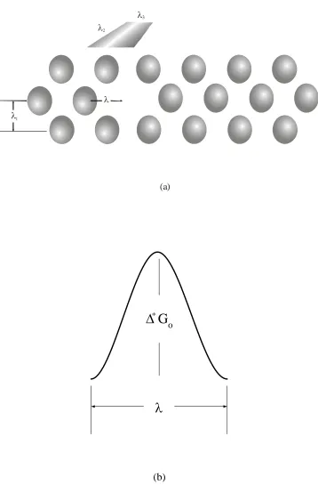
McAllister (1960) based his work on Eyring’s theory of absolute reaction rates. This theory was

established on the assumption that there are layers of molecules in the liquid and if the shear stress

is applied to a layer with the distance of 𝜆1 from the next layerthen there would be a “hole” or a

vacant site in the second layer to receive the molecule as shown in Figure 2.1(a). The availability

of this positions requires the movement of molecules from their stable positions and overcome the

potential energy barrier, ΔG*, depicted in Figure 2.1 (b). In this jump, the molecule posses a

movement frequency in the forward and backward directions calculated by the equation,

kT G

e

h

KT

r

* 0

0

∆ −

=

(2.1)

where T is the absolute temperature, K is the Boltzmann constant, and h is Planck’s constant.

In equation (2.1), if there is no force employed on the fluid then the forward and backward

(23)

λ1

λ2

λ3

λ1

(a)

λ

∆

*

G

_o

(b)

(24)

molecules in the liquid, then the molecules move in the forward and backward directions

differently. Hence, the work enforced the molecules is given,

)

2 (

3 2

λ

ε

_a

=

f

(2.2)

where f is the shear force per unit area, λ2λ3 is the average area occupied by each molecule and λ is

defined as the available space between the molecules.

If the molecule moves in the forward direction of the shear force and attain the work, εa , then the

frequency in this direction will be

)

exp(

* 0

kT

G

h

KT

r

a f

ε

−

∆

−

=

(2.3)

and correspondingly in the backward direction is as follows:

) exp( * 0 kT G h KT r a b ε + ∆ −

= (2.4)

and the net frequency is given by

( )

[

a a

]

n

kT G h

KT

r  ε − −ε

           ∆ −

= exp exp exp

*

0 _(2.5)

equation (2.5) can be rearranged to equation (2.6)

(25)

The velocity gradient between two layers of the molecules by the distance of λ1 is defined as

1

λ λr dx dv

= (2.7)

where λ is the distance per jump and r is the number of jumps per second. Since the Newton’s law

becomes as

dx dv

f =−µ (2.8)

Then by substitution of equation (2.7) into equation (2.8) yields

RT G e

h *

2 1

1

∆

= λ λ λ

λ

µ (2.9)

where ΔG* is the potential energy barrier in the form of free Gibbs energy and R is the universal

gas constant.

assuming that λ=λ1 and also λ1λ2λ3 identified as the effective volume of the molecule then equation

(2.9) converts to

RT G

m e V hN ∆ *

=

µ (2.10)

where N is Avogadro’s number and Vm is the molar volume of the liquid. In the case of kinematic

(26)

RT G

e M

hN ∆ 0

= =

ρ µ

ν (2.11)

where M is the molecular weight and ΔG0 is the molar activation energy of viscous flow.

2.2.1.1 Three-body interaction model for a binary mixture liquid system

McAllister (1960) proposed his viscosity model for binary liquid mixtures on the basis of Eyring’s

theory by equation (2.11). He assumed that if the size ratio of molecules of type 1 and 2 is less

than 1.5, then the interactions are three bodied and are all in one plane. Also, if the size ratio is

larger than 1.5, the type of interaction considered is three-dimensional four-body interaction which

means that other molecular collisions are possible. In such a case, when a molecule of type 1 with

a size ratio of 1.5 or more passes the molecular energy barrier to the available vacant area, it may

interact with molecule of type 1, type 2 or paired interaction in the presence of both situations.

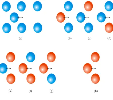
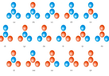
Figures 2.2 and 2.3 show types of viscosity interactions in three-body and four-body interaction

cases in a binary mixture, respectively.

In Figure 2.2, six types of possible unlike interactions in the three-body model are shown with the

classification of 1-1-1, 2-2-2, 1-2-1, 2-1-2, 1-1-2, 1-2-2. McAllister assumed that the likelihood of

each interaction is dependent on the mole fraction of each component in the mixture. Also, he

assumed that the free energy of activation is additive. On the basis of those assumptions,

(27)

(a) (b) (c) (d)

(e) _(f) (g) (h)

(28)

(a) (b) (c) (d) (e)

(l) (m) (n) (o) (p)

(f) (g) (h) (i) (j) (k)

(29)

Types of interaction 1-1-1 1-2-1 2-1-1, 2-1-2 2-2-1, 2-2-2 1-1-2 1-2-2

Fraction of total x₁3

2 2 1x x 2 2 1

2x x

2 2 1x x 2 2 1

2x x

3 2 x

occurrence

Consequently, for the mixture, the free energy of activation,∆G*_,yields

* 2 3 2 * 122 2 2 1 * 212 2 2 1 * 112 2 2 1 * 121 2 2 1 * 1 3 1 * 2

2x x G x x G x x G x G

G x x G x

G = ∆ + ∆ + ∆ + ∆ + ∆ + ∆

∆

(2.12)

Two additional assumptions made for simplicity are as follows:

* 12 *

112 *

121 G G

G =∆ =∆

∆ (2.13)

* 21 *

122 *

212 G G

G =∆ =∆

∆ (2.14)

Substitution of equation (2.13) and (2.14) into equation (2.15), results in

* 2 3 2 * 21 2 2 1 * 12 2 2 1 * 1 3 1 * 3

3x x G x x G x G

G x

G = ∆ + ∆ + ∆ + ∆

∆ _(2.15)

Although ∆G121and ∆G112are physically different, the substitutions were essential in order to

decrease the number of constants to two.

The other format of equation (2.12) can be re-written as

(

)

(

)

* 2 3 2 * 122 * 212 2 2 1 * 112 * 121 2 2 1 * 1 3 1 * 2

2 G xx G G x G

G x x G x

G = ∆ + ∆ + ∆ + ∆ + ∆ + ∆

∆ (2.16)

where

(

)

3 2 ₁₁₂*

* 121 * 12 G G

G = ∆ + ∆

∆ (2.17)

(

)

3 2 ₁₂₂*

* 212 * 21 G G

G = ∆ + ∆

(30)

Equation (2.15) specifies that for each type of energy of activation considered in this study, a

corresponding kinematic viscosity dedicated and given by

RT G

avg e M

hN ∆ *

        =

ν (2.19)

Mavg is the average molecular weight of the mixture and is expressed by

∑

=

i i i

avg xM

M (2.20)

for pure component i

RT G i i ij e M hN * ∆       =

ν (2.21)

and for interactions

RT G ij ij ij e M hN * ∆         =

ν (2.22)

where

(

)

3

2 _ij _j

ij

M M

M = + (2.23)

Substitution of equation (2.12) into equation (2.19) yields equation (2.24) for the kinematic

(31)

RT G x G x x G x x G x e M hN avg     _∆ ₊ _∆ ₊ _∆ ₊ _∆ = * 2 3 2 * 21 2 2 1 3 * 12 2 2 1 3 * 1 3 1

ν (2.24)

Taking the logarithm of equation (2.24) and omitting the free energies of activation by applying

equations (2.21) and (2.22) gives

[

]

(

)

[

]

[

(

)

]

[

2 1

]

3 2 1 2 2 2 1 1 2 2 2 1 1 2 2 1 2 3 2 21 2 2 1 12 2 2 1 1 3 1 / 3 / / 2 1 3 3 / / 2 3 / 3 3 M M n x M M n x x M M n x x M M x x n n x n x x n x x n x n          + + + + + + − + + + = ν ν ν ν ν (2.25)

The only undetermined values in equation (2.25) are the binary interaction parameters ν12 and ν21

at each temperature which can be determined by fitting the experimental data to equation (2.25)

using least-squares. The McAllister model fits a variety of experimental data and is known as the

best correlative model for the viscosities of liquid mixtures.

2.2.1.2 Extension of the McAllister three-body model to ternary liquid systems

Chandramouli and Laddha (1964) expanded McAllister’s the three-body interaction model for

viscosity of binary liquid mixtures to ternary mixtures. They assume three types of molecules with

the size ratio of less than 1.5 and three-body interactions in a plane. The proposed expression of

the kinematic viscosity of the mixture after substitutions and rearrangement is as follows:

(32)

where M1, M2 and M3 are the molecular weights of components1, 2, and 3. Moreover, there are

seven constants; six binary constants and one ternary constant. The three binary systems of

components of types 1 and 2, types 2 and 3, and 1 and 3 yield the constants ν12 andν21, ν23 and ν32,

and ν31 and ν13, respectively and a ternary constant ν123. The values of the binary constants are

determined by fitting experimental data of the viscosity of the pure components. The value of the

ternary interaction parameter is determined by fitting the experimental data using the method of

the least-squares.

2.2.1.3 Conversion of the McAllister model from a correlative to a predictive model

Despite the fact that McAllister three-body interaction viscosity model gives promising results for

calculating the viscosity of liquid mixture, it is still a correlative model and requires costly and

time consuming experimental data to obtain the values of the interaction parameters.

Asfour et al. (1991) reported a method to calculate the values of the binary interaction parameters

of binary n-alkane solutions with the use of pure component properties and molecular parameters.

Later on, Nhaesi and Asfour (1998) developed a new model for predicting the McAllister model

parameters from pure components properties of regular binary liquid mixtures. Subsequently,

Nhaesi and Asfour (2000a, 2000b) introduced a method for predicting the viscosity of

multi-component mixtures.

Asfour et al. (1991) presented a novel technique for predicting the values of binary interaction

(33)

the values of the parameters were plotted versus the corresponding temperature levels. Asfour et

al. (1991) assumed that,

(

)

1/3 2 1 1 12 ννν

ν ∝ (2-27)

Plotting the value of the lumped parameter,

( )

2 1/3 2 1 12 ν ν

ν ∝ , against the inverse of the absolute

temperature 1/T, shown in Figure 2.4, gives a horizontal line which indicates that the lumped

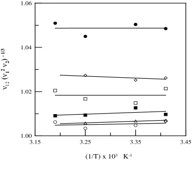
parameter is independent of temperature. Because of that, Asfour (1991) plotted the lumped

parameter versus

[

(

)

(

2

)

1/3

]

2 1 2 1

2 N / N N

N − as shown in Figure 2.5, where NA and NB are the number

of carbon atoms per molecule of component i and j. The equation of the plotted straight line is

written as:

( )

(

)

1/3

2 2 1 2 1 2 1 3 / 1 2 2 1

12/ν ν =1+k (N −N ) / N N

ν (2.28)

where k1 is the slope of the straight line and the value of that is equal to 0.044 for the systems

where N1−N2 ≤3. Equation (2.28) gives the value of interaction parameter,ν12, from pure

components properties. The value of ν21 can be computed by

(

)

1/3 1 2 12 21 ν ν /ν

ν = (2.29)

Substituting the values of interaction parameters calculated from pure components kinematic

viscosities and substituting equations (2.28) and (2.29), into equation (2.25) determines the

kinematic viscosities of the binary systems at different compositions. Consequently, this method

(34)

3.15 3.25 3.35 3.45

(1/T) x 103 K-1 1.00

1.02 1.04 1.06

ν

12

(

ν

1 2

ν

2

)

-

1/

3

Legend

Hexane (A) - Heptane (B) Hexane (A) - Octane (B) Heptane (A) - Octane (B) Heptane (A) - Decane (B) Tetradecane (A) - Hexadecane (B) Octane (A) - Decane (B)

(35)

0.00 0.40 0.80 1.20

(N2 - N1)2 (N12 N2)-1/3 1.00

1.02 1.04 1.06

ν12

(

ν1

2 ν

2

)

-

1

/3

ν ν ν₁₂ ₁2 2

1/3 2 1

2

A 2

B 2 !1/3

( ) 1 0.044(N N )

(N N )

− _{= +} −

(36)

Asfour et al. (1991) showed that in the case of liquid mixtures with N₁−N₂ ≥4, McAllister four-

body interaction model with three interaction parameters is applicable and they proposed equation

(2.30) for the calculating the value of the four-body interaction parameter, ν_iijj, exercising the

same strategy as for the three bodied model, which yields:

( )

(

₍

₎

₁

)

_/₄

2 2 2 1 2 1 2 2 4 / 1 2 2 2 1

1122/ 1

N N N N k − + = ν ν

ν (2.30)

The value of k2 , is also the slope of the straight line and the value is determined by the method of

least-squares and was found to be equal to 0.03.

The other three interaction parameters are assumed to be as follows:

( )

1/4 2 3 1 1112

ν

∝ (2.31)

( )

₂ 1/4 2 2 1 1122

ν

∝ (2.32)

( )

₃ 1/4 2 1 2221

ν

∝ (2.33)

Dividing equation (2.31) by equation (2.32) and equation (2.33) by equation (2.32) results in the

following equations:

(

)

1/4 2 1 1122 1112 ν ν /ν

ν = (2.34)

(

)

1/4 1 2 1122 2221 ν ν /ν

ν = (2.35)

Nhaesi and Asfour (1998) attempted to present the predictive form of the three-body interaction

(37)

they developed. They plotted the kinematic viscosity data of n-alkanes (C5-C20) at 308.15K versus

the corresponding carbon number of those alkanes, as depicted in Figure 2.6. The equation of the

straight line depicted in Figure 2.6 is given by,

(

)

A BN

nν_at₃₀₈_.₁₅_K = +

 (2.36)

where ν is the kinematic viscosity in cSt and N is the carbon number. The values of A and B are

-1.943 and 0.193, respectively. Later on, Al Gherwi and Asfour (2005), El-Hadad (2004) and Cai

(2004), and El-Sayed (2009) indicated that equation (2.36) tends to overpredict the values of the

effective carbon number for compounds such as cyclohexane and cyclooctane. They noted that

lower errors resulted when the ECN values obtained from equation (2.36) were multiplied by 0.75.

Nhaesi and Asfour (1998) plotted

ν

₁₂ ∝

( )

ν

₁2

ν

₂ 1/3against [(N2-N1)2/(N12N2)1/3] where Ni and Nj are

the effective carbon numbers of components and j, respectively and obtained a straight line as

shown in Figure (2.7). The equation of the straight line was obtained, by the least-square

technique, to be as follows:

( )

(

)

1/

)

3

2 2 1 2 1 2 3 / 1 2 2 1

12 ₀_.₈₇₃₅ ₀_.₀₇₁₅ N N N N − + = ν ν ν (2.37)

The value of the binary interaction,ν21, is calculated by equation (2.29).

2.2.1.4 The generalized McAllister three-body model

Nhaesi and Asfour (2000a) developed a predictive form of the generalized McAllister three-body

(38)

Figure 2.5: Kinematic Viscosity for n-alkanes versus the Effective Carbon Number (ECN)

4.00

8.00

12.00

16.00

20.00 Effective Carbon Number (ECN)

0.10

1.00

10.00 K

in

e

m

a

ti

c

V

is

c

o

s

it

y

,

c

S

(39)

parameters from the values of the viscosities of the pure components. This model includes the

binary and ternary interaction parameters similar to the three-body interaction model of ternary

systems suggested by Chandramouli and Laddha (1963).

Nhaesi and Asfour (2000a) made some assumptions to define their equation. First, they assumed

that the interactions are three-bodied and second, that the free energies of activation are additive on

a molar basis.

The activation energy of an n-component liquid mixture is given by,

∑

∑∑

∑∑∑

= = = = = = ∆ + ∆ + ∆ = ∆ n i n i n j n i n j n k ijk k j i ij j i i i

m x G x x G xx x G

G

1 1 1 1 1 1

2 3

6

3 (2.38)

The components of the mixture are i, j and k where i has the highest number of carbons and k has

the lowest.

In equation (2.38) two additional assumptions are made as follows:

ij iij iji G G G =∆ =∆

∆ (2.39)

ji ijj

jij G G G =∆ =∆

∆ (2.40)

Equation (2.41) correlates the kinematic viscosity of the mixture and ∆G is adopted from an

Arrhenius-type equation.

( G RT)

avg m

m

e M

hN ∆ /

= 

(40)

where

∑

= = n i i i

avg xM

M

1

(2.42)

for pure components i,

( G RT)

i i

i

e M hN ∆ /

= 

ν

(2.43)

for the binary interaction of type ij,

( G RT)

ij ij

ij

e M hN ∆ /

= 

ν (2.44)

where

(

2 _i _j

)

/3

ij M M

M = + (2.45)

for ternary interactions

( G RT)

ijk ijk

ijk

e M

hN ∆ /

= 

ν (2.46)

where

(

i j k

)

/3

ijk M M M

(41)

Taking the logarithm of equations (2.41), (2.43), (2.44) and (2.46) and substituting them into

equation (2.37) eliminates the free energies of activation. The following equation is the generalized

McAllister three-body model for multi-component liquid mixture:

(

)

) ( ) ( 6 ) ( 3

1 1 1 2 1 1 2 1 3 avg n i n k j i j n k ijk ijk k j i ij ij j n j i i n j i n i i i i m M n M n x x x M n x x M n x n

∑ ∑ ∑

∑ ∑

∑

= < < = = ≠ = = = − + + =      ν ν ν ν (2.48)

The kinematic viscosity of the n-component liquid mixture can be obtained from equation (2.48) if

the properties of pure components are available. The number of binary and ternary interaction

parameters depends on the components in the system. Nhaesi and Asfour (2000a) suggested the

use of equations (2.49) and (2.50) for the determination of the number of binary interactions, N2 as

well as the number of ternary interactions parameters, N3

(

2

)

! !

2 !

2 = ₋

n n

N (2.49)

(

3

)

! ! 3 ! 3 − = n n

N (2.50)

The effective carbon number and the value of the binary interaction parameters can be calculated

by following the procedure suggested by Nhaesi and Asfour (1998).

Nhaesi and Asfour (2000a) introduced a method for determining the value of ternary parameter

(42)

carbon number of each component in the mixture in the cases of n-alkane and regular liquid

mixtures, respectively; viz.,

(

)

(

j

)

i k k j i ijk N N N 2 3 /

1 0.9637 0.0313

− + = ν ν ν ν (2.51)

where i,j, and k are the components of the mixture in ascending number of carbons and Ni, Nj and

Nk are their number of carbons, respectively.

2.2.2 The pseudo-binary McAllister model

Nhaesi and Asfour (2000b) suggested the incorporation of the pseudo-binary model developed

earlier by Wu and Asfour (1992) into the generalized McAllister model for multi-component liquid

mixtures. In this way, Nhaesi and Asfour (2000b) argued that this reduces the complexity and

time taken for calculations since the pseudo-binary model reduces the number of components; no

matter how large it is, to only two. Consequently, in the pseudo-binary McAllister model, the pure

components are separated into pure component 1 and pseudo-component 2’, where component 2’

includes components 2, 3,..,n. Nhaesi and Asfour (2000b) further indicated that ternary interaction

parameters are eliminated since multicomponent liquid systems are treated as pseudo-binary

mixtures.

Nhaesi and Asfour (2000b) proposed the following series of mixing rules in order to determine the

properties of component 2’:

(

)

=

_∑

n₌

(

)

i Xi ECN i

ECN

2 '

(43)

where

∑

= = _n i i i i x x X 2 (2.53)

The molecular weight and the kinematic viscosity of the component 2’ are respectively as follows:

∑

=

= n

i Xi nMi nM2' ₂ 

 (2.54)

∑

=

= n

i Xi n i

nν2' ₂  ν

 (2.55)

2.2.3 The group contribution (GC-UNIMOD) model

Cao et al. (1992) presented a viscosity model for correlating the kinematic viscosity of pure

liquids, binary systems and afterwards predict the viscosity of multicomponent systems. Their

technique is based on statistical thermodynamics, Eyring’s absolute rate theory, and the UNIFAC

model. The kinematic viscosity equation for multicomponents is given as,

( )

=

_∑

₌

(

)

−

_∑

₌

_∑

n₌

j ji ji i i n i n i i i i

i n M qnx n

x M

n

1

ν

1

θ

τ

ν

 

 (2.56)

where M is the molecular weight of the liquid mixture, xi and Mi is the mole fraction and molecular

weight of segment i in the liquid mixture, respectively. Also, qi is the area parameter of molecule i

and ni is the proportionalityconstant of segment i calculated by equation (2.57),

∑

= = 0 j j j

i AT

n n

(44)

Where the values of Aj are correlated using the experimental data and T is the temperature of the

system.

Also, θji is the local composition parameter given by

∑

= = _n i ji ji ji i ji 1 τ θ τ θ

θ (2.58)

where τjiis the interaction parameter and θi is the average area fraction of component i in the liquid

mixture calculated by

      − − = RT U U z ji ii ji 2 exp τ (2.59)

∑

= = _n j j j i i i q x q x 1

θ (2.60)

where z is the coordination number of the lattice and is determined from the following equation

suggested by Skjold-Jorgensen (1980),

2 00014 . 0 1272 . 0 2 .

35 T T

z= − + (2.61)

Uji and Uii are the corresponding potential energies between two sites and they are temperature

dependent.

∑

=

= n

j j j

ii BT

U

(45)

In the case of binary systems, this model can correlate the viscosity data even if the data are at

different temperatures and can be predictive for multicomponent systems.

Later, Cao et al. (1993a) established a new viscosity model for the viscosity correlation and

prediction of pure and multicomponent liquids. Also, it includes a model for activity coefficients

of liquid mixtures where both the viscosity and the activity coefficients are expressed by the same

parameters. This model is called the “viscosity-thermodynamics” model (UNIMOD). The

parameters can be determined from viscosity and thermodynamic properties which are more

readily available. This method is either predictive or correlative due to derivation from

thermodynamic or viscosity data. Equation (2.63) defines the UNIMOD kinematic viscosity as

follows:

(

)

_∑

( )

∑

= = − = =      + = n

j ji ji n i i i i i n i i i i n

i i i i n

r n q x n M n M

n( ) ₁ 2 ₁ ₁ ϕ ₁θ τ

ϕ ϕ ν

ϕ

ν   

 (2.63)

where φi is the average segment fraction of component i given as

∑

=

= _n

j j j i i i r x r x 1 ϕ (2.64)

where xi is the mole fraction of the component type i given by

∑

= = _n j j i i N N x 1 (2.65)

ri is the number of segments in a molecule i which is calculated together with qi by the UNIFAC

(46)

molecular weight of component i which is acquired from the DIPPR data bank developed by

Daubert and Danner (1989).

Cao et al. (1993b) combined the group-contribution approach with the UNIMOD model and

suggested a new model called GC-UNIMOD. In this model the viscosity equation is divided into

two parts; viz., a combinatorial part and a residual part. The equation is given by,

( )

_∑

[

]

= + = n j R i C i n 1 ζ ζ ν

 (2.66)

Where ζ_iCand ζ_iRare the combinatorial and the residual parts, respectively given by

      +       = i i i i i i C i x n M M n φ φ ν φ

ζ  2  (2.67)

( )

∑

= − = n j ji i i i i i R i n r n q 1 τ φ φ

ζ  (2.68)

The residual part can also be given, using group contribution, as follows:

[

]

∑

Ξ −Ξ = ) ( ) ( ) ( k group all i ki ki i k R i ν

ζ (2.69)

Where ν_k(i)is the number of groups k per molecule of component i, Ξ_kiis the group residual

viscosity of group k for component i in the mixture and Ξ(_kii)is the group residual viscosity of

group k for component i in the solution of groups of pure liquid i.

(47)

[

]

∑

=      Ξ − Ξ +       +       = n

i allgroupk

i ki ki i k i i i i i i x n M M n n 1 ) ( ) ( 2 ) ( ν φ φ ν φ ν  

 (2.70)

where

∑

Ψ − = Ξ k group all km km i vis ki k k

mi N n

R Q ) (  θ

φ (2.71)

where Q_kis the surface area parameter of group k, R_kis the volume parameter of group k, Ψ_kmis

the group interaction parameter between group k and m, and N_kivisis the viscosity parameter of

group in component i which are calculated from equations (2.72) through (2.75)

9 10 5 . 2 x A Q wk

k = (2.72)

17 . 15 wk k V

R = (2.73)

      − ₋ − = z r r q Q

N i i i

k vis ki

1

2 (2.74)

     − = Ψ T a_km

km exp (2.75)

where a_kmis the interaction energy parameter for group k and m.

Also,

∑

= ) ( ) ( k group all k i k i Q

(48)

∑

= ) ( ) ( k group all k i k i R

r ν (2.77)

2.2.4 The generalized corresponding-states principle (GCSP) model

Teja and Rice (1981) introduced their generalized corresponding-states principle model (GCSP)

using the properties of two pure components employed in the liquid mixture as the reference and

the corresponding-state principle. The GCSP viscosity equation given as

( )

[

( )

2

( )

1

]

1 2

1

1 r r

r r r r n n n

n ηε ηε

ω ω ω ω ηε ηε     − − − +

= (2.78)

where 6 / 1 3 / 2 2 / 1 c c P T M− =

ε (2.79)

where ηε is the reduced viscosity, ω is the acentric factor of the non-spherical fluid and r1and r2

represent the reference fluids. In addition, P_cand T_care the critical pressure and temperature of the

pure components, respectively.

In case of liquid mixtures, the van der Waals one-fluid model is used to replace pure component

properties, ω, M,T_cand P_c by pseudo-critical properties, ω_m,M_m,T_cmand P_cm of the mixture

suggested by Wong et al. (1983) as follows

(

)

=

_∑∑

(

)

i j i j cij cij cm

cm P xx T P

T2 / 2 /

(2.80)

(

)

=

_∑∑

(

)

i j i j cij cij cm

cm P xx T P

(49)

(

cm cm

)

_i _j i j

(

cij cij

)

ij

m T P xx T P ω

ω 2/3

/

/ =

∑∑

(2.82)

where

(

)

1/2

cjj cii ij cij T T

T =ξ (2.83)

where

ξ

is the binary interaction parameter; and set one if the GCSP method is predictive.

(

)

1/3

[

(

)

1/3

(

)

1/3

]

/ /

2 1

/ _cij _cii _cii _cjj _cjj

cij P T P T P

T = + (2.84)

(

ii jj

)

ij ω ω

ω = +

2 1

(2.85)

When the values of pseudo-critical properties are substituted in equations (2.78) and (2.79), one

obtains the kinematic viscosities of the multicomponent liquid mixture.

2.3 The Empirical Models for Predicting the Viscosities of Liquid Mixtures

2.3.1 The Allan and Teja correlation

Allan and Teja (1991) presented a method for the prediction of the viscosity of hydrocarbons based

on data for the normal alkanes. They suggested the use of an Antoine-type equation which

correlates the viscosity and the temperature of liquids, as follows:

(

)

[

B T C

]

A

nµ= −1/ +1/ +

 (2.86)

(50)

B

A, , and Care constants calculated using the liquid viscosity data between ambient pressures and

saturation pressures. The correlation of the number of carbon atoms of n-alkanes by fitting liquid

viscosity data together gives the following equations:

A=145.73+ 99.01n+ 0.83n2- 0.125n3 (2.87)

B= 30.48+34.01n-1.23n2+0.017n3 (2.88)

C= -3.07- 1.99n (2.89)

where n is the carbon number of the mixture which is calculated with the help of the following

mixing rule:

∑

=

= n

i i i

m xN

N

1 (2.90)

In order to determine the viscosity of hydrocarbon mixture, the composition and the carbon

number of pure components should be known. The mixture data are not required in this model

which makes it predictive and easier to use.

The main deficiency of the Allan and Teja correlation according to Gregory (1992), is that the

results for the carbon numbers greater than 22 contain errors.

2.3.2 The Grunberg and Nissan mixture law for viscosity

The methods to estimate or correlate the viscosity of liquid mixture assume that the viscosity of the

pure components of the mixture is known. In 1887, Arrhenius proposed his method for predicting

(51)

2 2 1

1log log

logη=x η +x η (2.91)

Where η is the viscosity of the binary solution and x₁and x₂are the mole fractions and η₁and η₂

are viscosities of components 1 and 2, respectively.

Grunberg and Nissan (1949) believed there are positive and negative deviations occurring during

working with Arrhenius equation. For that reason they proposed an applicable equation which is

more accurate except in case of aqueous solutions. They suggested an Arrhenius-type and low

temperature viscosity equation with the application of vapor pressures and viscosities of solutions

for correlating the viscosity data of binary solutions given as

12 2 1 2 2 1

1log log

logη_m =x η +x η +xx G (2.92)

where G12 is an interaction parameter which is a function of the components 1 and 2 as well as the

temperature. The value of G₁₂ is calculated by plotting the viscosity of the system η_m versus the

liquid mole fraction 1,

( )

x₁ . The value Greported by Grunberg and Nissan (1949) for the

trans-decalin and cis-trans-decalin is - 0.0224 and it gave promising results when used with the data collected

by Bird and Daly (1939). Grunberg and Nissan (1949) showed that the interaction parameter can

assume negative and positive values in the case of positive and negative deviations from Rault’s.

Margules (1895) proposed equation (2.93) to calculate G₁₂by using the constant valueb, given by

G12=C.b (2.93)

(52)

logγ1 2 2 bN

= (2.94)

Whereas γ1 is the activity coefficient of component 1 and C is the ratio of viscosity to the

logarithm of vapor pressure which always takes a negative value.

Later, Irving (1977) presented an equation for multi-component mixtures based on Grunberg and

Nissan (1949) equation as follows:

∑ ∑

∑

= + = =

= n

i n

j i j ij i

n i i

m x n xx G

n

1 1

1

η



 (2.95)

(53)

CHAPTER 3

EXPERIMENTAL PROCEDURES AND EQUIPMENT

3.1 General

This chapter presents the procedure of solution preparation, the determination of density and

viscosity of the multicomponent liquid mixtures including binary, ternary, quaternary and quinary

systems. Also, it contains the results of the verification of the purity of the chemicals used in

composing the solutions and those used for the calibration of the density meter.

3.2 Materials

The chemicals used in this study are divided into two groups. The first group contains the

chemicals that were used in calibrating the density meter and the viscometer. The second group

contains the chemicals that were used in composing the systems of interest in the present study.

The calibration fluids used in calibrating the viscometers were purchased from Cannon

Instruments Company. The calibration fluids employed in calibrating the density meter were:

ethylbenzene, nitrobenzene, 1-butanol, 1-nonanol and deacane. The chemicals employed in

preparing the liquid mixtures include: cyclohexane, p-xylene, chlorobenzene, propanol and

1-octanol.

The manufacturer’s stated purity of the chemicals employed in composing the liquid systems were

+99%. The stated purities were verified by means of gas chromatographic analysis. Table 3.1 lists

the stated purity of chemicals as well as the purities as determined by gas chromatographic

(54)

Table 3.1: Gas Chromatography Analysis Results of the Pure Components

Compound Manufacturer Stated Purity

mol %

GC Analysis mass %

p-Xylene Sigma - Aldrich 99+ 99.98

Chlorobenzene Sigma - Aldrich 99.8 99.99

Nitrobenzene Sigma - Aldrich 99+ 99.85

Cyclohexane Aldrich 99+ 99.69

Ethylbenzene Sigma - Aldrich 99.8+ 99.98

1-Propanol Sigma - Aldrich 99.5+ 99.88

1-Butanol Sigma - Aldrich 99.8+ 99.89

1-Octanol Sigma - Aldrich 99+ 99.98

(55)

3.3 Preparation of Solutions

In order to prepare the samples, the volume of each component estimated by a computer program

and injected into clean and dried 30 mL glass vials. First, each glass vial was sealed by Tuf-bond

(Silicon-Teflon) discs where the Teflon side faces the solution in order to prevent the chemical

reactions and the silicon side minimizes the evaporation of the volatile contents after puncturing

the disc by a syringe. An aluminum cap is placed on the disc so that the disc is retained.

A Mettler HK 160 electronic balance with a precision of ± 1 x 10-7 kg was used for weighing the

vials when they are empty and after injection of each component. After composing the solutions

the vials were kept in the refrigerator until the time of measurements.

3.4 Density Measurements

The densities of the calibration chemicals, pure components, and samples were measured at

293.15 K and at 298.15 K by an Anton-Paar DMA 60/602 density meter unit that contains a

U-tube shaped hollow oscillator. The density meter is placed in a temperature controlled wooden

chamber that was designed by Asfour (1980). The wooden chamber and the density meter with the

temperature control system are shown in Figure 3.1. The frequency variation in the DMA 602

oscillator is monitored by the DMA 60 processing unit and displayed on the digital screen as six

digits values in seconds. The frequency alters due to changes in the sample mass and the

temperature during the process. Equation (3.1), provided by the manufacturer, was used to

calculate the density from the density meter readings:

C BT AT ₋

−

= 2 ₂

1

(56)

where

ρ

is the density and T is the period of oscillation, in seconds, shown by the density meter.

A,B, and C are adjustable parameters that were determined by fitting the well-known density

values of the calibration fluids with their corresponding density meter readings using least-squares.

The density meter is placed in a wooden chamber accessed through a plastic removable cover. The

chamber heats up with the electrical bulbs placed inside the chamber to reach the desired

temperature. An Omega precision thermometer equipped with a calibrated ITS-90 platinum probe,

with the precision of ±0.005 K, monitored the temperature inside the density meter. The density

meter’s measuring cell was flushed with ethanol and dried by blowing dry air into the cell. After

each injection, the sample was kept to between 15 to 20 minutes to reach thermal equilibrium

(57)