University of Windsor University of Windsor
Scholarship at UWindsor
Scholarship at UWindsor
Electronic Theses and Dissertations Theses, Dissertations, and Major Papers
2014
Demographic Obesity Modeling Based on Complex System
Demographic Obesity Modeling Based on Complex System
Dynamics
Dynamics
Farzaneh Salamati
University of Windsor
Follow this and additional works at: https://scholar.uwindsor.ca/etd
Recommended Citation Recommended Citation
Salamati, Farzaneh, "Demographic Obesity Modeling Based on Complex System Dynamics" (2014). Electronic Theses and Dissertations. 5180.
https://scholar.uwindsor.ca/etd/5180
This online database contains the full-text of PhD dissertations and Masters’ theses of University of Windsor students from 1954 forward. These documents are made available for personal study and research purposes only, in accordance with the Canadian Copyright Act and the Creative Commons license—CC BY-NC-ND (Attribution, Non-Commercial, No Derivative Works). Under this license, works must always be attributed to the copyright holder (original author), cannot be used for any commercial purposes, and may not be altered. Any other use would require the permission of the copyright holder. Students may inquire about withdrawing their dissertation and/or thesis from this database. For additional inquiries, please contact the repository administrator via email
Demographic Obesity Modeling Based on Complex System Dynamics Approach
by
Farzaneh Salamati
A Thesis
submitted to the Faculty of Graduate Studies
through the Department of Industrial and Manufacturing Systems Engineering
in Partial Fulfillment of the Requirements for
the degree of
Master of Applied Science
at the University of Windsor
Windsor, Ontario, Canada
2014
Demographic Obesity Modeling Based on Complex System Dynamics Approach
by
Farzaneh Salamati
APPROVED BY:
Dr. R. J. Caron
Department of Mathematics & Statistics
Department of Industrial and Manufacturing Systems Engineering
(Cross Appointed)
Dr. N. Zamani
Department of Mechanical Automotive & Materials Engineering
Dr. Z. J. Pasek, Advisor
Department of Industrial and Manufacturing Systems Engineering
iii
DECLARATION OF PREVIOUS PUBLICATION
This thesis includes an original paper that has been previously published for publication in peer reviewed journals, as follows:
Thesis Chapter Publication title/full citation Publication status*
Chapter 1 Salamati, F., Pasek, Z. J. (2013). Personal Wellness: Complex and Elusive Product and Distributed Self-Services. 13th International Conference on Grand Challenges in Modeling & Simulation
published
I certify that I have obtained a written permission from the copyright owner(s) to include
the above published material(s) in my thesis. I certify that the above material describes
work completed during my registration as graduate student at the University of Windsor.
I declare that, to the best of my knowledge, my thesis does not infringe upon anyone’s
copyright nor violate any proprietary rights and that any ideas, techniques, quotations, or
any other material from the work of other people included in my thesis, published or
otherwise, are fully acknowledged in accordance with the standard referencing practices.
Furthermore, to the extent that I have included copyrighted material that surpasses the
bounds of fair dealing within the meaning of the Canada Copyright Act, I certify that I
have obtained a written permission from the copyright owner(s) to include such
material(s) in my thesis.
I declare that this is a true copy of my thesis, including any final revisions, as approved
by my thesis committee and the Graduate Studies office, and that this thesis has not been
iv
ABSTRACT
The aim of this thesis is development of a systemic obesity model that can track and
monitor body weight on individual and population levels.
Considering that obesity is responsible for over 60% of all leading death causes in
developed societies and the world-wide spread of that preventable condition, it is critical
to understand the mechanisms that may lead to its control and containment. The obesity
model presented here was developed using System Dynamics (SD) approach which helps
to map complex and dynamic causal relations, containing multiple feedback loops,
between key variables and their effects and also considered in the temporal domain.
The model is validated by using the actual data provided by a Windsor Medical Weight
Loss Clinic in Windsor, ON, and actual data acquired from online sources. Based on the
available data, sensitivity analysis was performed, as well as a variety of scenario
v
DEDICATION
I would like to dedicate my thesis with all my heart to my beloved family,
to my mother, for her unconditional support of mystudies and giving me a chance
to prove and improve myself through all walks my of life, and
to my brother who has never left my side and supported me each step of the way,
vi
ACKNOWLEDGEMENTS
It is with immense gratitude that I acknowledge the support and help of my thesis
adviosor Dr. Zbigniew J. Pasek. His sage advice, insightful criticisms, and patient
encouragement aided the writing of this thesis in innumerable ways. I wish to thank my
committee members Dr. Nader Zamani and Dr. Richard J.Caron for sharing their
expertise and precious time. I would also like to thank Marzieh Mehrjoo and Mahdieh
Najafi for their technical support. Also, I would like to thank all of my friends who
vii
TABLE OF CONTENTS
DECLARATION OF PREVIOUS PUBLICATION ... iii
ABSTRACT ... iv
DEDICATION ... v
ACKNOWLEDGEMENTS ... vi
LIST OF TABLES ... ix
LIST OF FIGURES ... xi
LIST OF ACRONYMS ... xiii
CHAPTER 1 INTRODUCTION ... 1
1.1. Background & Motivation ... 1
1.1.2. Understanding Obesity... 7
1.2. Problem Statement ... 9
1.3. Proposed Approach ... 10
1.3.1. System Dynamics... 11
1.3.2. Some Main Features of Systems Dynamics... 11
1.3.3. SD’s Essential Differentiators ... 11
1.3.4. Feedback Thinking... 12
1.3.5. Loop Dominance and Nonlinearity ... 12
1.3.6. The Endogenous Point of View ... 12
1.3.7. System Structure ... 12
1.3.8. Behavior as a Consequence of Structure ... 13
1.3.9. Levels and Rates ... 13
CHAPTER 2 LITERATURE REVIEW ... 15
2.1. Body Weight Modeling ... 15
2.2. Obesity System Modeling ... 17
2.3. Key Modeling Causal Relationships ... 18
viii
2.5. Asymptotic Approach to Steady State ... 21
2.6. Constant Rate of Weight Gain ... 22
2.7. Issues and Misconceptions about Obesity ... 25
2.8. Modeling Tools ... 27
2.9. Causal Relationships and Standards ... 28
2.10. Social Networks Can Affect Weight ... 29
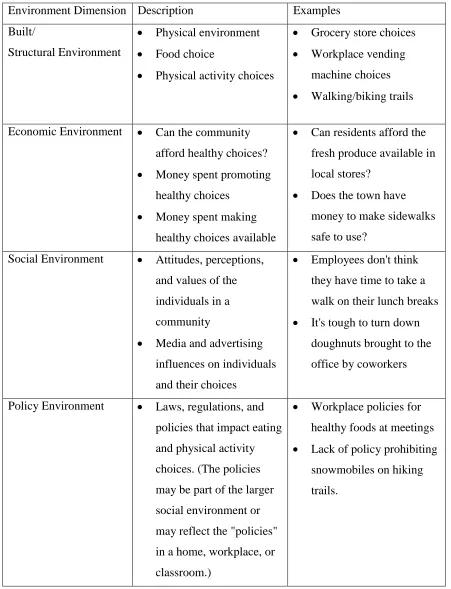
2.10.1. Obesogenic Environments ... 31
2.10.2. Environmental Effects on Obesity ... 31
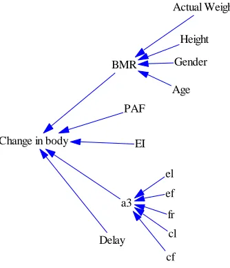
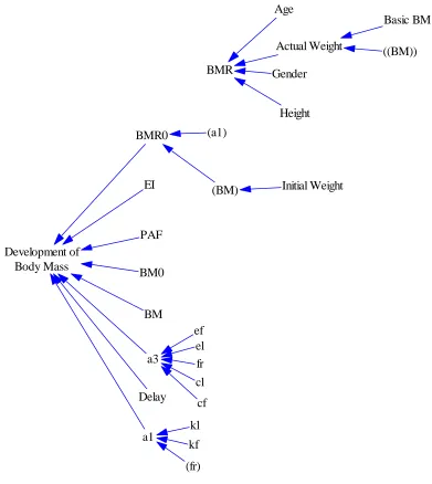
CHAPTER 3 THE INDIVIDUAL-LEVEL MODEL... 35
3.1. Model Structure and Definition... 35
3.2. Formulas Used in the Model ... 38
3.3. How the Model Can Be Used in Policy Intervention ... 40
CHAPTER 4 POPULATION-LEVEL MODEL ... 41
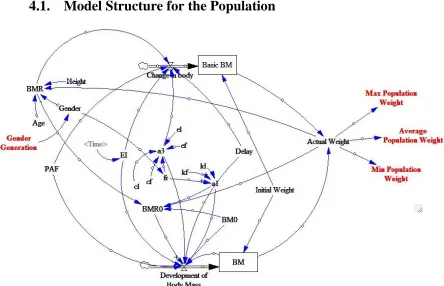
4.1. Model Structure for the Population ... 41
4.2. The formula used in the model for population ... 42
CHAPTER 5 MODEL VALIDATION AND SCENARIOS FOR BOTH INDIVIDUAL AND POPULATION LEVEL ... 44
5.1. Model Validation... 44
5.2. Comparative Analysis ... 45
5.3. Overeating Scenario for the Population Level Model ... 46
5.4. Two-day a Week Fasting Scenario... 48
CHAPTER 6 REGRESSION AND SENSITIVITY ANALYSIS ... 51
6.1. Regression Analysis ... 51
6.2. Monte Carlo Simulation ... 58
CHAPTER 7 LIMITATIONS AND FUTURE WORK ... 66
Appendix A ... 67
REFRENCES ... 72
ix
LIST OF TABLES
Table 1-1 – Weight Categories………...4
Table 1-2 – Death causes (thousands) attributable to risk factors in Canada………..6
Table 2-1– PA categories for men……….16
Table 2-2– PA categories for women………....17
Table 2-3– Physical activity categories……….17
Table 2-4– Major software Packages for SD Modeling………...……….26
Table 2-5 – Dimensions of environment………...………32
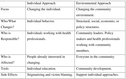
Table 2-6 – Differences between individual and environmental approaches to obesity prevention………..…34
Table 6-1 – Characteristics of standard male and female………..51
Table 6-2 – Weight for a standard male at the 30th day for specific amount of EI and PAF………52
Table 6-3 – Regression Statics for a standard male……….………..…53
Table 6-4 – ANOVA for standard male……….53
Table 6-5 – Weight for a standard female at the 30th day for specific amount of EI and PAF………....54
Table 6-6 – Regression Statics for standard female………...…55
Table 6-7 – ANOVA for standard female………..55
Table 6-8 – Ratio of 0.5626EI/4.1082PAF for standard male………...56
Table 6-9 – Ratio of 0.5171EI/2.9689PAF for standard female………56
Table 6-10 – Sensitivity Scenario………..59
Table A-1 – Weekly recording of the actual and simulated weight for a 39 year-old male who is 160 cm tall………..………67
x
Table A-3 – Probability output for a standard male………..69
Table A-4 – Residual output for a standard female………...……70
xi
LIST OF FIGURES
Figure 1-1 – Growth of Canadian population vs. Healthcare Spending 2000 – 2008…….1
Figure 1-2 – Healthcare Costs associated with obesity………..….2
Figure 1-3 – Forecast of future prevalence of adult obesity in Canada………...3
Figure 1-4 – Percentage distribution of household population………4
Figure 1-5 – Future forecasts for the three main indicators of government health expenditures ………...……….5
Figure 2-1 – Human body energy balance principle….……….... 18
Figure 3-1 – Obesity System Model for an Individual………..35
Figure 3-2 – Section I Structure……….36
Figure 3-3 – Section II Structure ……….…….36
Figure 3-4 – Section III Structure ……….…37
Figure 4-1 – Obesity System Model for a Population……….……..41
Figure 5-1 – Ten-year simulation for a 20 years old female………..45
Figure 5-2 – Weight simulation for a 39 year-old male……….………46
Figure 5-3 – Average population weight due to overeating……….………….47
Figure 5-4 – Minimum, Maximum and average population weight due to overeating….47 Figure 5-5 – Comparison of average population weight with energy intake………….…48
Figure 5-6 – Average population weight due to two days fasting in a week……….49
xii
Figure 5-8 – Average population weight when EI has been increased in two-day fasting
scenario………..50
Figure 6-1 – Relation between EI, PAF and Weight for a standard male……….52
Figure 6-2 – Relation between EI, PAF and Weight for a standard female………..54
Figure 6-3 – Relation between EI, PAF and ratio of 0.5626EI/4.1082PAF for standard male………56
Figure 6-4 – Relation between EI, PAF and Ratio of 0.5171EI/2.9689PAF for standard female……….……57
Figure 6-5 – Average Population Weight at EI = 8.37 MJ/d & PAF = 1.375……..…….59
Figure 6-6 – Sensitivity EI with Maximum Range and Variation……….60
Figure 6-7 – EI Small Range/Maximum Variation………61
Figure 6-8 – EI Maximum Range/Small Variation………61
Figure 6-9 – PAF with Maximum Range and Variation………62
Figure 6-10 – PAF Small Range/High Variation………..…….63
Figure 6-11 – PAF Large Range/Small Variation………...63
Figure 6-12 – EI & PAF Both Maximum………..…64
Figure 6-13 – EI & PAF Both Minimum………..….64
Figure 6-14 – EI & PAF Minimum Variation………...65
xiii
LIST OF ACRONYMS
BEE Basal energy expenditure
BM Body Mass
BM0 Reference Body Mass
BMss Steady State Body Mass for constant EI and PAF
BMI Body Mass Index
BMR Basal Metabolic Rate
BMR0 Basal Metabolic Rate at BM0
BMss Steady state body Mass
BW Body weight
C Total content of combustible energy in body
Energy stored per kilogram fat
Energy stored per kilogram lean tissue
DES Discrete Event Simulation
Distr Distribution
EE Energy Expenditure
EEc Energy Expenditure used to convert excess energy into tissue
EI Energy Intake
EIss Steady State energy intake for given body mass and FAP
Efficiency in the conversion of energy to fat mass
Efficiency in the conversion of energy to lean mass
Fig Figure
xiv
FM Fat Mass
Fraction of Fat
GHEX Government Health Expenditure
Basal metabolic rate per kilogram fat
Basal metabolic rate per kilogram lean tissue
LM Lean Mass
Max Maximum value used from upper side of the range
Mean Average value used for generating the date
Min Minimum value used from the lower side of the range
NCDs Non-Communicable Diseases
NPF Non-Physical Factor
OAREV Available Own Source Revenue
PA Physical activity
PAL Physical Activity Level
PAF Physical Activity Factor
RMR Resting Metabolic Rate
RN Random Normal
SD System dynamics
TAREV Total Available Revenue
TEE total energy Expenditure
Var Variation
W Weight
1
CHAPTER 1
INTRODUCTION
1.1.
Background & Motivation
In the first decade of the 21st century Canada’s population increased almost 5% from 31 million to more than 33 million (see Figure 1-1). At the same time, total personal
spending on medical care and healthcare services grew by more than 70% from $29
billion to $38 billion from 2000 to 2004 and then exceeding the $50 billion threshold in
2008 (Statistics Canada, 2010).
Figure 1-1 – Growth of Canadian population vs. healthcare spending 2000-2008.
If health care costs continue to grow at that rate, healthcare spending will soon
overwhelm provincial and federal budgets (Statistics Canada, 2010). Such a predicament
is common to many countries, independent of their economic development level.
Effective working solutions, however, despite vigorous national discussions, have not yet
been found. To prevent this from happening, many governments are implementing hard
cost control measures, which effectively use various forms of health care rationing, either
by limiting access to the health care system (in the US approximately 17% of population
2
have set budget limits for annual health expenditures, which in turn creates waiting lines
for elective procedures). The root causes of continuous cost increases in health care are
many: demographic trends, expanding longevity and quality of life, new technologies,
insurance bureaucracy overhead, etc. While there are many reasons for growing demand
for health services, the situation is exacerbated by the corresponding escalating costs;
reasonable solutions are unfortunately not yet apparent (Salamati & Pasek, 2013).
The growing demand for health services is also an expression of a global trend in which
increasing part of the population is afflicted by various chronic conditions and
non-communicable diseases (NCDs), which can be managed and are not necessarily fatal. In
fact, according to WHO in 2005 over 60% of deaths worldwide were attributable to
NCDs, but by 2020 that number is expected grow by 70%. NCDs are also often referred
to as ―lifestyle‖ diseases (or ―diseases of the rich‖) because most of them are caused by
smoking, alcohol abuse, poor diets and physical inactivity, etc. and, in principle, are
preventable. Two of the leading NCDs, cardiovascular disease and diabetes, have a very
strong causal link to obesity (White, 2001).
Figure 1-2 – Healthcare costs associated with obesity (BusinessWeek, June 10, 2007)
The spreading prevalence of obesity among workforce impacts employers’ health-care
costs due to the medical problems associated with obesity (see Figure 1-2). According to
+20%
3
a Thomson Healthcare survey of 54,000 employees, healthcare spending for a severely
obese employee can be even 75% higher than that on an employee of normal weight. The
occurrence of circulatory and metabolic diseases such as diabetes is three times higher in
obese workers, who also exhibit more instances of arthritis, back pain, and are more
prone to injuries (Bloomberg Business Week Magazine, June 10, 2007).
Another side effect of overweight/obesity is discrimination against people with weight
issues, which is a result of a popular negative stereotype that overweight/obese
individuals are inactive, uninspired or lacking strong-mindedness. Such an image causes
remarkable injustice in employment, health, health care and education (Canadian Obesity
Network).
Figure 1-3 shows predictions of future prevalence of adult obesity in Canada from 2013
to 2019, by weight category. It is estimated that by 2019, 55.4% of the adult population in
Canada will be overweight (34.2%) and obese (21.2%). In addition, the prevalence for
obese classes I, II and III is expected to increase to 14.8%, 4.4% and 2.0%, respectively
(Twells, et al., 2014).
Figure 1-3 - Forecasts of future prevalence of adult obesity in Canada
The World Health Organization (WHO) developed guidelines for evaluating obesity
4
of the practical recommendations for fighting obesity based on (Lau, Douketis, Morrion,
Hramiak, & Sharma, 2007). The common way to classify adults is based on calculation
of Body Mass Index (BMI) derived from weight and height data (Ko & Tang, 2007),
using the following formula:
(1-1)
Table 1-1 - Weight Categories
Category BMI Category BMI
Normal 18.5–24.9 Obese class I 30.0–34.9
Overweight 25.0–29.9 Obese class II 35.0–39.9
Obese ≥ 30.0 Obese class III ≥ 40.0
Figure 1-4 - Percentage distribution of household population aged 18 or older, by body
mass index (BMI), Canada excluding territories, 1978/79 and 2004 (1978/79 Canada
Health Survey; 2004 Canadian Community Health Survey: Nutrition).
It is estimated that direct costs of overweight and obesity stand at $6 billion – 4.1 % of
Canada’s total current health care budget. However, this estimate only captures health
care costs directly related to obesity, and does not represent indirect effects, such as, for
5
10-year projection for the three main indicators of Government Health Expenditures
(GHEX), Own Source Revenue (OAREV) and Total Available Revenue (TAREV) is
shown in Figure 1-5 (Rovere & Skinner, 2010). All show alarming trends. These
projections demonstrate that if Ontario does not significantly restructure the way it
finances healthcare spending, then these expenditures will devour 75% and 100% of the
Province’s own-source revenue by 2019 and 2030, respectively. Thus it is imperative that
agencies responsible for population’s health (e.g., government, health care systems, etc.)
introduce right health policies, initiatives and take appropriate actions.
Figure1-5 - Future forecasts for the three main indicators of government health
expenditures (Rover & Skinner, 2010)
Obesity is commonly recognized as a condition leading to many other medical
conditions. It is responsible (directly or indirectly) for over 60% of all leading death
causes in developed societies, not to mention significant contribution to the health care
costs (Bhattacharya, 2011).
Table 1-2 shows the impact of preventable diseases in relation to the population mortality
rates (Danaei, et al., 2009) and gives all-cause deaths (thousands) attributable to risk
6
As can be readily noted, tobacco smoking and high blood pressure are two leading death
causes in Canada among both men and women. Overweight – obesity and physical
inactivity, together, are the second most frequent death causes after tobacco smoking. By
considering indirect impact of obesity (e.g., high blood pressure, high glucose, dietary
trans-fatty acids, etc.) the impact can be even greater. Furthermore, overweight and
obesity increase the risk of many preventable diseases such as cardiovascular disease,
hypertension, type-2 diabetes, arthritis and some types of cancer (World Health
Organization, 2003; Wannamethee, 2005).
Table 1-2 – Death causes (thousands) attributable to risk factors in Canada
Risk Factor Male Female Both Sexes
Tobacco smoking 248 (226-269) 219 (169-244) 467 (436-500)
High blood pressure 164 (153-175) 231 (213-249) 395 (372-414)
Overweight-obesity (high BMI)
114 (95-128) 102 (80-119) 216 (188-237)
Physical inactivity 88 (72-105) 103 (80-128) 191 (164-222)
High blood glucose 102 (80-122) 89 (69-108) 190 (163-217)
High LDL cholesterol 60 (42-70) 53 (44-59) 113 (94-124)
High dietary salt (sodium) 49 (46-51) 54 (50-57) 102 (97-107) Low dietary omega-3 fatty
acids (sea food)
45 (37-52) 39 (31-47) 84 (72-96)
High dietary trans fatty acids
46 (33-58) 35 (23-46) 82 (63-97)
Alcohol use 45 (32-49) 20 (17-22) 64 (51-69)
Low intake of fruits and vegetables
33 (23-45) 24 (15-36) 58 (44-74)
Low dietary polyunsaturated fatty acids (PUFA)(in replacement of SFA)
9 (6-12) 6 (3-9) 15 (11-20)
Even though obesity has been well studied from the medical outlook of an individual,
there is still a need for understanding the causes and effects from systemic point of view.
The system in this case pertains to both individual (human body) level and population
7
The focus of the work presented in this thesis is on development and testing of an obesity
system model representing an individual, which is also explored on a range of conditions
of a population.
1.1.2.
Understanding Obesity
While a multitude obesity related research results is being published every year, these
efforts are generally not coordinated and focused, and they typically lead to only
fractional models addressing some narrow aspect of the phenomena. Even though the
global spread of obesity is being acknowledged, no successful efforts to fight it have been
developed. As (Lustig, 2006) pointedly described it: ―The Centers for Disease Control
and Prevention says obesity results from an energy imbalance, by eating too many
calories and not getting enough physical activity. Big Food says it’s a lack of activity, the TV industry says it’s the diet. The Atkins people say it’s too much carbohydrate, the Ornish people say it’s too much fat. The juice people say it’s the soda, the soda people say it’s the juice. The schools say it’s the parents, the parents say it’s the schools. How are we going to fix this, when no one will accept responsibility?‖
One of the key reasons for that is limited understanding of those phenomena. Most of the
contemporary obesity mechanism models are based either on glucostatic theory (Mayer
1953) or lipostatic theory (Kennedy 1953). Based on either of those theories the origin of
obesity is perceived as a disorder in one of the two feedback systems (e.g., signaling
equilibrium of either fat deposition or glucose blood levels). In practice, however, neither
of those two approaches could satisfactorily explain the obesity phenomenon (Salamati &
Pasek, 2013).
The basic logic for body weight equilibrium can be explained as follows: if the energy
intake (EI) from different sources of food (both solid and liquid) exceeds the total energy
expenditure (TEE) due to resting metabolic rate (RMR), energy used to digest food, and
physical activity (PA), then the individual will gain weight, otherwise individual loses
weight or maintains the current weight if EI = TEE.
Several factors complicate dynamic modeling of weight change. First, RMR is a function
8
(FFM)), gender, race, and age (Harris & Benedict, 1919; Cunningham, 1980; Bernstein,
Thornton, et al., 1983; Schofield, 1985; Cunningham 1991; Bitar, Fellmann, et al., 1999;
Frankenfield, Roth-Yousey, et al., 2005). Variation in EI affects RMR as well the
adaptive thermogenesis process (Rosenbaum, Leibel et al., 1997; Jequier & Tappy, 1999;
Rosenbaum, Hirsch, et al., 2008). Moreover, obesity is traditionally defined by body
mass index (BMI), which considered by many researchers not the most reliable
indicator..
(Poehlman, 1992) found that ―total daily energy expenditure and its components decline
with advancing age. However, (Speakman & Westerterp, 2010) discovered that in the
first half of life it increases with age, but in the second part of life (>57.8 for men and
>39.8 for women), RMR is decreasing with age. However, in many statistical studies, age
is treated as an independent variable in explaining RMR (Harris and Benedict 1919;
Cunningham 1980; Cunningham 1991; Vaughan, Zurlo et al. 1991; Poehlman 1992;
Maffeis, Schutz et al. 1993; Tershakovec, Kuppler et al. 2002; Speakman & Westerterp,
2010). The model distinguishes individuals based on age, gender, height, initial weight
and takes physical activity and energy intake as inputs and provides the dynamics of body
weight as outputs.
In considering weight, food (solid and liquid) consumption is the most important source
of daily energy intake by an individual. Whether individuals’ energy intake is provided
by various food categories, such as carbohydrates, fats, or proteins, the impact on
dynamics of weight is not significantly different as long as the number of caloric intake
stays the same. Thus, the main emphasis in this study is on the total EI and there are no
differences between different nutrients are considered to have significant effects
(Rahmandad & Sabounchi, 2011).
Factors associated with energy expenditure are more varied. These factors include either
the resting metabolic rate or basal metabolic rate (RMR: the energy needed to perform
essential body tasks while body is at rest) which account for 50-75% of energy
expenditure, the energy used for physical activity, and the energy used to digest
consumed food and nutrients and creation of new tissue. RMR is dependent on the body
9
differences between individuals such as age, and gender. Energy spending associated
with physical activity (PA) is largely proportional to the total weight (BW~FM+FFM)
and the PA severity (Rahmandad & Sabounchi, 2011).
1.2.
Problem Statement
The aim of this research is to develop a dynamic model of individual/population weight
change over time which eventually will lead to development of useful rules for body
weight management and control (both on individual and population levels). The model
can be used at the single individual level and be very useful for tracking and management
of the body weight as a function of individual physical and environmental attributes,
energy intake, and physical activity levels. Taking into account the same categories and
applying them to a population (e.g., by using proper distributions of parameters and
variables), model can also provide insights into similar population-wide responses. The
population level analysis is of particular importance to institutions responsible for public
health (e.g., governments, health care systems, etc.) and their long-term efforts to
maintain both healthy populations and control health-related expenditures at the same
time.
The model, based on available medical literature and data is intended as a decision
support tool assisting decision makers in exploring long-term effects of the policies they
may consider developing and implementing. Policies are defined as principles or
protocols to guide decisions leading to achieve rational outcomes. In terms of population
health advocacy for ―healthy‖ public policies is not enough, it also has to be supported by
corresponding preventive measures (in particular when dealing with response to
diseases), meaning that stewards of public health must develop and explore variety of
options for disease control and prevention. It is also worth noting that obesity was
recognized as a disease by American Medical Association (AMA) only last year (2013).
On the other hand, obesity is still not well understood, and as a result models to represent
10
1.3.
Proposed Approach
The target of this research is to study the time-based dynamics of obesity to create a
reliable system dynamics model that can be used for obesity policy analysis at population
level. The model has two-levels. The presented model is based on individual level energy
models which allow to explore the weight change over the individuals’ life, and further
extends individual level model to the population level. The model captures individual
characteristics, such as, gender, height, initial weight, and age and uses physical activity
and energy intake as inputs to provide the time-varying body weight as output. In this
study the body weight dynamics on individual level model will be introduced first and
then the population level model, consisting of multiple replications of individual models
and their relationships will be discussed (Rahmandad & Sabounchi, 2011).
According to (Collins, Khoury, Morton, & other, 2008) the most common forms of
obesity are dependent on a number of factors or causes such as genes and environment,
including diet and physical activity patterns. Genetics plays an indispensable part in
energy homeostasis and influences energy intake and spending, and further partitioning
of calories, which include tendency to store calories ingested when they exceed the actual
energy expenditure (Chung, 2008). Another effect of genetic variations is visible in
eating behavior, taste, and fullness (Rankinen, Bouchard, 2006, Wardle, Carnell,
Haworth, et al., 2008). Furthermore, "obesogenic" environment provides plenty of
opportunities to increase energy intake (e.g., increased availability and access to fast food
outlets) and reduce availability of physical activity (e.g., fewer physical activity
opportunities due to lack of sidewalks, walking trails, bike lanes, or parks).
The system proposed in this thesis accounts for the differences among individuals. This
means that not only the physical but also the non-physical factors (both endogenous and
exogenous) differences need to be considered (Collins, Khoury, Morton, & Olster, 2008).
Development of the model is based on the assumption that each individual is an
independent entity with different characteristics of age, gender, height, weight, food
consumption and physical activity patterns. It is impossible to find even two individuals
11
1.3.1.
System Dynamics
System Dynamics (SD) is a perspective and set of conceptual tools to understanding how
complex systems behave over time (Sterman, 2000). This modeling approach is often
used to simulate complex systems for policy analysis and design (Michael, Radzicki,
Robert, & Taylor, 2008). The main difference between System Dynamics and other
approaches is dealing with internal feedback loops, stocks, and flows. These elements
shows that even simple systems may behave in a complex nonlinearity way‖ (System
Dynamics Society, 2010).
1.3.2.
Some Main Features of Systems Dynamics
Model the problem, issue, or evaluation questions, not the whole program or
real world
Assume most problems have internal causes
Assume events follow patterns, it means that they are generated by structures
Choosing of the problem boundary is an essential step
Extent in time and space is generally more important than detail
Ability of applying insights from other models and simulations (e.g. system
archetypes, or the behavior of epidemics) (Harris, Williams, 2005)
1.3.3.
SD’s Essential Differentiators
The model and the real world are associated together
The effect of information feedback is the focus
Models includes both quantitative and qualitative factors
Simulated model is used to test hypotheses (Harris, Williams, 2005)
(Meadows, 2008) defined three main factors differentiate it from other modeling
methods:
SD explains why a system changes over a period of time, as opposed to why a
system is in a particular state at any point in time
SD takes a broad view of the elements that cause changes, as opposed to a
12
SD demonstrate reciprocal feedback relationships between variables, instead
of simple one-way causality, similar to most statistical methods
1.3.4.
Feedback Thinking
A complicated system is conceptualized by internal feedback loops and circular causality
which are the core of System Dynamics approach (System Dynamics Society, 2011).
1.3.5.
Loop Dominance and Nonlinearity
Although the loop concept underlies feedback and circular causality, it is not enough by
itself. The descriptive power and perceptiveness of feedback understandings also depend
on the concepts of active structure and loop dominance (System Dynamics Society,
2011).
1.3.6.
The Endogenous Point of View
The core for the system dynamics approach is the concept of endogenous change. It sets
down features of model establishment: exogenous interventions are seen at most as
activators of system behavior; the causes are comprised within the formation of the
system itself (System Dynamics Society, 2011).
1.3.7.
System
Structure
The structure of SD models includes flow (rate) variables, stock (level) variables, and
auxiliary variables. Flow variables are the components that determine the variation of
stocks (e.g., development of body mass). Stock variables are the accumulations within the
system (e.g., body mass). Auxiliary variables are the remaining elements in the model
which represent steps to determine flow variables using stock variables (e.g., basal
metabolic rate).Causal Diagram is the basic SD objective to understand the structural
causes that trigger system performance (Campuzano and Mula, 2011). In SD
methodology, causal loop diagram is applied to represent the system. It includes the key
factors of the system and the relationships among them based on the causes which have
influence on the effects. Causal loop diagrams serve two main purposes. First, they can
be applied as conceptual sketches of causal hypothesis during model development and
13
describes the major feedback mechanisms which can be either negative or positive.
Negative loops play a role of stabilizing elements that lead the model towards a balanced
situation. Positive loops make the system unstable that is, an initial disturbance in the
system leads to further change and an instability. The systems usually contain both loop
types and the final performance depends on which one is dominant. The relationships
among the variables in causal loop diagram are represented by arrows which come with a
+ or – sign. The + sign means a positive change in the origin variable of the arrow will
produce a positive change in the destination variable. The – sign represents that a positive
change in the origin variable will result in a negative change in the destination variable
(Sterman, 2000). A closed chain of relationships is called a loop, or a feedback loop.
When we turn on the tap to fill a glass with water, the amount of water in the glass
increases. The amount of water in the glass, however, also has an effect on the speed at
which it is filled. We fill it more slowly when it is fuller. Therefore, a loop exists. Delay
is the element which simulates the time taken to convey inflows or information to
outflows (Sterman, 2000).
1.3.8.
Behavior as a Consequence of Structure
The system dynamics approach focuses attention on a continuous view. The continuous
view attempts to look beyond events to determine the elemental dynamic patterns of
them. Furthermore, the continuous view not only focuses on discrete decisions but also
on the policy structure underlying decisions. Events and decisions are considered as
surface phenomena that ride on a fundamental tide of system structure and behavior
(System Dynamics Society, 2011).
1.3.9.
Levels and Rates
(Homer & Hirsch, 2006) provided strong declaration that the system dynamics is suitable
to address the dynamic complication characterizing numerous public health issues.
Individuals who use system dynamics of chronic disease prevention modeling should
look for incorporating all the fundamental components of a modern ecological method,
comprising disease outcomes, health and risk behaviors, environmental factors, and
14
Based on (Homer & Hirsch, 2006), obesity is one of the direct applications of System
Dynamics. The SD is an approach that addresses dynamically complex health issues. It
has already caused powerful contributions in addressing epidemiological issues, as well
as issues of healthcare capacity, delivery, and patient flow management.
According to (Brailsford, 2008), SD advances in healthcare modeling due to its use
generally at a higher, more aggregated and strategic level than Discrete Event Simulation
(DES). SD models can be greatly complicated but they display dynamic complexity of
responses rather than detailed complication. The author explains that there are a lot of
reasons why SD fits well in modeling healthcare issues, which may justify the increase in
new applications using the SD approach. In a healthcare setting it is not frequent for a
stakeholder to draw well defined limits around the system, and disregard any interactions
with the environment. Since often several healthcare problems are compounded, and
many stakeholders with conflicting objectives interact simultaneously, the qualitative
aspects of SD are very helpful to understand such matters (Brailsford, 2008).
Availability of data, their quality, and integrity is another issue. Any DES needs an
essential and fundamental amount of data for developing the model. Since SD models are
usually higher level and more aggregated, the data requirements are less stringent. One
crucial advantage of SD is that the models usually process data quickly and do not need
numerous repetitions, so they can be operated in real time with decision-makers
15
CHAPTER 2
LITERATURE REVIEW
2.1.
Body Weight Modeling
Individuals have an important role in their own weight management while overweight
and obesity are considered as problems of the individual. Having a healthy lifestyle
requires a long-term weight management approach. Healthy lifestyle is a balance of
healthy eating and physical activities to balance energy expenditure and energy intake.
To manage the weight is important to develop healthy eating habits that keep us fuller
longer. Another key factor related to body weight management is to know what your
body needs in order to control overconsumption and under consumption of food
(envirocancer, 2010).
According to (Christiansen, Garby, & Sorensen, 2004), obesity develops over time and it
is due to the imbalance of energy intake and energy expenditure. It is difficult to measure
or control this energy imbalance over short point of time. A mathematical model can
effectively explain the relationship between the change in weight, and the amounts of the
energy intake and the energy expenditure, controlled by the physical activity factor PAF.
From evolutionary stand point, human survival always depended on physical activity,
whether to hunt for food or run away from natural dangers; Food was always scarce.
Over time, however, people have developed for themselves a living environment with
abundant of food that requires minimal physical activity. The modern living lifestyle has
lower energy demands, promotes comfort and well-being; however, this sedentary
lifestyle is not well suited for humans. Physical inactivity has become prevalent. Regular
physical activity enables self-adjustments within muscular skeletal and the
cardiorespiratory system which have positive impact on the prevention and treatment of
many metabolic disorders (Pedersen, 2006; Hawley, 2007). Physical inactivity is
associated with many health risks and should rather be perceived as abnormal.
Physical activity can be viewed as a strategy to burn calories. Physical activity is an
16
energy balance regulation. In other words, having an active lifestyle has a greater impact
on energy balance and body fat than is normally recognized by health professionals
(Tremblay & Therrien, 2006).
Physical Activity level (PAL) provides information about severity and duration of a set of
different activities performed during a 24-hour period (Gerrior, Juan, & Basiotis, 2006).
The equation for measuring the PAL is provided below:
( – )((
)
)
( ) (2-1)
where the Metabolic Equivalent of Task (MET), is a numerical value which stand for the
resting metabolic rate for a particular activity and BEE is basal energy expenditure. After
calculating ΔPAL for each physical activity, the physical activity category (PAL:
sedentary, low active, or very active) is determined based on the basal activity impact on
energy expenditure (a factor of 1.1) and the sum of all activities (sum of ΔPAL). The
PAL can be calculated as:
∑ (2-2)
where ΔPALi is the list of each activity impact on energy expenditure, n – number of
activities.
Physical activities are categorized as follows (Gerrior, Juan, & Basiotis, 2006):
Table 2-1- PA categories for men
Category PA PAL range
Sedentary 1.0 1.0 < PAL < 1.4
Low active 1.2 1.4 < PAL < 1.6
Active 1.27 1.6 < PAL < 1.9
17
Table 2-2 – PA categories for women
Category PA PAL range
Sedentary 1.0 1.0 < PAL < 1.4
Low active 1.14 1.4 < PAL < 1.6
Active 1.27 1.6 < PAL < 1.9
Very active 1.45 1.9 < PAL < 2.5
There is another category based on (McArdle, et al., 1996):
Table 2-3- Physical activity categories
Activity Factor Category Definition
1.2 Sedentary Little or no exercise and desk job
1.375 Lightly Active Light exercise or sports 1-3 days a week
1.55 Moderately
Active
Moderate exercise or sports 3-5 days a week
1.725 Very Active Hard exercise or sports 6-7 days a week4
1.9 Extremely Active Hard daily exercise or sports and physical job
Sedentary time is the time that we are neither active nor sleeping. Sedentary activities are
activities with little or no strong physical activities such as, for example, sitting, reading,
watching television, playing video games, and computer use for much of the day. A
sedentary lifestyle can lead to many preventable causes of death (Mark, 2008; Elsevier,
2013; Olds, Ridley, & Dollman, 2006).
2.2.
Obesity System Modeling
A sequential approach is required for development of the Obesity System Model (OSM).
The system design methodology is based on building blocks feeding each other.
According to (Box & Draper, 1987), ―Essentially, all models are wrong, but some are useful‖, the OSM simulation will start by the basic parts of the system (e.g., behaviors
18
model can be extended to consider Education, Physical Environment and Non-physical
activities.
A number of equations are used in the model and the causal relationships between
variables can be recognized.
The causal relationships are considered as potential factors for being used in the model
development. The causal relationships are clustered into different categories such as
Body Mass, Physical Activity Level (PAL), Basal Metabolic Rate (BMR), Body Fat,
Energy Expenditure Requirements (EER) and Psychology.
Most of the relationships are complex, including multiple factors and variables which
may be difficult. Identifying a unified way of measuring the variables or transforming
them to maintain unit consistency throughout the model is another challenge.
2.3.
Key Modeling Causal Relationships
In this research the aim is to develop a mathematical model to define the relationship
between the change in body weight, amounts of energy intake (EI) and the energy
expenditure (EE), controlled by physical activity factor (PAF) (Christiansen, Garby, &
Sorensen, 2004). A general view of the energy balance is presented in Figure 2-1.
Figure 2-1- Human body energy balance principle
As it can be seen, the two major elements associated with the energy intake are food and
drink consumption. On the other side, the two main factors associated with the energy
expenditure are physical activity and basal metabolic rate. Additionally, transformation of
energy consumed as food in to either fat or lean tissue. It is not as impactful as the other
two elements, but it can account for 20% of overall contribution (Christiansen, Garby, &
19
Figure 2-1 shows that energy balance is achieved when the energy intake is equal to the
energy expenditure. On the other hand, when the energy intake exceeds energy
expenditure, the individual may gain weight and when energy expenditure exceeds
energy intake, the individual may lose weight.
The energy expenditure necessary to transform matter into fat or lean tissue and the
energy expenditure of a larger mass increase with the body mass increase. This kind of
energy spending depends on the fraction of fat in added tissue. The fraction of fat in
additional tissue and energy required to convert energy into tissue are included in the
model (Christiansen, Garby, & Sorensen, 2004).
The ratio between change in EI/PAF and change in Steady State Body Mass (BMss)
depends only on , and . The steady-state equation (2-3) is described by
(Christiansen, Garby, & Sorensen, 2004):
( – ) –
(2-3)
Steady-state body mass is only dependent on BMR0 and the ratio of EI/PAF:
=
(2-4)
The general equation for the development of body mass over time is (Christiansen,
Garby, & Sorensen, 2004):
(2-5)
The efficiency in conversion of excess energy into new tissue does not affect steady state,
but has a direct proportional influence on the rate of weight increase during periods of
20
The energy stored per kilogram fat ( ) and lean tissue ( ) are taken from (Garrow,
1978). The energy expenditure of fat ( ) and lean tissue ( ) are taken from (Garby, et
al., 1988). The values are as follows:
= [MJ/kg] [MJ/kg]
[MJ/ (kg d)] [MJ/ (kg d)]
The fraction of fat,
(2-6)
Studies have indicated that is constant and independent of body weight, with 0.67 for
men and 0.76 for women (Heitmann & Garby, 1998; Heitmann & Garby, 2002). Increase
of body mass may also increase , but at the moment there is not adequate data to
consider this in the model. (Christiansen & Garby, 2002) have found that has no
influence on steady-state but has a direct proportional influence on the rate of weight
increase during periods of positive energy imbalance (Christiansen, Garby, & Sorensen,
2004).
The fat mass fraction in the body, taken from (Heitmann & Garby, 1998), corresponds to
the following values of BMR0, used in the presented model:
[MJ/d]
[MJ/d]
The efficiency for the transformation of excess energy into new tissue was studied for
pigs in (Thorbek, et al., 1983) and (Noblet, et al., 1999) but it has evidently not been
determined for humans. We should apply their values to humans. The values used in the
paper are:
21
2.4.
Change of Steady State
Change in energy intake or physical activity factor causes change in steady-state at the
body weight. For example, consider an individual in steady state who instantly changes
the amounts of EI and/or PAF to new values, which are subsequently kept as constant.
The body weight will move toward a new steady state as a result of homeostasis, and the
difference between the old and the new steady state can be calculated (Christiansen,
Garby, & Sorensen, 2004).
Using the constant values gives:
{
[
]
[ ]
(2-7)
If, for instance, the ratio EI/PAF went up in a steady state situation by 0.1 MJ/d and
remained constant afterwards, then body weight would increase in steady-state by 1.77 kg
for men and 2.07 kg for women over a year (Christiansen, Garby, & Sorensen, 2004).
2.5.
Asymptotic Approach to Steady State
According to (Christiansen, Garby, & Sorensen, 2004), considering another case where
EI and PAF are constant while BMss are generated by Equation (2-2). For example, due
to a previous change in life style, the present body weight BM(0) is not in steady state.
Then Equation (2-1) may be used to take out BMR0 from Equation (2-2). The result is
Equation (2-8):
(2-8)
If does not depend on body mass the solution BM(t) to Equation (9) is a simple
exponential asymptotic increase towards the new steady state body mass. The equation
would be:
– –
22
The equation is not explicitly dependent on EI or BMR0; but only implicitly through
BMss: The half-time, T1/2; for this asymptotic method, i.e., the time it takes before
BM(t) has changed by half of the difference BMss – BM(0) is described by the
expression (Christiansen, Garby, & Sorensen, 2004):
{ (2-10)
2.6.
Constant Rate of Weight Gain
A constant rate of increase in body weight can be considered. In this situation, the time
course of EI is computed, assuming that PAF is constant in order to achieve a constant
value for dBM(t)/dt. The calculated value of EI(t) is compared with the value of EIss that
corresponds to a steady-state condition with the present value of BM and PAF, and EIss
is calculated from Equation (04). In this situation, energy intake surpasses the
steady-state value by only a very small amount. Consequently, the difference between EI and
EIss would be (Christiansen, Garby, & Sorensen, 2004):
– (
)
(2-11)This difference is dependent of BM and proportional to the rate of weight increase.
In what is explained above, it is assumed that PAF is considered constant, so the weight
increase is just due to the excess energy intake. The analogous study can be performed
for constant energy intake, assuming that the weight increase is just because of
inadequate physical activity. For the difference, it can be noted that (Christiansen, Garby,
& Sorensen, 2004):
–
(2-12)
And the dimensionless difference is:
23
This difference is independent of body weight.
BMR has been received a lot of attention in the studies on the development and treatment
of obesity. BMR can be calculated as the sum of the energy expenditure of tissues and
organs in a fasting and resting condition and in thermo-neutral situations. The main
factors associated with BMR are mass and metabolic rate of tissues and organs. For
example, EE is about 10, 15, 20, 35, and 35 times higher in the digestive tract, liver,
brain, heart, and kidney than in resting muscle whereas it is only ~1/3 of in the white
adipose tissues. Thus, although organs only constitute ~7% of the body weight, they
account for ~60% of BMR. In comparison, skeletal and adipose tissues account for 35–
40% of BW but only 18–22% and 3–4% of BMR, respectively. Normally, BMR depends
on body composition as indicated by fat-free mass (FFM) and fat mass (FM) and on
gender, age, physical activity, and nutritional status (Lazzer, et al., 2009). The main
element of BMR is FFM (Wang, et al., 2007), whereas FM is important only in obese
individuals (Johnstone, Murison, Duncan, Rance, Speakman., 2005). Gender plays a
significant role in BMR, as men have a greater BMR than females after adjustment for
body composition. In addition, BMR notably drops with advancing age in sedentary
populations at a rate of ~1–2% per decade after the age of 20. Such a decline in EE
probably contributes to an impaired ability to regulate energy balance with age. The issue
of whether EE decreases with age and whether females have lower EE than males, have
been explored in several studies, but the literature is imprecise on this topic concerning
obese subjects. The aim of (Lazzer, et al., 2009) was to explore the relationship between
BMR, gender, age, anthropometric characteristics, and body composition in a very large
sample of severely obese white subjects. Therefore, the Equation for the prediction of
BMR in adults is the following:
(2-14)
Where gender = 1 for males and 0 for females, BMR is expressed in kJ, age in years, BW
in kg.
(Butte, Chirstiansen, & Sorensen, 2007) developed a model based on empirical data and
24
in energy intake and/or decrease in physical activity level associated with weight gain in
children and adolescents. Their model includes the following:
(2-15)
Total energy cost of weight gain is equal to the sum of energy storage, EE associated
with increased BM, conversion energy (CE), and diet-induced EE (DIEE).
They assumed that BMR is measured by the expression (Butte, Chirstiansen, & Sorensen,
2007):
(2-16)
In (Christiansen, Garby, & Sorensen, 2004) the basal EE of FM ( ) and basal EE of
FFM ( ) are assumed to be constants common to all adults. However, these data make
it possible and necessary to estimate values for each sex. In the literature, the physical
activity level (PAL) has frequently been defined as the ratio between total EE and basal
metabolic rate: PAL = TEE/BMR. However, some part of the EE does not depend on
physical activity; therefore, there is a need for more complicated equation for total EE
during weight gain accounting for conversion energy (CE) and diet-induced EE (DIEE).
CE is the energy used to convert dietary energy intake into combustible energy in new
tissue. The authors assumed that DIEE = 0.1 EI. In (Christiansen, Garby, & Sorensen,
2004), this term was disregarded, with the argument that it can be included in the
definition of EI (replace EI by 0.9 EI). However, this is not sufficient when the estimation
of energy requirements is a key point.
(2-17)
The efficiency of the conversion from EI into new tissue depends on the composition of
the tissue. They model this effect by the two efficiency coefficients (efficiency in the
conversion of energy to FM) (0.85) and (efficiency in the conversion of energy to
FFM) (0.42) for the formation of FM and FFM, respectively. If indicates the fat
fraction in new tissue, this is partitioned as (Butte, Chirstiansen, & Sorensen, 2007):
25
The relationship between energy imbalance and rate of increase in body mass (BM) in the
adult model is as follow:
(2-19)
Where the constant is given by:
[MJ] (2-20)
Energy stored per kilogram of FFM ( ) equals 4.48 kJ/g (1.07 kcal/g) based on the
assumptions that FFM is comprised, on average, of 0.19 g protein/g FFM, and the heat of
combustion of protein is equal to 5.65 kcal/g. Energy stored per kilogram of FM ( )
equals 9.25 kcal/g based on the heat of combustion of fat; equals 42% for protein;
and equals 85% for fat (Butte, Chirstiansen, & Sorensen, 2007).
2.7.
Issues and Misconceptions about Obesity
In (Flatt J., 2011), some issues and misconceptions about obesity are discussed as
follows:
Problems in applying the energy balance concept- The energy balance
equation explains that
Energy Balance = Energy Intake – Energy Expenditure
which supports the statement that obesity is due to a ―positive energy
balance‖, it means that energy intake is more than energy expenditure. This
view complicated past and present. It is not able to recognize the really
important difference between lean and obese individuals is the degree of
adiposity at which, on average, their energy intake tends to adjust itself to
their energy expenditure.
Problems with the metabolic efficiency concept- The second misconception
based on the energy balance equation is that obesity could happen due to
26
Misleading expectations about the importance of ―adaptive thermogenesis‖-
This represents the decline in energy expenditure from changes in fat mass or
fat-free mass, under condition of repeated physical activity, in response to a
decline in energy intake (Major, Doucet, Trayhurn, Astrup, & Tremblay,
2007). This means that human body is able to compensate, somewhat for the
prescribed energy deficiency.
Problem in judging the importance of de novo lipogenesis and of its metabolic
costs.
The inapplicability of the ―nutrient-partitioning‖ concept- This concept has been mostly expanded in concept of meat production. In lean as well as in
overweight adults whose weight is moderately firm, necessarily all the
nutrients consumed over a period of a few days are oxidized, in spite of diet,
physical activity level, and adiposity degree. Furthermore, the large changes
in physical activity, food consumption, and energy balance happening under
free-living situations cause nutrient balances to differ considerably from day
to day. So the nutrient-partitioning concept is a bit meaningless when applied
to adult humans.
Failure to recognize the different impacts of energy intake and energy
expenditure on energy balance- This concepts says that the impact of an
aggressive approach according to only physical activity where the diet is
constant is lower than the impact of an aggressive approach based on diet only
when the physical activity factor is constant.
Problems in understanding energy intake regulation- Daily food intake
changes. It can be concluded that energy intake has a tendency to adapt itself
incredibly to the energy expenditure over time, even though large daily
variations from energy balance happen. Therefore, adjustment of intake to
energy expenditure in humans must be happening over periods of several
days.
The ―defense of body weight‖ concept- when a weight intervention occurs,
Individual body weights tend to return to their original. It is tendency of
27
the problem is that it seems to indicate that mechanisms exist to actively drive
the fat mass to a particular level, much as one would expect if a set-point
mechanism existed. This perception fails to take into consideration that before
the intervention, individual’s body composition had already developed until a
steady state of weight maintenance had become established.
Confusion about the effect of exercise on the energy balance- Probability of
developing obesity will be reduced by regular physical activity. A complete
advantage of physical activity can be taken in combination with a dieting
strategy.
2.8.
Modeling Tools
There are multiple factors involved in creating the obesity problem such as biological,
psychosocial, cultural, environmental, economic drivers, and also elements associated
with the food, physical and cultural environment which influence human behavior
(Huang, Drewnosksi, et al., 2009). Abundance of factors involved and the mechanism
affect obesity require a system approach to examine issues and assess interventions.
Simulation models play a significant role in explosion response planning. SD applications
of public health problems include a wide range of drug abuse (Caulkins & Crawford, et
al. 1993; Homer, 1993; Behrens & Caulkins, et al., 1999), bio-terror contingency
planning (Kaplan & Craft et al. 2002), individual obesity (Abdel-Hamid, 2002), diabetes
(Jones, Homer et al. 2006), polio vaccination strategies (Thompson & Tebbens 2007),
chronic disease (Homer & Hirsch, et al.,2004; Homer, Hirsch et al. 2007), smoking (Levy
& Hyland, et al., 2007), cardio-vascular health (Homer, Milstein et al. 2008), and
hepatitis (Behrens, Rauner et al. 2008), among individuals.
In the proposed work, Vensim software is used for simulation based on SD. There are
other software packages that can be used. In Table 2-3, the most software providers for
28
Table 2-4- Major software Packages for SD Modeling
# Package name License type Free? Contact
1 Vensim Commercial Yes www.vensim.com/
2 Anylogic Commercial No www.anylogic.com
3 Stella, iThink Commercial No www.iseesystems.com/
4 Consideo Commercial No www.consideo-modeler.de/
5 TRUE Trial 30 days Yes www.true-world.com
6 Simile Commercial No www.simulistics.com/
7 Powersim Commercial No www.powersim.com
2.9.
Causal Relationships and Standards
In (Christiansen, Garby, & Sorensen, 2004), the theory indicates that an increase in body
mass of 1 kg/year correlate to an energy imbalance of 71 kJ/day for men. 82% of this
imbalance is transformed into new tissue, while 18% are used for energy conversion. If a
man in steady state changes energy intake by 0.1 MJ/day and the physical activity factor
remains constant, then the equivalent growth in steady-state body mass is 1.77 kg/PAF,
and it will take 320/PAF days before half the change of body mass occurs. About 20
percent of energy expenditure which is used to convert food energy to tissue leads to
modifications in previous estimations of the energy imbalance. Consequently, the authors
developed a differential equation that quantifies another component of the change in body
mass (dBM/dt) as a function of PAF, BM and a number of constants.
By application of the First Law of Thermodynamics to the rate of accumulation of body
energy as the difference in energy intake and expenditure, it has been recognized that if
that difference equals 1%, body weight will increase by 1 kg/year (Christiansen, Garby,
& Sorensen, 2004).
Studies have linked rising obesity rates to the consumption of an increasingly
energy-dense diet (Kant, 2005; Ledikwe, 2006). Energy density is the amount of energy (in