Design and Development of Superhydrophobic Textile Surfaces

(1)

ABSTRACT

LEE, HOON JOO. Design and Development of Superhydrophobic Textile Surfaces. (Under the direction of Stephen Michielsen and Trevor J. Little).

The relationship between contact angles, surface tensions and surface roughness is reviewed. The various numerical formulae related to contact angles were used to predict the surface tension and wetting behavior of polymer surfaces. The apparent contact angle of a droplet deposited on a textured surface is presented, and the characteristics required for a superhydrophobic surface are described.

The numerical formulae related to superhydrophilic and superhydrophobic polymer rough surfaces are shown using two approaches, Wenzel and Cassie-Baxter models. Using these models as a guide, artificial superhydrophilic or superhydrophobic surfaces were created. Rough nylon surfaces mimicking the Lotus leaf were created by coating polyester surface with nylon 6,6 short fibers using the flocking process. Poly(acrylic acid) (PAA) chains were grafted onto nylon 6,6 surfaces followed by grafting 1H, 1H-perfluorooctylamine to the PAA chains. Water contact angles as high as 178º were achieved.

(2)

model in current use could not explain the wetting behavior of woven fabrics since the surface area fractions in this form is valid only when the liquid is in contact with a flat porous surface.

(3)

DESIGN AND DEVELOPMENT OF SUPERHYDROPHOBIC TEXTILE SURFACES

by

HOON JOO LEE

A dissertation submitted to the Graduate Faculty of North Carolina State University

in partial fulfillment of the requirements for the degree of Doctor of Philosophy

TEXTILE TECHNOLOGY MANAGEMENT

Raleigh, North Carolina 2007

APPROVED BY:

Dr. M. King Dr. B. Pourdeyhimi

Dr. S. Michielsen Dr. T. J. Little

(4)

BIOGRAPHY

(5)

ACKNOWLEDGEMENTS

First and foremost, I would like to express my sincere gratitude and appreciation to my advisor Dr. Stephen Michielsen for giving me the opportunity to work for him, and for providing his continuous support throughout the entire study. This work would not have been possible without his wide experience and knowledge. I also appreciate the support, guidance, and encouragement given by Drs. Nancy Cassill and Trevor J. Little, my advisors in Textile Management. I wish to address a very special thanks to Drs. Martin King, Behnam Pourdeyhimi, Eunkyoung Shim and Tushar K. Ghosh for their kindness and guidance in finding my research direction. I also thank to Ms. Carolyn Krystoff and Mr. Robert W. Cooper for their kind help during my study.

(6)

LIST OF TABLES

Table 2.1. Surface tension of various materials... 8 Table 5.1. Comparison of predicted and measured water contact angles on smooth surfaces

... 44 Table 5.2. Dimensions of pillar shaped nylon flock fibers... 49 Table 5.3. Measured distances between two adjacent flock fibers and roughness, r... 50 Table 5.4. Comparison of predicted and measured apparent contact angles of

superhydrophilic flock surfaces... 52 Table 5.5. Comparison of predicted and measured apparent contact angles of

superhydrophilic woven surfaces ... 57 Table 5.6. Measured distances between two adjacent flock fibers and top area fraction, ΦS

... 66 Table 5.7. Comparison of predicted and measured apparent contact angles of hydrophobic

and superhydrophobic flock surfaces ... 67 Table 5.8. Comparison of predicted and measured apparent contact angles of hydrophobic

and superhydrophobic woven surfaces... 72 Table 5.9. Comparison of predicted and measured roll-off angles of superhydrophobic

(9)

LIST OF FIGURES

Figure 2.1. Contact angle and wettability... 3

Figure 2.2. A drop on a flat surface... 4

Figure 2.3. Rough surface of a liquid reservoir... 10

Figure 2.4. A drop on a rough surface... 11

Figure 2.5. A liquid drop (a) wetting the grooves of a rough surface (Wenzel model) and (b) sitting at the top of a rough surface (Cassie-Baxter model). ... 12

Figure 2.6. Cosine curves of apparent contact angles depending on roughness, r... 13

Figure 2.7. Cosine curves of apparent contact angles depending on top area fraction, ΦS. . 15

Figure 2.8. Upper-sectional view of roughness pattern... 17

Figure 2.9. Self-cleaning effect by superhydrophobicity. ... 20

Figure 2.10. Water drops on a tilted surface... 21

Figure 2.11. Gain factors on rough surfaces for (a) r = 1, 1.5 and 2 (Wenzel model) and (b) ΦS = 0.25, 0.5 and 1 (Cassie-Baxter model)... 24

Figure 3.1. A water droplet (a) on a wood surface coated with MincorTM and (b) containing dirt on a superhydrophobic surface. (Source: BASF Photos)... 33

Figure 4.1. Application of nylon short fibers to polyester substrate using CP-70. ... 37

Figure 5.1. A water droplet on a smooth nylon surface. The water contact angle on this surface is 70º. Thin gray line indicates the film surface... 44

Figure 5.2. A water droplet on a PAA-grafted nylon surface. The water contact angle on this surface is 43º... 46

Figure 5.3. A water droplet on a 1H, 1H-perfluorooctylamine-grafted PAA-grafted nylon surface. The water contact angle on this surface is 100º. ... 47

Figure 5.4. Side and upper views of roughness pattern... 48

Figure 5.5. SEM views from above and from side of NF140 (50x)... 51

Figure 5.6. A water droplet on a nylon NF50 surface. The apparent water contact angle on this surface is close to 0º... 52

Figure 5.7. A water droplet on a PAA-grafted nylon NF50 surface. The water contact angle on this surface is 0º... 53

Figure 5.8. The cross section views of a plain woven fabric: at the warp yarn direction (a) and at the weft yarn direction (b)... 54

Figure 5.9. SEM micrographs of a multifilament plain woven fabric... 58

Figure 5.10. A water droplet absorbed into plain woven structure made of nylon multifilament fibers. The water contact angle on this surface is 0º... 59

Figure 5.11. The cross section views of a 2/1 twill woven fabric. ... 60

Figure 5.12. The cross section views of a 3/1 twill woven fabric. ... 62

Figure 5.13. Plots of apparent water contact angles on a fluoroamine covered rough surface in Cassie-Baxter model; Crosshatched area indicates the superhydrophobic region. .. 65

(10)

Figure 5.15. A liquid drop sitting on (a) cylinders packed tightly, and (b) cylinders

separated by a distance, 2d. α = π – θe... 70 Figure 5.16. A water droplet on a multifilament plain woven fabric. The apparent water

contact angle on this rough surface is 168º. ... 73 Figure 5.17. SEM micrograph of a calendered monofilament woven fabric. The solid line

shows the warp direction, and the dotted line shows the weft direction. ... 75 Figure 5.18. The cross unit section view of a calendered woven fabric shown in Figure 5.17

when it is cut to warp direction. ... 76 Figure 5.19. A 10 μL water droplet on a multifilament woven fabric... 80 Figure 7.1. Padding process for cost-effective, eco-friendly, continuous production of

(11)

LIST OF SCHEMES

(12)

1. INTRODUCTION

A superhydrophobic surface is defined as having a water contact angle greater than 150° and a roll-off angle less than 5°.1 2 The high contact angle is obtained by a combination of surface chemistry and surface roughness while the roll-off angle depends on the droplet size and the contact angle hysteresis, which is the difference between the advancing and the receding contact angles. 3 A water droplet easily rolls off a superhydrophobic surface, washing dirt off in the process and effectively cleaning the surface. This unusual wetting behavior is called the Lotus effect or self-cleaning.4 The Lotus effect is obtained by two criteria: a low surface energy and a well-designed surface roughness. 5 6 7 8 9 10

(13)

Technologies related to superhydrophobic treatments have recently attracted considerable attention due to their potential applications in medical devices as well as industrial materials. The idea of superhydrophobicity was introduced six decades ago by A. Cassie who, working for the British Council of the Wool Industries, was interested in enhanced water repellency.15 This amazing water-repellency has been used in the textile industry ever since.

(14)

2. LITERATURE REVIEW

2.1. Surface tension and contact angle 2.1.1. Contact angle and wettability

In general, contact angles are measured for the evaluation of the surface tension and wettability (Figure 2.1). 20 Although it is hard to measure the surface tension of a solid directly, it is easy to measure its contact angles. Therefore, the evaluation of surface tension through contact angle measurement has been studied by many researchers. The contact angles of polymers and organic layers can be used for the prediction of surface tension and wetting behavior for various liquids. 21 This can be explained as follows.

Figure 2.1. Contact angle and wettability.

The relation between the surface tension and contact angle is obtained by the Young equation:22

e LV

SL

SV θ

γ γ γ

cos = −

(15)

where γ is the surface tension; and SV, SL, and LV are the solid-vapor, the solid-liquid, and the liquid-vapor interfaces, respectively (Figure 2.2). According to Young’s equation, the contact angle is a well-defined property that depends on the surface tension coefficients of solid, liquid and gas.

Figure 2.2. A drop on a flat surface.

The right hand side of equation (2.1) and γLV can be obtained from experimental measurements, leaving two unknowns, γSV and γSL. When θe for a test liquid > 20°, it is assumed that γSV ≈ γS and γLV ≈ γL.23 Equation (2.1) can then be reformulated as:

e L

SL

S θ

γ γ γ

cos = −

(2.2)

Likewise, the thermodynamic work of adhesion can be explained by the Dupre equation as:

a SL a L a S a SL

W =γ +γ −γ (2.3)

(16)

a L a S a SL a SL

G =γ −γ −γ

Δ

Combining equation (2.2) and (2.3) results in the Dupre-Young equation: ) cos 1 ( θ γ γ γ γ + − = + = a L a SL a L a S a SL

W (2.4)

From equation (2.3), Lifshitz-van der Waals (LW) interaction energy between solid and liquid is: ) cos 1 ( )

( LW _e

L LW SL LW L LW SL LW S LW SL G

W = γ −γ +γ =−Δ =γ + θ (2.5)

(γS – γSL) from equation (2.5) can be obtained from contact angle measurements. Finally γS can be evaluated when γSL is known. The most frequently used method to assess γSL is the surface tension component approach, described in the next section.

2.1.2. Surface tension component approach

According to Fowkes, the interfacial tension between solid and liquid is given by the following equation when only dispersion interactions are present:24

2 ) ( LW L LW S LW

SL γ γ

γ = − (2.6)

The geometric mean of the liquid and solid surface tension is used to calculate the thermodynamic work of Lifshitz–van der Waals (LW) components:25

LW S LW L LW SL

W =2 γ γ (2.7)

From equation (2.5), γSLLW is:

LW SL LW S LW L LW S LW L LW S LW L LW

SL =γ +γ − γ γ =γ +γ +ΔG

(17)

According to equation (2.8), γSLLW increases as the free energy of solid-liquid interface increases.

Meanwhile, the addition of intermolecular forces at interfaces is equal to a surface tension of a material as shown in equation (2.9). 26 It is very important to understand the surface tensions on the right hand side of equation (2.8).

... + + + + +

=_γd _γ p _γH _γind _γm

γ (2.9)

where d, p, H, ind and m mean London dispersion forces, permanent dipoles, hydrogen bonds, induced dipoles and metallic interaction, respectively. The solid or liquid surface tension can be obtained from equation (2.9) as:

... m S ind S H S p S d S

S γ γ γ γ γ

γ = + + + + (2.10)

... m L ind L H L p L d L

L γ γ γ γ γ

γ = + + + + (2.11)

Since the first three components in equation (2.10) and (2.11) are the major factors determining the surface tension of most of materials, we can use these group contribution methods to calculate γS and γL:

H S p S d S

S γ γ γ

γ = + + (2.12)

H L p L d L

L γ γ γ

γ = + + (2.13)

Combining equation (2.5), (2.7), (2.12) and (2.13) gives:

) ( 2 ) cos 1 ( ) cos 1 ( ) cos 1 ( ) cos 1 ( H L H S p L p S d L d S H L p L d L

L θ γ θ γ θ γ θ γ γ γ γ γ γ

γ + = + + + + + = ⋅ + ⋅ + ⋅ (2.14)

(18)

d L d S d SL d L d S d

L θ γ γ γ γ γ

γ (1+cos )= + − =2

p L p S p SL p L p S p

L θ γ γ γ γ γ

γ (1+cos )= + − =2

H L H S H SL H L H S H

L θ γ γ γ γ γ

γ (1+cos )= + − =2

(19)

Table 2.1. Surface tension of various materials

London dispersion

forces

Permanent dipoles

Hydrogen-bonds Total

Water 21.8 1.4 49.6 72.8

Decane 23.9 - - 23.9

Dodecane 25.4 - - 25.4

Hexadecane 27.6 - - 27.6

Poly(ethylene) 31 ~ 31.5 - - 31 ~ 31.5

Poly(propylene) 29.6 - - 29.6

Poly(styrene) 30 ~ 36 - - 30 ~ 36

Poly(hexafluoropropylene) 16.2 ~ 17.1 - - 16.2 ~ 17.1

Poly(tetrafluoroethylene) 18.5 - - 18.5

Nylon 40.8 - 6.2 47.0

Surface tension (dyne/cm)

Material

The above approach works well when no strong attraction between the liquid and the surface exists. Lee added a contribution to the surface tension, γAB, to address this short coming. Thus, since the major additional interaction forces are from short-range chemical interactions at the interface, the surface tension can be described as:28

AB LW _γ

γ

γ = + (2.15)

(20)

2.2. Rough wetting

2.2.1. Wettability of rough surfaces

The Young equation is valid for only partial wetting of solid having a smooth surface, but real solids are not perfectly flat. The surface structure affects wettability.29 30 For example, liquid droplets are in contact with the upper part of a rough surface and the lower part is filled with air when the surface of solid is superhydrophobic.31 32 In this chapter, we study the apparent contact angle of a drop deposited on a textured surface, and finally characterize a hydrophobic surface.

Bico et al. pointed out a possible function of the roughness when a textured surface is in contact with liquid.33 According to Bico, the interfacial energy will be changed as much as dE per unit area when the adsorption increases by a small quantity dz:

dz dz

r

dE=(γ_SL −γ_S)( −Φ_S) +γ_L(1−Φ_S) (2.16) where r and ΦS are the roughness of the textured solid and the area fraction of a solid surface in direct contact with the liquid. ΦS = 1 is the case of a fully wetted surface.

Figure 2.3 shows a micro-structured rough surface of a liquid reservoir. The total liquid quantity z decreases through adsorption when dE/dz is positive and increases when negative. Hence, the liquid will be in equilibrium when:

0 ) 1 ( ) )(

(21)

Figure 2.3. Rough surface of a liquid reservoir.

Using the Young equation, equation (2.17) can be reformed as:

S S r

r−Φ

Φ − = 1

cosθ (2.18)

(22)

2.2.2. Hydrophobicity on rough surfaces

Roughness makes a significant contribution to the wetting behavior of a surface.34 Since Young’s equation is only appropriate for a flat surface, other expanded approaches are needed to describe the contact angle of a droplet on a rough surface.35 36 When the surface is roughened the minimization of liquid surface free energy results in two possible contact angles, the Wenzel apparent contact angle or the Cassie-Baxter apparent contact angle. 37 38 Figure 2.4 shows the apparent contact angle on a rough surface.

Figure 2.4. A drop on a rough surface.

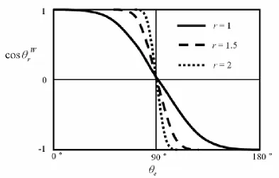
In Wenzel’s approach the liquid fills the grooves on the rough surface (Figure 2.5a). According to Wenzel, the liquid contact angle at a rough surface can be described as: 39

e W

r r θ

θ cos

(23)

(a) (b)

Figure 2.5. A liquid drop (a) wetting the grooves of a rough surface (Wenzel model) and (b) sitting at the top of a rough surface (Cassie-Baxter model).

(24)

Figure 2.6. Cosine curves of apparent contact angles depending on roughness, r.

The Cassie and Baxter model is an extended form of the Wenzel model to include porous surfaces. In this model a liquid sits on a composite surface made of a solid and air. Therefore, the liquid does not fill the grooves of a rough solid. In their paper published in 1944, Cassie and Baxter suggested that:40

2 1cos

cosθ_rCB = f θ_e− f (2.20)

where f1 is the surface area of the liquid in contact with the solid divided by the projected

area, and f2 is the surface area of the liquid in contact with air trapped in the pores of the

rough surface divided by the projected area. According to Cassie and Baxter:

area Projected

liquid th contact wi in

Area 1 =

(25)

area Projected

air th contact wi in

Area 2 =

f (2.22)

When there is no trapped air, f1 is identical to the value of r in the Wenzel model.

Recognizing this, equation (2.25) has recently been rewritten as follows:

f r

f1 = f (2.23)

f

f₂ =1− (2.24)

1 cos

cos CB =r_f f _e + f −

r θ

θ (2.25)

where f is the fraction of the projected area of the solid surface in contact with the liquid and rf is defined by analogy with the Wenzel model.41 It is important to note that rf in equation (2.25) is not the roughness ratio of the total surface, but only of that in contact with the liquid. In this form of the Cassie-Baxter equation, the contributions of surface roughness and of trapped air are much clearer than in the other forms of the equation.

Recently, many authors used another approach for the Cassie-Baxter equation to describe contact angles of droplets on heterogeneous rough surfaces that have composite interfaces.42 In the modified Cassie and Baxter model the liquid forms a composite surface made of solid, liquid and air; and the liquid does not fill the grooves on the rough surface (Figure 2.5b).43 When the top of a rough surface is completely flat, the following equation describes the apparent contact angle on a rough surface:44

2 2 1

1cos cos

cosθ CB =Φ θ +Φ θ

r (2.26)

(26)

of the surface has a unit surface area fraction Φ1 with a contact angle θ1 and an area fraction

Φ2 with a contact angle θ2. When this rough surface consists of only two materials Φ2 = 1 –

Φ1. If the liquid does not completely wet the surface, Φ2 represents the trapped air with θ2

=180º. Equation (2.20) can be modified as:45 1 ) 1 (cos 1

cos

cos CB=Φ_S _e+Φ_S − =Φ_S _e+ −

r θ θ

θ (2.27)

2 2

) (a b

a

S _Σ ₊ Σ =

Φ (2.28)

where ΦS is the ratio of the rough surface area in contact with a liquid drop to the total surface covered by a liquid drop, a is the width of a prominence of a rough surface and b is the distance between prominences. Smaller ΦS increases θrCB and makes the surface more hydrophobic (Figure 2.7).

(27)

For an apparent contact angle of water on TeflonTM to be greater than 150º (superhydrophobic), the fraction of the surface in contact with water must be less than 26%.46

2.2.3. Modeling of artificial lotus fabric

(28)

Figure 2.8. Upper-sectional view of roughness pattern.

The pillar cross-sectional area is a2_{, the distance between two pillars is}_d_{, and the}

height of pillar is h. In an analysis of the superhydrophobic effect, Patankar has provided two equations to describe the surface based on the Wenzel (equation (2.19)) and the Cassie-Baxter (equation (2.21)) models:52 53

e W r _a h d a a _θ

θ 4 1 cos

cos 2 ⎟ ⎟ ⎠ ⎞ ⎜ ⎜ ⎝ ⎛ + ⎟ ⎠ ⎞ ⎜ ⎝ ⎛ +

= (2.29)

1 ) 1 (cos cos 2 − + ⎟ ⎠ ⎞ ⎜ ⎝ ⎛ + = _e CB

r _a _d

a _θ

θ (2.30)

(29)

In recent literature, the Cassie-Baxter model is often described using the apparent contact angle on a rough surface by equation (2.27).54 55_{Note that the form of the}

(30)

2.3. Contact angle hysteresis

(31)

volume of the drop increases.60 In addition, Hennig et al. demonstrated that the contact angle hysteresis of a smooth film depends on the contact time with water.61

Figure 2.9. Self-cleaning effect by superhydrophobicity.

Since surface debris sticks to the drop surface and is removed when the drop rolls off, the superhydrophobic surface has self-cleaning effect. The difference between the advancing angle and the receding angle is the contact angle hysteresis defined as ΔθH. The contact angle hysteresis is very important in understanding the drop motion on a surface.

2.3.1. Sliding angle

(32)

R k

mgsinα = 2π (2.31)

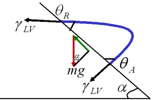
where α is the sliding angle, R is the radius of the contact circle, m is the mass of the droplet, g is the gravitational acceleration, and k is a proportionality constant. Roura and Fort demonstrated the work due to the external forces on a drop in Figure 2.10.63

Figure 2.10. Water drops on a tilted surface.

Figure 2.10 shows that the advancing contact angle is always greater than the receding contact angle on a tilted surface. This condition was described by Furmidge as:

) cos (cos

2

sin R _LV _A _R

mg α ≈− γ θ − θ (2.32)

When the surface is tilted, the tilt angle increases until the drop begins to move and equation (2.32) can be expressed in terms of working energy if the drop slides down as shown in Figure 2.10.

As mentioned before, it is assumed that the receding contact angle and the advancing contact angle seem to be close to their minimum and maximum values, respectively when the drop slides down (α = αc):

) cos

(cos 2

sin R

(33)

Equation (2.33) shows an energy balance when the solid surface is progressively inclined and the drop begins to slide at αc. In this situation, gravity can supply the necessary energy to develop the back wetted surface, and thereby the energy used to create a unit area of this surface is – 2RγLV (cosθA(max) – cosθR(min)). Although the contact angle changes continuously

along the contact line, equation (2.33) can be approximately calculated. The constant k in equation (2.31) is related to contact angle hysteresis, and the interfacial surface tension between water and vapor.

When the surface is superhydrophobic and the droplet is close to spherical:

ρ π₍ _'₎3 3 4

R

m= (2.34)

where ρ is the density of water and R’ is the radius of droplet. By multiplying gsinαc to both sides we can describe the relationship between the radius of the contact circle and the radius of droplet sliding on a smooth surface as:

c

c R g

mg α π( ') ρ sinα

3 4

sin ₌ 3 _(2.35)

Substituting equation (2.35) into equation (2.33), we obtain: )

cos (cos

'

sinαc =k θA(max) − θR(min) (2.36)

(34)

2.3.2. Contact angle hysteresis

(35)

(a)

(b)

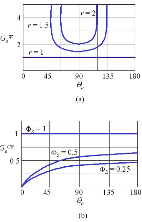
Figure 2.11. Gain factors on rough surfaces for (a) r = 1, 1.5 and 2 (Wenzel model) and (b) ΦS = 0.25, 0.5 and 1 (Cassie-Baxter model).

The Wenzel equation gives a change in the Wenzel contact angle, ΔθHW, caused by a change in the contact angle on the smooth surface, ΔθH, as:

H W e H W r

e W

H r _θ θ G θ

θ

θ _⎟⎟Δ = Δ

⎠ ⎞ ⎜⎜

⎝ ⎛ = Δ

sin sin

(2.37)

where GeW is the Wenzel gain factor, and is . The gain factor is very useful, for it separates the idea of the equilibrium contact angle increase occurring by surface

(36)

topography from the observed contact angle. Using the Wenzel equation we can obtain the Wenzel gain factor as follows:

e W

r r θ

θ 2 2

2 _cos

cos =

e W

r r θ

θ 2 2

2 ₁ _cos

cos

1− = −

e W

r r θ

θ ₁ 2_cos2

sin = −

e e W r e W e r r r G θ θ θ θ 2 2_cos 1 sin sin sin − =

= (2.38)

When a contact angle θe is close to 90° the Wenzel gain factor is approximately unity. Since the effect of roughness is proportional to the radian contact angle changes, the Wenzel gain factor rapidly increases as the roughness factor increases.

Likewise, Cassie-Baxter equation gives a change in the Cassie-Baxter contact angle, ΔθHCB, caused by a change in the contact angle on the smooth surface, ΔθH, as:

H CB e H CB r e S CB

H _θ θ G θ

θ θ _⎟⎟Δ = Δ ⎠ ⎞ ⎜⎜ ⎝ ⎛ Φ = Δ sin sin (2.39)

In a similar manner as above, a Cassie-Baxter gain factor, GeCB, can be obtained by the Cassie-Baxter equation as follows:

[

]

2

2 _(cos ₁₎ ₁

cos CB = Φ_S _e + −

r θ

θ

[

]

2

2 ₁ _(cos ₁₎ ₁

cos

1− CB = − Φ_S _e + −

r θ

θ

[

]

2

1 ) 1 (cos 1

sin CB = − Φ_S _e + −

r θ

(37)

[

]

2 1 ) 1 (cos 1 sin sin sin − + Φ − Φ = Φ = e S e S CB r e S CB e G θ θ θ θ (2.40)

Since ΦS ≤ 1, GeCB ≤ 1. The θe used in equations (2.37) and (2.39) can be either the advancing or receding contact angles. Thus, the contact angle hystereses are:

H W e W

H G θ

θ = Δ Δ H CB e CB

H G θ

θ = Δ

Δ

(38)

3. PRODUCT AND TECHNOLOGY REVIEW

3.1. Research review

Over the last 15 years, many studies of superhydrophobicity and contact angle hysteresis have been performed. Recently, Zhu et al. developed a superhydrophobic surface by electrospinning using a hydrophilic material, poly(hydroxybutyrate-co-hydroxyvalerate) (PHBV). 65 Gao and McCarthy made artificial super-hydrophobic surfaces with conventional polyester and microfiber polyester fabrics rendered hydrophobic by using a simple patented water-repellent silicone coating procedure. 66 Lee and Michielsen developed superhydrophobic surfaces via the flocking process and achieved contact angles as high as 178°.67 Jopp et al. researched the wetting behavior of water droplets on periodically structured hydrophobic surfaces and the effect of structure geometry.68 Liu et al. studied the creation of stable superhydrophobic surfaces using vertically aligned carbon nanotubes.69 Nakajima et al. prepared superhydrophobic thin films with TiO2 photocatalyst

(39)

can be applied to microfluidic devices by preparing a stable superhydrophobic surface via aligned carbon nanotubes (CNTs) coated with a zinc oxide (ZnO) thin film.73 Shang et al.

prepared optically transparent superhydrophobic silica-based films on glass substrates by making a nanoscale rough surface using nanoclusters and nanoparticles.74 Shi et al.

(40)

3.2. Patent review

(41)

Buchsel et al. invented method of producing self-cleaning and non-adhesive paper or paper-like material.81 The patent describes that a micro-structured paper or paper-like material having a self-cleaning and/or non-adhesive effect is hydrophobic across the entire cross-section of the material. The surface of materials is micro-structured in such a way that the surface is provided roughness whereby the distance between the elevations ranges from 0.04 to 100 μm and the height of the elevations ranges from 0.04 to 100 μm. This material contains particles having the size of 0.04 to 50 μm that are bound to the paper or paper-like material through binding. The paper or paper-like material becomes hydrophobic across the entire cross section of the material and has self-cleaning effect.

(42)

with a catalytically active second layer. Then, the substrate has microstructured crystal coating for self-cleaning effect.

(43)

equipment. At least one surface from this molding has self-cleaning effect and the surface has particles with a fissured structure.

Wang also invented the Lotus leaf-like self-cleaning surface structure.85 A self-cleaning surface structure formed of a coating mixture covered on the surface of a product. The coating mixture contains a polymeric resin having low surface tension and a nano sized metal oxide compound (i.e., nanosize TiO2). The polymeric resin serves as a medium to

(44)

3.3. Applications in industry

BASF researchers developed the MincorTM coating system in which they applied the Lotus effect observed in nature.86 The effect of their laboratory product is based on a combination of nanoparticles and hydrophobic polymers.87 MincorTM is applicable not only to textiles but also to mineral plasters, concrete, brick facing, and even to wood (Figure 3.1).

88

(a) (b)

Figure 3.1. A water droplet (a) on a wood surface coated with MincorTM and (b) containing dirt on a superhydrophobic surface. (Source: BASF Photos).

Thus, MincorTM can be used as an adhesive to improve hydrophobic effect in the area of construction. The extreme water repellency of this spray minimizes the adhesion among water drops and material surfaces; rain water rolls off immediately; and the surface is always dry and clean.

(45)

(46)

4. EXPERIMENTAL

4.1. Materials

Nylon 6,6 film (Mn:12 kD), nylon 6,6 multifilament plain woven fabric (weight:

100 g/m2), nylon 6,6 monofilament plain woven fabric (weight: 100 g/m2), nylon 6,6 calendered monofilament modified twill woven fabric (weight: 100 g/m2), and flock fabrics were used as smooth or rough surfaces. To prepare flock fabrics, various nylon 6,6 rod-shaped short fibers (flock, Cellusuede), polyester fabric (93 g/m2), acrylic adhesive (C. L. Hauthaway & Sons Co.), and an electrostatic flock applicator (CP-70, Cellusuede Products. Inc.) were used. Poly(acrylic acid) (PAA, Mw: 450 kD, Aldrich),

4-(4,6-dimethoxy-1,3,5-triazin-2yl)-4-methylmorpholinium chloride (DMTMM, Fluka), sodium thiocyanate (NaSCN, Fisher), methanol (CH3OH, Aldrich), 1H, 1H-perfluorooctylamine (C8H4F15N,

(47)

4.2. Preparation of rough nylon surfaces

(48)

(49)

4.3. Surface modification of nylon 6,6 4.3.1. Grafting of PAA on nylon 6,6 surface

Since nylon 6,6 has few reactive groups on the surface and since we wish to chemically graft an alkyl or fluoroalkyl material to the surface, poly(acrylic acid), PAA, was first grafted to the nylon surface to increase the number of reactive sites following the procedure developed by Thompson.92 1 g PAA was dissolved in 250 mL distilled water at 20 ºC. Then 0.5 g nylon film (10 x 10 cm2) and 1g of each nylon woven fabric (10 x 10 cm2) were immersed in the PAA solution for 24 hours, rinsed in distilled water with stirring for 8 hours (repeated three times with fresh water), wiped with Kimwipes® and air dried.

0.1 g DMTMM was dissolved in distilled water with vigorous stirring at 20 ºC. PAA adsorbed nylon materials were immersed in the DMTMM solution to graft PAA to the nylon surfaces. The reaction was allowed to proceed for 2 hours. PAA-grafted nylon materials were rinsed in distilled water for 8 hours (repeated three times with fresh solvent), wiped with Kimwipes®, and air dried.

(50)

Scheme 4.1. Graft of PAA on nylon 6,6.

4.3.2. Grafting of fluoroamine on PAA-grafted nylon 6,6 surface

0.05 g 1H, 1H-perfluorooctylamine was dissolved in 10 mL methanol at 20ºC. Then 0.15 g PAA-grafted nylon film (5 x 6 cm2) and 0.3 g of each PAA grafted nylon woven fabric (5 x 6 cm2) were immersed in the 1H, 1H-perfluorooctylamine solution for 24 hours with stirring to allow adsorption of 1H, 1H-perfluorooctylamine.

0.03 g DMTMM was dissolved in methanol with vigorous stirring at 20ºC. 1H, 1H-perfluorooctylamine adsorbed PAA-grafted nylon materials were immersed in the DMTMM solution to graft 1H, 1H-perfluorooctylamine to the PAA on nylon 6,6 surfaces. The reaction proceeded for 2 hours. The 1H, 1H-perfluorooctylamine-grafted PAA-grafted nylon materials were rinsed in methanol for 8 hours (repeated twice with fresh solvent), rinsed in distilled water for 8 hours (repeated twice with fresh solvent), wiped with

CO2H

NH2

CO2H

O

OH

PAA

+

DMTMM

Nylon

CO2H

NH3+

CO2H

O -_O PAA-absorbed-Nylon N N N OCH3 N+ O H3C

OCH3

Cl

-CO2H

N H

CO2H

O

(51)

Kimwipes®, and air dried. Scheme 4.2 shows the grafting procedure for 1H, 1H-perfluorooctylamine on PAA-grafted nylon 6,6.

Scheme 4.2. Graft of 1H, 1H-perfluorooctylamine on PAA-grafted nylon 6,6.

4.3.3. Grafting of octadecylamine on PAA-grafted nylon 6,6 surface

0.03 g octadecylamine was dissolved in 10 mL methanol at 20ºC. Then 0.15 g PAA-grafted nylon film and 0.3 g of each PAA-PAA-grafted nylon woven fabric were immersed in the octadecylamine solution for 24 hours with stirring to allow adsorption of octadecylamine.

0.03 g DMTMM was dissolved in methanol with vigorous stirring at 20 ºC. Octadecylamine adsorbed PAA-grafted nylon materials were immersed in the DMTMM solution to the graft octadecylamine to the PAA on nylon 6,6 surfaces. The reaction proceeded for 2 hours. The octadecylamine-grafted PAA-grafted nylon materials were rinsed in methanol for 8 hours (repeated twice with fresh solvent), rinsed in distilled water

DMTMM

CO2H

N H

CO2H

O

PAA-grafted-Nylon

CO2H

N H

O

Perfluorooctylamine-grafted-PAA-grafted-Nylon

CONHCH2(CF2)6CF3

(52)

for 8 hours (repeated twice with fresh solvent), wiped with Kimwipes®, and air dried. Scheme 4.3 shows the grafting procedure for octadecylamine on PAA-grafted nylon 6,6.

Scheme 4.3. Graft of octadecylamine on PAA-grafted nylon 6,6.

DMTMM

CO2H

N H

CO2H

O

PAA-grafted-Nylon

CO2H

NH2

O

Perfluorooctylamine-grafted-PAA-grafted-Nylon

CONHCH2(CH2)16CH3

(53)

4.4. Characterization

4.4.1. Scanning electron microscopy

The rough surface nylon composite was examined with a scanning electron microscope (SEM), Hitachi S-3200N, operated at 5 kV and 10 kV and magnifications from 25x to 2000x magnification. Image J 1.34s (National Institute of Health) was used for image analysis of SEM pictures. On a rough surface, the diameters and distances among adjacent protuberances or grooves were measured using this program.

4.4.2. Contact angle measurements

(54)

5. RESULTS AND DISCUSSIONS

To form a superhydrophobic surface, the surface must have a low surface tension and be rough. We used a two stage procedure to create a superhydrophobic fabric. First, we modified nylon film to generate a low surface tension surface. Then we made a rough nylon surface via the flocking process and modified the nylon flock fibers to give them a low surface tension using the same procedure as for the nylon film. Similar studies were performed on woven fabrics and calendered woven fabrics. A water droplet easily rolled off of the superhydrophobic surfaces at a very low incline angle.

5.1. Chemical surface modification of nylon 6,6

The wetting behavior of a solid surface is controlled by both the surface tension and the geometric structure of the surface. To form a superhydrophobic surface, the surface has to have a low surface tension and an appropriate roughness. First, we verified that the chemical procedure described in the experimental section resulted in a low surface energy on smooth nylon 6,6 films.

(55)

predicted value as shown in Table 5.1. Figure 5.1 presents a water droplet sitting on a smooth nylon film; the equilibrium water contact angle on this surface is 70º.

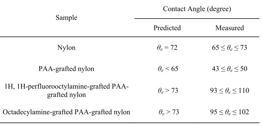
Table 5.1. Comparison of predicted and measured water contact angles on smooth surfaces Contact Angle (degree)

Sample

Predicted Measured

Nylon θe = 72 65 ≤ θe ≤ 73

PAA-grafted nylon θe < 65 43 ≤ θe ≤ 50 1H, 1H-perfluorooctylamine-grafted

PAA-grafted nylon θe > 73 93 ≤ θe ≤ 110 Octadecylamine-grafted PAA-grafted nylon θe > 73 95 ≤ θe ≤ 102

(56)

(57)

Figure 5.2. A water droplet on a PAA-grafted nylon surface. The water contact angle on this surface is 43º.

(58)

Figure 5.3. A water droplet on a 1H, 1H-perfluorooctylamine-grafted PAA-grafted nylon surface. The water contact angle on this surface is 100º.

(59)

5.2. Preparation of superhydrophilic rough surfaces 5.2.1. Superhydrophilic flock surfaces

The next step in the process of making a superhydrophilic material is to generate an appropriate rough surface. The predominant approach to model a superhydrophilic rough surface is the Wenzel model. According to the model, a surface of a composite material can be superhydrophilic when the material consists of a rough surface having appropriate roughness, r, as shown in equations (2.19). In this study, rod-shaped nylon flock fibers were attached on a polyester substrate. The protruding flock fibers can be thought of as pillars sticking up from the fabric surface as depicted in Figure 5.4.

Figure 5.4. Side and upper views of roughness pattern.

(60)

(

2

)

1 2 2 + + = d R Rh

r π (5.1)

where R and h are the radius and height of a flock fiber, respectively; and d is the distance between two adjacent fibers. Reformulating the Wenzel equation gives:

(

)

e

W r d R Rh _θ π

θ 1 cos

2 2

cos ₂ _⎟⎟

⎠ ⎞ ⎜⎜ ⎝ ⎛ + +

= (5.2)

Four kinds of rough surfaces having different dimensions were fabricated. Table 5.2 describes the geometric parameters of the nylon fibers used to generate the rough surfaces. Each surface is identified as nylon flock, NF, and the height to radius ratio. For example, NF70 is made with nylon flock fibers with a height to radius ratio of 70.

Table 5.2. Dimensions of pillar shaped nylon flock fibers

dtex* Radius** (μm)

Height

(μm) Height / Radius

NF50 3.3 10 500 50

NF70 1.7 7 500 70

NF100 3.3 10 1000 100

NF140 1.7 7 1000 140

* Linear density: 1 dtex = 1g / 10,000m

** Calculated from linear density of each fiber and density of nylon 6,6 (1.14 g/cm3) Sample

(61)

Table 5.3 shows the measured interfiber distances between adjacent fibers determined at 20 different locations. The Wenzel roughness, r, on each sample was calculated by using equation (5.2).

Table 5.3. Measured distances between two adjacent flock fibers and roughness, r

Sample Measured distance*

(μm) Roughness, r

NF50 5 ≤d≤ 120 2.6 ≤r≤ 51.3

NF70 10 ≤d≤ 120 2.2 ≤r≤ 39.2

NF100 25 ≤d≤ 76 7.8 ≤r≤ 32.0

NF140 10 ≤d≤ 78 6.2 ≤r≤ 77.4 * Measured at twenty random spots

(62)

Figure 5.5. SEM views from above and from side of NF140 (50x).

(63)

Table 5.4. Comparison of predicted and measured apparent contact angles of superhydrophilic flock surfaces

Apparent contact angle (degree)

Nylon PAA-grafted nylon

Sample

Predicted Measured Predicted Measured

NF50 θr = 0 θr ≈ 0 θr = 0 θr ≈ 0

NF70 θr = 0 θr ≈ 0 θr = 0 θr ≈ 0

NF100 θr = 0 θr ≈ 0 θr = 0 θr ≈ 0

NF140 θr = 0 θr ≈ 0 θr = 0 θr ≈ 0

Figure 5.6. A water droplet on a nylon NF50 surface. The apparent water contact angle on this surface is close to 0º.

(64)

structure and the water contact angles of PAA-grafted rough surfaces are 0°. Again, excellent agreement is found between the predicted values of the apparent contact angle and the measured values when the contact angle follows the Wenzel model and θe is less than 90°. Figure 5.7 shows a water droplet completed immersed into the fabric structure of PAA-grafted nylon NF50. The apparent water contact angle on this surface is 0º.

Figure 5.7. A water droplet on a PAA-grafted nylon NF50 surface. The water contact angle on this surface is 0º.

5.2.2. Superhydrophilic plain woven surfaces

(65)

monofilament yarns. The surface area of a single round monofilament yarn in the unit fabric can be calculated based on Figure 5.8.

(a) (b)

Figure 5.8. The cross section views of a plain woven fabric: at the warp yarn direction (a) and at the weft yarn direction (b).

For this rough surface, r is defined using flux integral. As shown in Figure 5.8, the distance from the center of a weft yarn to the center of an adjacent weft yarn is 4R; in the same manner, the distance from the center of a warp yarn to the center of an adjacent warp yarn is 4R; and the distance from the center of a weft yarn to the center of an adjacent warp yarn is 2R. Hence, according to Pythagorean theorem, the vector from the center of one weft yarn to the center of an adjacent weft yarn makes a 30° angle to the plane of the fabric. Using flux integral, the area of one yarn in the unit fabric is calculated as:

vk R uj v R R ui v R R v u

r( , )=(2 + cos )cos +(2 + cos )sin + cos

uj v R R ui v R R

r_u =−(2 + cos )sin +(2 + cos )cos

vk R uj v R ui v R

r_v =− sin cos − sin sin + cos

vk v R R R vj u v R R R vi u v R R R r

(66)

) cos 2

( R R v R

r

r_u× _v = +

3 ) cos 2 ( 2 0 2 0

∫ ∫

+ = π π dudv v R R R A_yarn_in_unit_area

area unit in yarn warp area unit in yarn weft area unit in

yarn A A

R

A = = =

3 8_π2 2

(5.3)

where R is the radius of yarn; A is the area; i, j and k are the vectors to x, y, and z axis direction, respectively; u and v are the notations for the variables of integration. Then, we determine the true fabric surface area as follows:

area unit in yarn warp area unit in yarn weft real

fabric A A

A = + (5.4)

where Arealfabric is the intrinsic area of the unit fabric determined by the area of yarn surfaces. We have two yarns in the unit area. Substituting equation (5.3) into equation (5.4) gives:

2 64 . 52 R Areal

fabric = (5.5)

The apparent surface area is just equal to the area of a plane tangent to the top surface. 2

12 3 2 3

2 R R R

Aapparent

fabric = × = (5.6)

where Aapparentfabric is the apparent area of the unit fabric shown in Figure 5.8. Finally, the roughness, r, is just the ratio of these areas:

39 . 4 12 64 . 52 2 2 = = = R R A A r _apparent fabric real fabric (5.7)

(67)

yarn in the unit cell is 8πR2. There are two yarns in a unit cell, one warp and one weft. Thus, the true surface area for the entire thickness of a monofilament plain woven fabric is 16πR2

as shown in equation (5.3). The apparent surface area is just equal to the area of a plane tangent to the top surface as shown in equation (5.6). Finally, the roughness, r, is just the ratio of these areas:

19 . 4 3 4

= ≈ = _apparent π

fabric real fabric

A A

r (5.8)

(68)

Table 5.5. Comparison of predicted and measured apparent contact angles of superhydrophilic woven surfaces

Apparent contact angle (degree)

Nylon PAA-grafted nylon

Sample

Predicted Measured Predicted Measured Monofilament

woven fabric θr = 0 θr ≈ 0 θr = 0 θr ≈ 0

Multifilament

woven fabric θr = 0 θr ≈ 0 θr = 0 θr ≈ 0

Next, we look at a plain woven fabric made with multifilament yarns. Clearly, a multifilament yarn will have even higher values of r, since the space between the fibers will increase the real surface area while the apparent surface area remains the same. In this case, equation (5.3) becomes:

f multi

real

fabric A R NR

A = ≈52.64 × (5.9)

where N is the number of filament fibers, R is the radius of the yarn, and Rf is the radius of the filament fibers. Substituting equation (5.9) into equation (5.7) yields:

R NR R NR A A

r _apparent f f

fabric real fabric 39 . 4 3 4 = ≈

= π (5.10)

(69)

Figure 5.9. SEM micrographs of a multifilament plain woven fabric.

(70)

Figure 5.10. A water droplet absorbed into plain woven structure made of nylon multifilament fibers. The water contact angle on this surface is 0º.

5.2.3. Modeling of other superhydrophilic woven surfaces

(71)

Figure 5.11. The cross section views of a 2/1 twill woven fabric.

As shown in Figure 5.8, the distance from the center of a weft (or warp) yarn to the center of an adjacent weft (or warp) yarn is 4R, and the distance from the center of a weft (warp) yarn to the center of an adjacent warp (weft) yarn is 2R. Hence, the vector from the center of one weft yarn to the center of an adjacent weft yarn, or the vector from the center of one warp yarn to the center of an adjacent warp yarn, makes a 30° angle to the plane of the fabric, as the plain woven fabric does. Therefore, the area of one yarn in the unit fabric is calculated as:

2 2 0 2 0 3 ) cos 2 ( R dudv v R R R

A_yarn_in_unit_area π

π π + + =

∫ ∫

yarn R A A

A = 2 + ₎ 2 = =

3 8

( π π (5.11)

Then, we determine the true fabric surface area as follows.

2 2 ) 3 8 ( 2 R A A

Areal _weft_yarn_in_unit_area _warp_yarn_in_unit_area fabric

π

π +

= +

(72)

where Arealfabric is the intrinsic area of the unit fabric determined by the area of yarn surfaces. We have four yarns in the unit area. Therefore, the real fabric area is:

2 2 ₂₁₈_.₈₂ ) 2 64 . 52 (

4 R R

Areal

fabric = + π = (5.13)

The apparent surface area is just equal to the area of a plane tangent to the top surface. 2 85 . 29 ) 1 3 ( 2 ) 1 3 (

2R R R

Aapparent

fabric = + × + = (5.14)

where Aapparentfabric is the apparent area of the unit fabric shown in Figure 5.11. Finally, the roughness, r, is just the ratio of these areas:

33 . 7 85 . 29 82 . 218 2 2 = = = R R A A r _apparent fabric real

fabric _(5.15)

Since r = 7.33, and the measured contact angles 65º ≤ θe ≤ 73º on the flat nylon film and 43º ≤ θe ≤ 50º on the flat PAA-grafted nylon film into equation (2.19), θrW = 0º for both fabrics regardless of PAA-grafting. Indeed, the predicted values were in good agreement with the measured angles although we reformed the 2/1 twill woven surface, which was calendered by heat, was used for this experiments (Table 5.5).

In the same manner, the Wenzel roughness, r, of 3/1 twill fabrics can be obtained. Figure 5.12 shows a cross sectional view of a model of a 3/1 twill woven fabric made from monofilament yarns. The surface area of a single round monofilament yarn in the unit fabric can be calculated based on Figure 5.12.

(73)

Figure 5.12. The cross section views of a 3/1 twill woven fabric.

The area of one yarn in the unit fabric is calculated as:

2 2 0 2 0 ₂ 3 ) cos 2 ( R dudv v R R R

A_yarn_in_unit_area π

π π + + =

∫ ∫

yarn R A A

A = 2 +₂ ₎ 2 = =

3 8

( π π (5.16)

Then, we determine the true fabric surface area as follows:

2 2 ) 3 2 8 ( 2 R A A

Areal _weft_yarn_in_unit_area _warp_yarn_in_unit_area fabric

π

π +

= +

= (5.17)

where Arealfabric is the intrinsic area of the unit fabric determined by the area of yarn surfaces. We have six yarns in the unit area. Therefore, the real fabric area is:

2 2 ₃₅₃_.₅₉ ) 2 64 . 52 (

6 R R

Areal

fabric = + π = (5.18)

The apparent surface area is just equal to the area of a plane tangent to the top surface. 2 71 . 55 ) 2 3 ( 2 ) 2 3 (

2R R R

Aapparent

fabric = + × + = (5.19)

(74)

35 . 6 71

. 55

59 . 353

2 2

= =

=

R R A

A r _apparent

fabric real fabric

(5.20)

(75)

5.3. Preparation of superhydrophobic rough surfaces 5.3.1. Superhydrophobic flock surfaces

The next step in the process of making a superhydrophobic material is to take the rough surfaces and make them hydrophobic. The predominant approach of modeling a superhydrophobic rough surface is the Cassie-Baxter model. According to this model, a surface of a composite material can be superhydrophobic when the material consists of a rough surface having the appropriate area fraction of the surface in contact with water, ФS, as shown in equations (2.27). In this study, rod-shaped nylon flock fibers were attached on a polyester substrate. The protruding flock fibers can be thought of as pillars sticking up from the fabric surface as depicted in Figure 5.4.

For this rough surface, ФS is defined as:

(

)

2

2R d R

S = ₊

Φ π (5.21)

where R and h are the radius and height of a flock fiber, respectively; and d is the distance between two adjacent fibers. Reformulating the Cassie-Baxter equations gives:

(

2

)

(

cos 1

)

1

cos ₂

2

− + +

= _e

CB r

d R

R _θ

π

θ (5.22)

(76)

tension material such as poly(tetrafluoroethylene, PTFE) (θe ≈ 119°). The graph shows that this rough surface becomes superhydrophobic when ΦS ≤ 26%.

Figure 5.13. Plots of apparent water contact angles on a fluoroamine covered rough surface in Cassie-Baxter model; Crosshatched area indicates the superhydrophobic region.

(77)

Table 5.6. Measured distances between two adjacent flock fibers and top area fraction, ΦS

Sample Measured distance*

(μm) Top area fraction, ΦS NF50 5 ≤d≤ 120 0.02 ≤ΦS ≤ 0.50

NF70 10 ≤d≤ 120 0.01 ≤ΦS ≤ 0.26

NF100 25 ≤d≤ 76 0.03 ≤ΦS ≤ 0.16

NF140 10 ≤d≤ 78 0.02 ≤ΦS ≤ 0.26 * Measured at twenty random spots

(78)

Table 5.7. Comparison of predicted and measured apparent contact angles of hydrophobic and superhydrophobic flock surfaces

Apparent contact angle (degree) Sample

Predicted Measured

NF50 122 ≤ θr ≤ 171 132 ≤ θr ≤ 140

NF70 139 ≤ θr ≤ 173 168 ≤ θr ≤ 175

NF100 148 ≤ θr ≤ 169 170≤ θr ≤ 178

NF140 140 ≤ θr ≤ 171 170 ≤ θr ≤ 178

(79)

rough surface, which indicates that the water droplet is sitting on the top of flock fibers and follows the Cassie-Baxter model.

Figure 5.14. A water droplet on a superhydrophobic surface of NF70. Lights under the droplet show that water is sitting on the top of the flock fibers.

(80)

5.3.2. Superhydrophobic woven surfaces

To make a superhydrophobic surface, we first need to make the surface hydrophobic and create the appropriate roughness. According to Cassie and Baxter, and Marmur, and as is evident from equations (2.25) and (2.30), the Wenzel model is a special case of the Cassie-Baxter equation where f = 1 and rf = r (equation 2.30). For a material with a smooth surface water contact angle of 93° (as above), the Wenzel surface roughness,

r, must be greater than 16.5 for the apparent contact angle to exceed 150°. However, according to Marmur, the minimization of the free energy requires that, for a hydrophobic surface with f = 1, θe = 180°. Since the only material known with θe = 180° is air or vacuum,

f cannot be equal to one. In other words, the Wenzel model is invalid for hydrophobic surfaces. In order to develop superhydrophobic surfaces, we need to use a different approach, namely the Cassie-Baxter model.

(81)

simple differentials we obtain d(rff) / drf = (cosα)-1 and d(rff)2 / drf2 > 0 in both (a) and (b). According to Marmur, under these conditions, there is a minimum surface free energy on each surface such that α = π – θe. Substituting for f and rf for case (b) into equation (2.30) results in:

1 sin cos

cos ⎟ −

⎠ ⎞ ⎜ ⎝ ⎛ + + ⎟ ⎠ ⎞ ⎜ ⎝ ⎛ + − = α α α θ d R R d R R CB

r (5.23)

(a) (b)

Figure 5.15. A liquid drop sitting on (a) cylinders packed tightly, and (b) cylinders separated by a distance, 2d. α = π – θe.

On substituting π – θe for α, we obtain:

(

)

cos sin 1

cos ⎟ −

⎠ ⎞ ⎜ ⎝ ⎛ + + − ⎟ ⎠ ⎞ ⎜ ⎝ ⎛ +

= _e _e _e

CB r d R R d R

R _π _θ _θ _θ

θ (5.24)

For θe > 90°, θrCB_{increases with increasing}_d_{. For example, when θe = 120° and}_d_{= 0, the} fibers are closely packed and θrCB = 131°; for d = R, θrCB = 146°; and for d = 2R, θrCB = 152°.

(82)

(83)

Table 5.8. Comparison of predicted and measured apparent contact angles of hydrophobic and superhydrophobic woven surfaces

Apparent contact angle (degree) 1H,

1H-perfluorooctylamine-grafted nylon woven fabric

Octadecylamine-grafted nylon woven fabric Sample

Predicted Measured Predicted Measured Monofilament

woven fabric 118 ≤ θr ≤ 134 130 ≤ θr ≤ 138 120 ≤ θr ≤ 127 125 ≤ θr ≤ 134

Multifilament

yarn 123 ≤ θr ≤ 138 N/M* 125 ≤ θr ≤ 131 N/M Multifilament

woven fabric 146 ≤ θr ≤ 158 160≤ θr ≤ 168 147 ≤ θr ≤ 152 155≤ θr ≤ 168 Calendered

woven fabric 112 ≤ θr ≤ 127 109 ≤ θr ≤ 113 114 ≤ θr ≤ 120 107 ≤ θr ≤ 110 * Not measured

In the second case, we again extend the analysis to a multifilament fabric. We begin by determining the apparent contact angle of the liquid with the multifilament yarns. From Figure 5.9, it is seen that the fiber spacing is approximately equal to the fiber diameter, i.e.

(84)

) 1 3 ( − =R

d such that 2(R + d) = 2 3R as before. We obtain 146° ≤ θrCB ≤ 158° for the 1H, 1H-perfluorooctylamine-grafted fabric, and 147° ≤ θrCB≤ 152° for the octadecylamine-grafted fabric. As seen in Table 5.8, the measured values are slightly larger than our predicted values. This is probably due to the real value of d being larger than the values chosen in this analysis. For example, the surface of the fabric shown in Figure 5.9 clearly has loose fibers on the surface that are not entrained in the yarn. These surface fibers are separated from the remainder of the fibers by distances d > R. As shown earlier, larger values of d result in larger values of θrCB. Thus the measured values of θrCB are greater than predicted values. Figure 5.16 shows a water droplet sitting on this surface; the apparent water contact angle on this surface is 168º.

(85)

Others have reported the Cassie-Baxter model using equation (2.21). This form of the Cassie-Baxter equation is valid only when a surface is perfectly smooth (i.e. ΦS = r = 1) or when the top of a rough surface is flat. Comparing equation (2.21) to equations (2.25) and (2.30) shows that equation (2.25) is only correct when f1 + f2 = 1. However, f1 + f2 > 1

on general rough surfaces. For example, in the multifilament yarns of Figure 5.9, )

1 3 ( − =R

d , θe≈100° giving f1 = 0.81 and f2 = 0.43 since:

(

e

)

d R

R

f π −θ

+ =

1 (5.25)

e

d R

R

f₂ 1 sinθ

+ −

= (5.26)

Thus, in this case, f1 + f2= 1.24. This is clearly not equal to one and equation (2.21) cannot be applied in this case. Rather, the original Cassie-Baxter equation is preferred.

An additional surface structure was analyzed using flattened fibers, which resulted in a smoother fabric. Figure 5.17 shows another woven fabric made of monofilament yarns that have been calendered. In this case, the fraction of the surface in contact with water, f1,

must be larger than that of round fibers since water will contact more of the surface of these flattened yarns. f1 + f2 is also greater than one on this rough surface. Since it is difficult to

measure f1 and f2 of calendered fabric directly or to compute it from a simple fabric model,

(86)

Figure 5.17. SEM micrograph of a calendered monofilament woven fabric. The solid line shows the warp direction, and the dotted line shows the weft direction.

(87)

flattened portion of the fiber. Figure 5.18 presents the cross view of the unit structure of the fabric when it is cut through the solid line in Figure 5.17.

Figure 5.18. The cross unit section view of a calendered woven fabric shown in Figure 5.17 when it is cut to warp direction.

In the warp direction, two flattened cylinders are placed on the top of the rough surface at a distance, 2d, with the adjacent cylinders lying in the same direction. Thus, the unit center-to-center distance is 4(R + b) + 2d as shown in Figure 5.18. Since f is the fraction of the projected area of the rough surface that is wet by the liquid and rf is the roughness ratio of the wet area, we obtain:

R d b R b f 4 2 4 sin 4 4 + + +

= α (5.27)

α α sin 4 4 4 4 R b R b r_f + +

= (5.28)