A compartmental epidemiological model for
the dissemination of the COVID-19 disease
Evangelos Matsinos
Abstract
A compartmental epidemiological model with seven groups is introduced herein, to account for the dissemination of diseases similar to the Coronavirus disease 2019 (COVID-19). In its simplified version, the model contains ten parameters, four of which relate to characteristics of the virus, whereas another four are transition prob-abilities between the groups; the last two parameters enable the empirical modelling of the effective transmissibility, associated in this study with the cumulative number of fatalities due to the disease within each country. The application of the model to the fatality data (the main input herein) of five countries (to be specific, of those which had suffered most fatalities by April 30, 2020) enabled the extraction of an estimate for the basic reproduction number R0 for the COVID-19 disease:
R0 = 4.91(33).
Key words: Epidemiology, infectious disease, compartmental model, mathematical modelling and optimisation, COVID-19, SARS-CoV-2
1 Introduction
The dissemination of the Coronavirus disease 2019 (COVID-19), an infectious disease caused by the ‘Severe Acute Respiratory Syndrome Coronavirus 2’ pathogen (SARS-CoV-2), has become a major global concern; on March 11, 2020, the World Health Organisation (WHO) declared a pandemia. At the time this work is publicised, no formal treatment or vaccine exists; to alleviate the suffering in the severe and critical cases, a number of empirical treatments are applied, and medicines, which had been developed against other diseases, are administered. The onset of symptoms (fever, cough, difficulty in breathing) occurs within a few days of the exposure. The (mild) first phase of the disease is frequently followed by a more problematic second phase, when complications (pneumonia, acute respiratory distress syndrome, kidney failure, etc.) arise and may prove life-threatening for the patient.
released in the air as an infective subject coughs, sneezes, and (worse even) breathes out or talks. To combat the rapid dissemination of the disease, several governments imposed restrictions on the daily activities of their subjects and quarantine on those who are suspected of exposure. Until early May 2020, one-third of the human population stood on lockdown. Updates of the situation are available from a plethora of sources, including Refs. [1].
The principal goal in this paper is to investigate whether a simple compartmen-tal model, categorising the human population into seven groups, can account for the dissemination of COVID-19 disease. Excepting the fixation of six of the model parameters from external sources, the only input to this study is the cumulative number of fatalities due to the disease, i.e., information which is reported daily by all sovereign countries. The model is tested on the data from the five countries which have borne the brunt of the death toll, namely more than 70% of the reported fatalities by April 30, 2020; these countries (in descending order of the total number of fatalities) are: the United States (US), Italy, the United Kingdom (UK), Spain, and France. After fixing three of the model parameters from each input dataset, one may predict how the disease (or, more precisely, the current cycle/wave of the disease) will develop (within that country).
The structure of this paper is as follows. The subsequent section introduces the model, starting from the definition of its seven groups. The parameters in the simplified version of the model (suitable for short-term application) are introduced in Section 2.2; also given in that section is a parameterisation of the effective transmissibility in terms of the cumulative number of fatalities due to the disease within each country. Section 2.3 deals with the time evolution of the populations in the seven groups, whereas Section 2.4 addresses the selection of the specific input to the model. Section 2 is concluded with details about the optimisation procedure. Section 3.1 discusses the fixation of seven of the model parameters, whereas the subsequent section provides the optimal (fitted) values and uncertainties of the three parameters (Table 1) which are varied to achieve the optimal description of the input data. Also given in that part are details about the description of the input datasets (Figs. 2-4). The final part of Section 3 lists some predictions which are obtained from the results of the optimisation. The conclusions of this study are given in the last section, Section 4.
2 The model
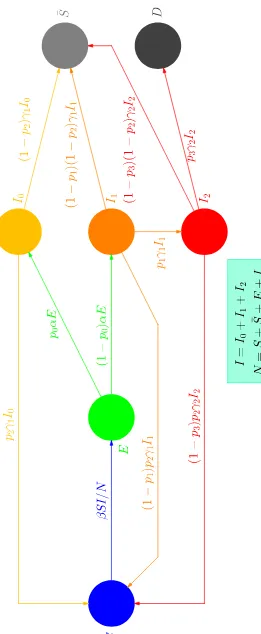
The first compartmental models in Epidemiology are approximately one cen-tury old. A good review of the efforts to model the dissemination of infectious diseases may be found in Ref. [2]. This note will be kept as short as possible, containing only what (in my judgement) is relevant to the model which is put forward in this study in order to account for the dissemination of the COVID-19 disease (and of similar diseases). The transfer diagram of this model is displayed in Fig. 1.
2.1 Definitions
At a given time, each subject is categorised into one of the following seven groups:
• The ‘susceptible’ subjects (S) are those who can be infected.
• The ‘exposed’ subjects (E) are those who have been infected, but are not
yet infective themselves.
• The ‘asymptomatic infective’ subjects (I0) are those who have been infected, but - whichever the reason - are not symptomatic.
• The ‘symptomatic phase-I infective’ subjects (I1) are infective subjects who are developing weak symptoms.
• The ‘symptomatic phase-II infective’ subjects (I2) are infective subjects who are developing strong symptoms (necessitating hospitalisation).
• The ‘immune’ or ‘unsusceptible’ subjects ( ¯S) are those who have recovered with immunity, as well as those who might have been immune to the disease in the first place.
• The ‘deceased’ subjects (D) are those who did not survive the phase II of
the disease.
Evidently, these seven populations 1 depend on time t. Two remarks need
to be made. a) At this time, it remains unknown whether the asymptomatic subjects are infectious [3], how much infectious they might be, and for how long; they will be treated here as equally infectious (and for an equally long
temporal interval) as if they had been I1 subjects (who recover from the
dis-ease). b) It remains unknown whether (at least in some cases) recovery from the COVID-19 disease induces immunity against the virus; also unknown is for how long such immunity might last.
1 For the sake of brevity, the same letters will be used henceforth, to identify both
In this form (to be referred to as ‘simplified version’ henceforth), the model contains neither the vital dynamics (i.e., no births or deaths due to other causes) nor the effects of vaccination; the full version of the model, containing both effects, is outlined in Appendix A. Like most compartmental models, this model may be applied to the entire human population within a region of interest (identified herein as one sovereign country) or to subgroups of that population.
The discussion will be facilitated if, prior to entering the details, some addi-tional definitions are given. As far as the early development of the disease for one infected subject is concerned, three are the important moments:
• the instant t1 at which the subject becomes infected,
• the instant t2 at which the subject becomes infective, and
• the instant t3 marking the onset of symptoms.
(For some diseases,t2 > t3: an infected subject becomes infective after the on-set of symptoms. In the case of the COVID-19 disease, there are indications of pre-symptomatic transmission.) Were the development of such diseases iden-tical for all infected subjects, an infector and a related infectee would follow time-shifted, yet identical, timelines: ift1,t2, andt3were the infector’s timeline characteristics, those of the infectee would be: t′
1 =t1+ ∆t, t
′
2 =t2+ ∆t, and t′
3 =t3+ ∆t, where the constant temporal interval ∆t ≥t2−t1 (and smaller than the temporal interval during which the infector remains infectious). How-ever, neither the infection-to-infectiousness (t2−t1) nor the incubation (t3−t1) interval may be thought of asδ-distributed quantities; in case of the COVID-19 disease, broad distributions have been established. To describe the character-istics of the dissemination of infectious diseases, Epidemiology makes use of three temporal intervals:
• the incubation interval t3−t1 (defined for each subject),
• the onset-to-onset interval (serial interval)t′
3−t3 (defined for each infector-infectee pair), and
• the infection-to-infection interval (generation interval) t′
1 −t1 (defined for each infector-infectee pair).
One would expect that a) these three intervals are positive and b) the serial and generation intervals are equal. In reality, only the incubation and gen-eration intervals are positive; negative estimates for the serial interval have appeared, implying that - on occasion - the infectee develops symptoms be-fore the infector does; in the case of COVID-19, a number of studies [4–6] report on distributions of the serial interval with substantial negative tails.
A weighted average for the incubation interval for the COVID-19 disease may
average for the serial interval 2 may be obtained from Refs. [4–7,11,13,16–18]
as 4.35(25) d. Compared to a ‘paired’ analysis, any difference between the
mean incubation and serial intervals might be ‘washed out’ when averaging is performed. However, even after considering the studies which reported results
on both intervals, consensus does not seem to emerge 3.
2.2 The model parameters
In its simplified version of Fig. 1, the model contains ten parameters, and applies to the short-term (spanning temporal intervals of - typically - a few months) dissemination of diseases (or recurring cycles of diseases) for which no vaccines are available. To be able to model the dissemination of diseases which develop over longer time scales, the model would need enhancement, see Appendix A.
The parameters in the simplified version of the model are:
• Parameter α is the rate parameter involved in the exponential decrease of
the population of the exposed E, provided that the transmission process
ceases. As very few results on the generation interval (which should be
associated with α) are available at this time, α will be taken to be the
inverse of the average serial interval.
• Parameter β (infection rate). Being the product of the average number of
contacts per subject per unit time and the probability of virus transmission in a contact between an infective and a susceptible subject, this parameter may be thought of as the propellant in the outbreak of the disease.
• Parametersγ1,2. These two parameters regulate the rates at which the
pop-ulationsI1 and I2, respectively, would diminish, were they not replenished
by new infections. The decrease in the I1 population is due either to the
recovery of the subject or to the development of strong symptoms (in which
case, the subject enters the phase II of the disease and the I2 population).
The decrease in theI2 population is due either to the subject’s recovery or
to the subject’s death.
2 A critical review of the existing literature for the serial interval may be found
in Ref. [15], which concludes that the value of about 6.6 d has the best chances to account for the data from European countries. Although the argumentation in Ref. [15] (e.g., on the variability of the social contact across countries) may be valid, I decided to estimate the average serial interval using ‘world’ data.
3 Tindale and collaborators concluded that the infection was transmitted (on
• Parameterp0 is the fraction of the exposed who become asymptomatic
in-fective subjects (E → I0). The remaining subjects, departing from group
E, enter the I1 population.
• Parameter p1 is the fraction of the symptomatic phase-I infective subjects
who enter the phase II of the disease (I1 →I2).
• Parameterp2 is the fraction of the recoveries without immunity.
• Parameterp3 is the fatality rate, defined here 4 as the fraction of the
symp-tomatic phase-II infective subjects who do not recover (I2 →D).
Two remarks are due. a) From the point of view of the infectiousness and the recovery rate, the asymptomatic infective subjects are treated as if they were symptomatic phase-I infective subjects; unlike in Ref. [19], it will not
be assumed here that the I0 subjects are less infectious than the subjects of
the other two infective groups I1 and I2. b) The recoveries without immunity
involve the same probability (p2) regardless of the type of the recovered subject (i.e., whether that subject originally belonged to the I0, I1, or I2 group).
The most essential factor in the dissemination of a disease is how the trans-mission compares to the recovery rate. Evidently, if the former is larger, the disease spreads; otherwise, it dies off with time. The aggressiveness of a virus is encoded in the ratioβ/γ, identified in Epidemiology as the basic reproduction
number R0 (also known as transmissibility). In this study, R0 will be the
ba-sic reproduction number, the property associated with the free dissemination
of the disease, i.e., in the absence of any mitigation measures or (in general) enforced/spontaneous modification of the social behaviour of the subjects. On the contrary, the transmissibility of the disease in an environment where re-strictions apply (either due to measures imposed on the social activities of the subjects or due to modification of the social behaviour of the subjects as the disease spreads) will be the effective transmissibility, a time-dependent
quan-tity, and will be denoted by R. The effectiveness of the mitigation measures
in controlling the dissemination of the COVID-19 disease has been addressed in Ref. [20].
Under these definitions, it follows that a disease tends to spread if R > 1, whereas it tends to wane if R <1. The sole aim of the mitigation measures is
to bring R to values below 1, and - desirably - make it as small as possible.
The only parameter which pertains to human behaviour (and may therefore be modified) isβ. Isolation and restrictions in movement aim at reducing the number of contacts per subject per unit time, whereas the social distancing
4 Several quoted fatality rates in the case of the COVID-19 disease are misleading,
aims at reducing the probability of the virus transmission per contact. Either way, β is reduced, resulting (under constant γ) in a reduction in R. In this work,R will be identified as the ratioβ/γ1, whereβ may be thought of as the effective infection rate, as opposed to the constantβ0 which is a characteristic of each virus.
At the beginning of this section, it was mentioned that the simplified version of the model contains ten parameters, yet eight have been listed thus far. The last two parameters enter the empirical modelling of the effective transmissibility.
The effect of the dissemination of a life-threatening disease is the inevitable increase in the cumulative number of fatalities with increasing time. Mitigation measures aim at disrupting the transmission process of the virus, hence at reducing the number of new infections, hence at reducing the number of new fatalities. Evidently, the reduction in transmissibility may be thought of as due to the imposition of the mitigation measures or to modification of the social behaviour of the subjects as a result of the rise in the exposure to danger, intensifying with increasing cumulative number of fatalities. My thesis is that what drives the reduction in transmissibility, the cause or the effect, is of no relevance: the important issue is the association between the reduction in transmissibility and the cumulative number of fatalities within each country. To be able to compare the results across countries, the number of fatalities per country must be normalised to the population of that country; equivalently, one may reduce the number of fatalities to a fixed population, sayn= 100 000 subjects, an option which will be followed here. If the cumulative number of fatalities in the initial populationN(0) isD, then the number of fatalities per
n subjects is d = Dn/N(0). The factor (to be applied to R0 in order that
R(t), equivalently β(t), be extracted) should be 1 at t = 0 (in the analysis,
D(0) = 0) and continue to be equal to that value provided that D < 1. One
may argue that the reduction in transmissibility commences at the moment of the first fatality, i.e., when d=dmin =n/N(0). The simple form
R(d) =Rf + (R0−Rf) exp (−ζ(d−dmin)) , (1)
applicable for d > dmin, was found to work reasonably well. The quantities
Rf and ζ are adjustable (free) parameters; Rf would be the transmissibility
if dcould reach infinity; ζ−1 is related to the number of fatalities (per 100 000 subjects) which would be required so that the transmissibility drop to the
average of R0 and Rf. One additional consideration, however inessential as
(fortunately) d ≪ n in this work, must be taken into account. In reality,
R(n) must identically vanish, as the equality d=n implies that there are no susceptible subjects to whom the disease could be transmitted. To be able to take this condition into account, the aforementioned curve R(d) for Rf ≥
0 will be followed up to the point d = d0 from where the tangent to the
then be followed from d=d0 up to the point (n,0). (Of course, R(d) = 0 for d > n.) If Rf <0, the aforementioned curve R(d) will be followed up to the
minimal value between the 0-crossing dmin −ζ−1ln (−R
f/(R0−Rf)) and n,
above whichR(d) will be set to 0. The quantityd0may be obtained iteratively when Rf >0 (the convergence is very fast), using the scheme
d0 =dmin− 1
ζ ln
Rf
(R0 −Rf) (ζ(n−d0)−1)
!
,
whereas analytical solutions are available for Rf ≤ 0. It needs to be
empha-sised that this correction to Eq. (1) was applied on account of principle and mathematical rigour; to all intents and practical purposes, Eq. (1) suffices.
All model parameters (save for Rf) are non-negative; furthermore, the
prob-abilities p0,...,3 ≤ 1. In principle, Rf > 0, though it cannot be excluded that,
Rf being an effective parameter, some data might prefer a negativeRf value.
2.3 Time evolution
The transfer diagram of Fig. 1 leads to the following system of first-order ordinary differential equations (ODEs).
˙
S =−βSI/N +p2γ1I0 + (1−p1)p2γ1I1+ (1−p3)p2γ2I2 ,
˙¯
S = (1−p2)γ1I0+ (1−p1)(1−p2)γ1I1+ (1−p3)(1−p2)γ2I2 , ˙
E =βSI/N −αE ,
˙
I0 =p0αE −γ1I0 ,
˙
I1 = (1−p0)αE−γ1I1 , ˙
I2 =p1γ1I1−γ2I2 ,and
˙
D=p3γ2I2 , (2)
where the dots indicate time derivatives, I =I0+I1 +I2 is the total number
of infective subjects, and N =S+ ¯S+E+I is the total number of subjects who are alive at a given time. For fixed parameters, the time evolution of the seven populations may be obtained via standard methods. The fourth-order
Runge-Kutta method with a constant increment of 10−4 d (i.e., 8.64 s) was
used, see Ref. [21], pp. 907–910.
2.4 Data
experimental data. At first, I thought that the number of new infections in each country could be used as input, but this option was abandoned, as it
gradually became clearer that the confirmed cases represent a fraction of the
true amount of the infective subjects I; theI0 subjects will not visit a doctor (let alone take any test), and the same goes for many of those who belong to the
I1 group: weak symptoms point to common cold or influenza. I therefore came
to disregard the number of new infections as providing credible information. (For the same reason, I find the recovery rates equally unreliable.)
There are two additional reasons why the new infections are not fit for use.
• During the outbreak of the disease, the number of diagnostic tests,
per-formed daily within each country, generally increased with time. In an envi-ronment where not everyone can be tested, the consequence of an increasing number of tests from day to day is an increasing number of new infections, even for a constant number of infected subjects. As there is little or no information about how many tests are performed in each country on a spe-cific date, infection rates (positive tests normalised to the total number of tests performed) can hardly be estimated. In addition, ‘quantum steps’ in the number of tests from day to day (e.g., due to the availability of a more effective test on a specific date) introduce discontinuities in the distribution of the new infections and reduce the reliability of these data further. One may argue that, unless reliable tests are made on random samples of the population in each country (in accordance with the principles of Sampling Theory), the fraction of the infective subjects (in one country, at one time) will remain unknown.
• New infections refer to the time when tests are made and turn out positive,
not to the time when the infections truly occur. A symptomatic subject will show the first symptoms after the (broadly-distributed) incubation interval elapses, and might wait for a few additional days (during the phase I of the disease) before seeking medical consultation; it is unlikely that any tests are performed within one week of the infection date. As a result, a delay of several days is certainly to be expected between the time instants when new infections truly occur and when they are discovered, consequently reported. To summarise, yesterday’s reported new infections are not ‘new’ at all; they are one to two weeks ‘old’, perhaps even older. As a result, any analysis of new-infection data must account for this delay.
It then dawned on me that, in all probability, the most reliable piece of in-formation in each country is the number of new fatalities or their cumulative
numberD. I decided to make use of the latter and apply the model in the case
fatality 5. The input-cutoff date in this study is April 30; for the sake of ver-ification, the input data were inspected on May 4, May 28, and June 8. The last inspection revealed extensive corrections in the case of the dataset from the US, spanning several weeks, and also affecting the entries in April [22]. Due to this revision, the number of fatalities by the input-cutoff date were increased (in that dataset) by 162. As a consequence, all fits to the data from the US had to be (and were) made anew; this version of the study represents the up-to-date status, also taking into account the corrections applied to the input dataset from the US sometime between May 28 and June 8.
There are two reasons why I avoided using the global data on the fatalities due to the disease.
• The mitigation measures against the dissemination of the disease were taken
by sovereign countries, not at the international level.
• The disease reached different parts of the globe at different times. In
or-der to make meaningful use of the global data, one would have to shift each dataset in time. However, even this operation might not be sufficient. To explain quickly why I do not consider the use of the global data (even after the shifting in time) meaningful, I will refer to the cumulative distri-bution of new infections and fatalities in Greece and in Switzerland, two European countries with comparable population; these two countries re-ported their first infections with one day of difference (February 26 and 25, respectively) and their first fatalities within one week (March 12 and 5, respectively). By April 30, 2 591 subjects had been confirmed as COVID-19-positive in Greece; 29 586 in Switzerland. By that time, Greece counted 140 dead; Switzerland 1 737. With hindsight, the dissemination of the dis-ease in each country depends on a variety of factors, namely the timing of the mitigation measures, the efficiency of the healthcare system, the avail-ability of tests, the population density, the social behaviour, the level of cross-border labour mobility (which, in my judgement, had the biggest im-pact in the aforementioned comparison between Greece and Switzerland), etc. Although the same argument also holds for the counties, provinces, de-partments, states within one country, their differences are expected to be less prominent than those across sovereign countries.
There are some unexplained features in the data, as they are given in Ref. [22], namely the appearance of daily spikes which are well beyond the statistical fluctuation, as the case is for the number of fatalities in France in a few days in April. There is no doubt that the mis-assignment of fatalities is possible (assessed as COVID-19-related, though unrelated in truth; not assessed as COVID-19-related, though related in truth). The situation worsened in May;
5 The first fatality was a Chinese tourist who was hospitalised on January 28 and
some reported values of new infections and fatalities were even negative (e.g., see the number of new infections in France on May 26 and in Spain on May 25, and the number of new fatalities in France on May 19 and in Spain on May
25), indicating ‘aggregated’ corrections to the cumulative number of cases,
thus circumventing the trouble of applying the appropriate corrections to the past daily data.
2.5 Optimisation
For the optimisation, the MINUIT software package [24] of the CERN library was used. The MINUIT software package is the standard in Particle Physics, and its robustness has been tested and proved during four decades of appli-cation. Other of its advantages include that it is freeware, it is downloadable from a safe site, and it is available in two versions: FORTRAN (the version used here) and C/C++.
Each fit involved four minimisation methods: SIMPLEX, MINIMIZE, MI-GRAD, and MINOS.
• SIMPLEX uses the simplex method of Nelder and Mead.
• MINIMIZE minimises the user-defined function, see Eq. (3), by calling
MI-GRAD, but reverts to SIMPLEX in case that MIGRAD fails to converge.
• MIGRAD is the workhorse of the MINUIT software package. It is a
variable-metric method, also checking for the positive-definiteness of the Hessian matrix.
• MINOS performs a detailed error analysis, separately for each free
param-eter. Given that it takes into account the non-linearities in the problem, as well as the correlations among the model parameters, MINOS yields reliable estimates for the fitted uncertainties.
For a fixed parameter vector and initial populations S(0), ¯S(0), E(0), I0(0), I1(0), I2(0), and D(0), the system of ODEs of Eq. (2) is solved, yielding the seven populations S(t), ¯S(t), E(t), I0(t), I1(t), I2(t), and D(t) up to time t, representing the sum of two temporal intervals: the first interval is the time required for D(t) to reach the first fatality/fatalities in the input dataset, whereas the second interval reflects the temporal span of the specific dataset. As the fatalities are reported daily, the following minimisation function has been implemented:
χ2 =
M
X
i=1 (Dth
i −D
exp
i )2/D
exp
i , (3)
where Dth
i is the fitted value (corresponding to the solutionD(t) for the i-th
day in the dataset), Diexp is the corresponding observation (the cumulative
dimension of the Dthi ,exp arrays. Equation (3) assumes that the uncertainty
of Diexp is of the square-root-of-N type (underlying Poisson distribution). The
elements Dth
i depend on the model parameters. The function of Eq. (3) is
submitted to minimisation and the free parameters are varied (internally by
MINUIT) until the χ2 minimum is reached. Apart from the important results
of each fit (i.e., the minimal χ2 value, the fitted values and uncertainties of the model parameters, the Hessian matrix), the MINUIT software package also outputs (by default) a full report, containing the important results obtained in the intermediate steps of the optimisation. To ascertain the successful ter-mination of the application and the convergence of its methods, the report file was routinely inspected.
3 Results
In this study, all results are accompanied by 1σuncertainties, the standard in Physics, representing a confidence interval (CI) of≈68.27%. To transform the results into corresponding to 95% CI, a routinely-used value in several other
scientific domains, one must multiply the quoted uncertainties by ≈ 1.96. If
exceeding 1, the Birge factor qχ2/NDF, which accounts for the quality of
each fit, was applied to the fitted uncertainties; NDF denotes the number of degrees of freedom in each case, i.e., the number of input datapoints minus the number of free parameters in that fit.
3.1 Fixation of the model parameters
As only the cumulative number of fatalities will be fitted to, efforts need to be made to fix as many parameters as possible from external sources; the data cannot determine more than three parameters (and, of course, also the question of which three parameters are varied is relevant).
• Parameter α. Using the average serial interval, extracted from Refs. [4–
7,11,13,16–18] (see end of Section 2.1), one may obtain:α = 0.230(13) d−1.
• Under constant γ1, the variation of R0 is equivalent to that of the model
parameterβ. A compilation of earlyR0 estimates in the case of the
COVID-19 disease may be found in Ref. [25]. In Ref. [26], the reported R0 range
(1.4−3.8) corresponded to 90% CI. A similar result was extracted in Ref. [7]: R0 was restricted in the 1.4−3.9 interval with 95% confidence. In Ref. [27],
Tang and collaborators obtained a large R0 value after making use of an
Singa-pore (average value: 1.97, ranging from 1.45 to 2.48 with 95% confidence), the other for Tianjin (average value: 1.87, ranging from 1.65 to 2.09 with 95% confidence). A more accurate result was obtained in Ref. [18], the
av-erage value 1.94 being accompanied by a 1σ uncertainty well below 0.1.
Although an R0 value was not explicitly reported in Ref. [28], one may
obtain R0 ≈ 3.42 from the authors’ Fig. 2, along with an estimated 1σ
uncertainty of ≈ 0.07, i.e., a value which appears to be compatible with
the effective transmissibility values, extracted in Ref. [20] using data from Wuhan, China, before January 23 (see Fig. 4 therein). Finally, assuming a
serial interval between 6 and 9 d, a broaderR0 distribution was favoured in
Ref. [14], theR0 range extending between 3.8 and 8.9 with 95% confidence.
With such an abundance of R0 results, one might have expected that the
fixation of this parameter would be straightforward. Unfortunately however,
the minimal χ2 value of the reproduction of these R0 results by one
con-stant is about 413.77 for seven degrees of freedom, or 59.11 per degree of freedom, enormous by all standards; one can hardly believe that the
afore-mentioned studies report on the same quantity. Undoubtedly, theR0 results
are model-dependent; consequently,R0 must be treated as a free parameter.
In the optimisation, the (unweighted) average of 3.3 of the values reported in Refs. [7,11,14,18,26–29] will be used as initial guess forR0, and the square root of the unbiased variance of the same values (1.8) as a generous initial guess for theR0 uncertainty.
• Parameters γ1,2. A ballpark estimate of the values of these two parameters was contained in the WHO Director-General’s opening remarks at a briefing on February 24 [30]: “for people with mild disease, recovery time is about two weeks, while people with severe or critical disease recover within three to six weeks.”
To obtain the recovery interval in the case of weak symptoms, four estimates for the time between the onset of the illness and hospitalisation have been used; the hospitalisation was taken as indication that the phase I of the disease was completed without obvious recovery. Of the four estimates, - two came from Ref. [7]: average value 12.5 d, ranging from 10.3 to 14.8
d with 95% confidence (data before January 1), and average value 9.1 d,
ranging from 8.6 to 9.7 d with 95% confidence (data between January 1
and 11);
- one from Ref. [13]: average value 4.4 d, entire distribution from 1 310 cases
ranging from 0.0 to 14.0 d with 95% confidence (data between December
24 and 27, 2019); and
- one from Ref. [14]: average value 5.5 d, ranging from 4.6 to 6.6 d with 95% confidence (data before January 18).
One thus obtains a recovery interval for the phase I of the disease, T1 =
4.98(90) d, and from that result: γ1 = 0.201(36) d−1
.
the illness and the conclusion of the hospitalisation, i.e., recovery or death 6 of the subject, were used:
- one from Ref. [9]: average value 15.0 d, ranging from 12.8 to 17.5 d with 95% confidence (data from hospitalisation to death);
- two from Ref. [31]: average value 18.0 d, entire distribution from 54 cases ranging from 15.0 to 22.0 d with 50% confidence (data from hospitalisation
to death), and average value 22.0 d, entire distribution from 137 cases
ranging from 18.0 to 25.0 d with 50% confidence (data from hospitalisation to recovery);
- one from Ref. [18]: average value 20.0 d, ranging from 17.0 to 24.0 d with 95% confidence (data from hospitalisation to death); and
- one from Ref. [14]: average value 16.1 d, ranging from 13.1 to 20.2 d with 95% confidence (data from hospitalisation to death).
The weighted average of Tt = 20.2(1.2) d is thus extracted. To be able to
obtain γ2, one must subtract from this estimate the recovery interval of
the phase I, in which case the characteristic time scale for the development of the phase II of the disease would be 15.2(1.5) d, which finally yields γ2 = 0.0658(66) d−1.
• Parameterp0. To the best of my knowledge, Mizumoto, Kagaya, Zarebski,
and Chowell [3] were the first to report onp0; their result came from an anal-ysis of data acquired on board of the Diamond Princess cruise ship. In their work, the number of true asymptomatic was inferred from the time evolu-tion of the ratio of the confirmed subjects who had developed symptoms (by a given time) to those who had not; their result was a true asymptomatic population of 113.3 out of 634 confirmed cases, resulting inp0 = 17.9(1.2)%. More recently, the results of an analysis of five studies of the fraction of the asymptomatic subjects appeared [32]: the authors came up with a total of 65 asymptomatic subjects out of 413 confirmed cases, yieldingp0 = 15.7(1.8)%.
Although the two p0 results agree within the uncertainties, the estimate of
Ref. [3] was not used in Ref. [32] on account of principle (as aforementioned, the true asymptomatic population was inferred in Ref. [3], not established
via medical examination). I will extract a p0 estimate from all six studies:
summing up the entries of Refs. [3,32], one obtains 178.3(10.7) expected
true asymptomatic subjects in a sample of 1 047 confirmed cases, yielding p0 = 17.0(1.0)%.
• Parameter p1. According to Ref. [33], 8 255 of 44 415 confirmed cases
ex-hibited strong symptoms; this corresponds to 18.59(18)% of the confirmed
cases. Ap1 result was also obtained in Ref. [10]: 173 out of 1 099 confirmed
cases exhibited strong symptoms; their p1 value (15.7(1.1)%) is somewhat
lower than that of Ref. [33]. By summing up the corresponding entries in these two studies, one obtainsp1 = 18.52(18)%.
• Parameter p2. Very little is known about this parameter, but (owing to
6 As the phase II of the disease is regulated by one rate parameter (γ
the shortness of the follow-up time - the outstanding majority of the orig-inally susceptible subjects remain unexposed) its impact on the results is deemed minor. According to a recent scientific communication by the WHO [34], “there is currently no evidence that people who have recovered from COVID-19 and have antibodies are protected from a second infection.” Given the expected near insensitivity of the main results of this study to
p2, the parameter was originally fixed to 1 (no recovery with immunity).
However, I decided to opt for p2 = 0.90(5), allowing for a small fraction of
recoveries with immunity. Although the odds are not in favour 7, knowing
more aboutp2 will be helpful in fighting the long-term development of the
disease (i.e., potential recurrent cycles of the pandemia).
• Parameter p3. According to Ref. [33], 1 023 out of 44 672 confirmed cases
resulted in the subject’s death. As 8 255 out of 44 415 confirmed cases devel-oped strong symptoms, the probabilityp3 is 1 023·44 415/(8 255·44 672) = 12.32(40)%.
• ParametersRf and ζ will be varied. After analysing the results of ten fits to
the five datasets of this work, the initial guesses for the average value and uncertainty of the parameter Rf were fixed to 0.22 and 0.20, respectively;
of the parameter ζ to 0.78 and 0.40, respectively.
One last remark is due. In Ref. [35], a simple compartmental model with three groups (SIR) was proposed for the dissemination of the COVID-19 disease.
Given the two recovery rates of this work, the recovery rate γ of Ref. [35]
may be thought as an effective one, related to the quantities γ1,2 (hence to
T1 and Tt) of this work. To obtain an effective recovery rate herein, one must
first obtain an effective recovery time, e.g., Teff = (1−p1)T1 +p1Tt; using
the average values and uncertainties of T1, Tt, and p1, as detailed above, one
extracts:Teff = 7.80(77) d. The suggested value in Ref. [35], namely 8.05 d, is in good agreement with the Teff result of this work.
In summary, all the model parameters can be fixed from external sources, save for those three (to be specific, R0, Rf, and ζ) which determine the effective
transmissibility.
3.2 Description of the input data, optimal values of the free parameters
Each call to a MINUIT method generates a growth scenario; in each case, the initial populations ¯S,I0,I1,I2, andDare set to 0, and the number of exposed subjects E(0) is set to 10−7N(0); of course, S(0) = (1 −10−7)N(0). (The
7 Belgium has suffered the highest number of infections (and fatalities) per capita
populations N(0) of the five countries are fixed to estimates obtained in 2019
or 2020.) Therefore, the disease is assumed to start spreading (at t= 0) from
≈ 33 exposed subjects in the US, from 6 in Italy, etc. Either these subjects
became infected in their respective countries (e.g., via contacts with infective tourists) or after a trip abroad; the details of the exposures are irrelevant. The system of ODEs of Eq.(2) is solved, yieldingS(t),E(t),I0(t),I1(t),I2(t), ¯S(t), and D(t) att >0; after the first fatality, the effective transmissibility R(d) of Eq. (1) is used in the calculation.
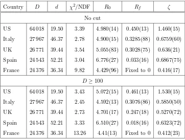
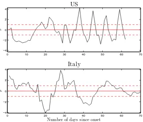
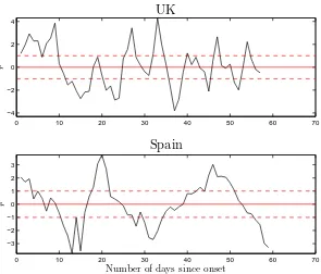
The important results of the fits to the five datasets of this study are given in Table 1 (upper part), whereas Figs. 2-4 show the time dependence of the normalised residuals of the fits to the five datasets (given the range of the input data, plots of input and fitted values are not particularly revealing to
the naked eye, e.g., see Fig. 5 for the data from the US). As the reduced χ2
values of Table 1 and Figs. 2-4 demonstrate, the quality of the fits is poor in the pure statistical sense. A few remarks on the five datasets follow.
• Regarding the data from the US, an undulating behaviour is noticeable in
the reported number of new fatalities (the same goes for the corresponding
data from the UK), with typically 3−5 d of systematically more reported
fatalities, followed by 2−3 d of fewer incidents.
• The dataset from Italy is best described with the model.
• The data from Spain pose some questions; the transmission of the virus
appears to have been faster there: the number of fatalities rises more sharply with time (than in the other four countries) and approaches saturation faster.
• There is considerable fluctuation in the data from France; that dataset is
worst described with the model. The data in the first half of April contain several spikes. The result of these fluctuations on the description of the input data is an unavoidable rise in theχ2 values of the fits.
There are established ways to smooth ‘noisy’ data (e.g., LOESS, LOWESS, the Savitzky-Golay filter, the application of running-average windows, etc.). However, I decided to avoid applying any kind of smoothing algorithm and to continue instead to use the original values, as they appear in Ref. [22].
The analysis was repeated after removing from the input datasets the dat-apoints with fewer than 100 fatalities. This way, the relative uncertainty in each input datapoint does not exceed 10%. It was found that this cut has no sizeable impact on the results, see Table 1, lower part. Therefore, the low-N fluctuations cannot be blamed for the general poorness of the quality of the fits.
Table 1
The results of the fits of the model to the five datasets used as input (upper part: results from the analysis of the entire datasets; lower part: accepted in the analysis were only the entries exceeding 99 fatalities). The countries are listed in descending order of the fatalities reported by the input-cutoff date in this study (April 30). The first column identifies the country. The second column represents the cumu-lative number of fatalities D, whereas the adjacent column gives the number of fatalities dper 100 000 subjects (see end of Section 2.2) in that country. The last four columns contain the reduced χ2 values of the each fit (χ2 per degree of free-dom), and the fitted values and uncertainties of the free parametersR0,Rf, andζ.
(The fitted uncertainties of the parameters in the MINUIT output represent stan-dard errors of the means.) In each fit, the remaining model parameters were fixed to the corresponding central values as detailed in Section 3.1. For the fits to the data from France,Rf was set to 0.
Country D d χ2/NDF R
0 Rf ζ
No cut
US 64 018 19.50 3.39 4.980(14) 0.450(13) 1.460(15)
Italy 27 967 46.37 2.78 4.900(15) 0.3285(88) 0.6759(60)
UK 26 771 39.44 3.54 5.055(83) 0.3028(75) 0.636(21)
Spain 24 543 52.21 3.04 6.776(27) 0.033(16) 0.6867(75)
France 24 376 36.34 9.82 4.429(96) Fixed to 0 0.416(17)
D≥100
US 64 018 19.50 3.43 5.072(15) 0.461(13) 1.530(15)
Italy 27 967 46.37 2.45 4.592(13) 0.3076(86) 0.5850(50)
UK 26 771 39.44 2.73 4.701(17) 0.247(18) 0.5270(72)
Spain 24 543 52.21 3.33 6.510(27) 0.018(16) 0.6323(72)
France 24 376 36.34 13.26 4.41(13) Fixed to 0 0.412(23)
put forward. One hundred combinations of random, normally-distributed, un-correlated values for these parameters were generated, using the results for the central values and the uncertainties according to Section 3.1. Each such combination was used in one fit to the data from one country; as a result, twenty fits per country were performed. The important results (i.e., a coun-try identifier, the minimal χ2, the NDF, the current values of the seven fixed parameters, as well as the results for the fitted values and uncertainties of the free parameters) were stored in binary files for later processing.
The parameter Rf was fixed to 0 in the fits to the data from Spain and
0 10 20 30 40 50 60 70 −4
−2 0 2 4
r
US
0 10 20 30 40 50 60 70
−4 −2 0 2 4
Number of days since onset
r
Italy
Fig. 2. Description of the input data with the compartmental epidemiological model of Fig. 1, for the central values of the fixed parameters as detailed in Section 3.1, and for the fitted values of the free parameters from Table 1. The quantity
ri = (Dthi −D
exp
i )/ p
Diexp is the normalised residual of thei-th datapoint. The hor-izontal axis contains the number of days since the first fatality in each country. The plots correspond to the data from the US (upper part of the figure) and Italy (lower part of the figure). The last datapoint in each plot represents the entry on April 30. The horizontal lines have been included for eye guidance; the solid straight line corresponds to the ideal description (r = 0), whereas the two dashed lines delineate the statistical expectation |r|= 1.
cannot be evaluated or does not come out as expected (i.e., positive definite).
After this fixation, no problems were found in the fits. The twenty R0 values
and fitted uncertainties for each country were analysed further; to avoid the introduction of bias into the results due to any small fitted uncertainties, a median uncertainty was evaluated (per country) and replaced those of the fitted uncertainties (in the results of that country) which were short of that median value. A weighted average was next extracted for each country, along
with the rms (root-mean-square) of the R0 distribution, see Table 2.
The five average R0 values of Table 2 may be thought of as ‘independent
ob-servations’. The grand mean was obtained from these values and the standard error of the means was assigned to the grand mean as final uncertainty. The main result of this work is
0 10 20 30 40 50 60 70 −4
−2 0 2 4
r
UK
0 10 20 30 40 50 60 70
−3 −2 −1 0 1 2 3
Number of days since onset
r
Spain
Fig. 3. Same as Fig. 2 for the data from the UK (upper part) and Spain (lower part).
0 10 20 30 40 50 60 70
−10 −5 0 5 10
Number of days since onset
r
France
0 10 20 30 40 50 60 70 0
1 2 3 4 5 6 7x 10
4
Number of days since onset
D
Data from the US
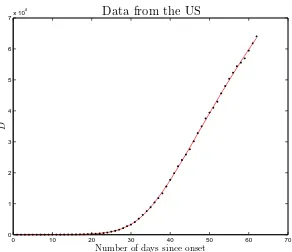
Fig. 5. Comparison between input and fitted values for the cumulative number of fatalities in the US. Although the visual inspection of this plot leaves a positive impression, the reducedχ2of the fit is equal to 3.37 (see Table 1), indicating a poor description of the input data in the pure statistical sense.
Table 2
Weighted averages and rms values per country for the model parameterR0, obtained from 100 fits (in total) taking account of the effects of the variation of the parameters
α, γ1,2, andp0,...,3 according to Section 3.1. Contained in the second column is the range of theχ2/NDF values of the relevant fits.
Country χ2/NDF R
0
USA 3.37−3.44 4.98(63)
Italy 2.75−2.87 5.01(90)
UK 3.46−3.65 4.90(69)
Spain 2.58−5.56 6.5(1.2)
France 8.04−15.93 4.35(63)
This result lies in between the values reported by Cao and collaborators [29], and by Tang and collaborators [27]. It agrees better with the former result
(even though the R0 value of Ref. [29] is not accompanied by an uncertainty).
The difference to the result of Ref. [27], the largest of the reported R0 values
distribution. The R0 result of this work provides support for the large-R0 thesis in the case of the COVID-19 disease.
It must be mentioned that the scheme used in the empirical modelling of the effective transmissibility might have an impact on the estimate forR0. The re-liable determination of the effective transmissibility in the dissemination of the COVID-19 disease is an interesting subject, which is surely worth additional investigation. One interesting transmissibility-reduction scheme, fine-tuned to the dissemination of the disease in Wuhan, was introduced in Refs. [27,36]. That scheme quantifies the impact of each of the mitigation measures and ap-pears to be generally applicable (after its parameters have been appropriately fixed, separately for each country).
To provide estimates for the effective transmissibility, other methods have been put forward, e.g., see Ref. [37] for a review. One method, which can easily be implemented and requires only the time series of the new infections in each country, was introduced in Ref. [38]; I have already expressed my scepticism about the reliability of the new-infection time series. Within the framework
of that model, the effective transmissibility at time t is shown to follow the
Gamma distribution with parametersaandb, which may be obtained from the
new-infection data between times t−δtandt, whereδt is associated with the distribution of the serial interval. To suppress the fluctuation in the extracted values, a user-defined window may be applied to the input data. The result of the application of the method in the case of the five countries of this work was not satisfactory: the five new-infection time series suggest a power fall-off of the effective transmissibility (large-d behaviour), which had been tried (prior to the implementation of the scheme of Section 2.2), but yielded an inferior description of the five datasets compared to Eq. (1).
The most probable temporal interval between the first exposures and the first fatality in each country may also be derived from the data. The results are:
• 14−16 d for the US (most likely exposures between February 13 and 16;
result of the fit of Table 1, upper part: February 14-15);
• 20−22 d for Italy (most likely exposures between January 30 and February
2; result of the fit of Table 1, upper part: January 31-February 1);
• 19−21 d for the UK (most likely exposures between February 13 and 16;
result of the fit of Table 1, upper part: February 14-15);
• 18−19 d for Spain (most likely exposures between February 13 and 15;
result of the fit of Table 1, upper part: February 13-14); and
10 20 30 40 50 60 0
2 4 6 8 10 12x 10
5
Number of days since onset
N
u
m
b
er
o
f
su
b
je
ct
s
Exposed Infective Phase−II infective Deceased
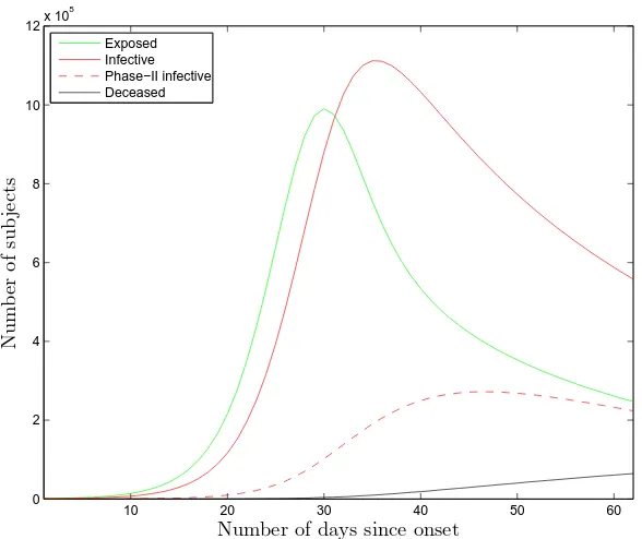
Fig. 6. The time evolution of the populations of four of the groups of the model for the US. The first fatality occurred on February 29. The upper limit in the horizontal axis represents the input-cutoff date in this study, namely April 30.
3.3 Predictions
The results of the optimisation may be used in order to predict the time evolution of the populations of the seven groups of the model. For the sake of example, one obtains Fig. 6 for the time evolution of the groups E, I, I2, and D in the US. For this plot, the parameters α, γ1,2, and p0,...,3 were fixed to their central values as detailed in Section 3.1. The fitted values of R0, Rf,
and ζ for the US were given in Table 1, upper part. An estimate for the total
number of fatalities due to the virus (in fact, for the number of fatalities after
this cycle of the pandemia is over) may be obtained by letting the application
run for an adequately long follow-up time (representing infinity); running the
software for 200 d (up to September 1) yielded the result: D∞≈137 584.
At this time, meaningful uncertainties cannot be assigned to the model predic-tions; the procedure to obtain these uncertainties is straightforward, but has not yet been implemented. However, working uncertainties may be obtained indirectly, after using empirical models in the optimisation, e.g., models based on the log-normal, the Weibull, or the Gamma distribution; such models yield
a relative uncertainty in the cumulative number of fatalities D∞ around 5%.
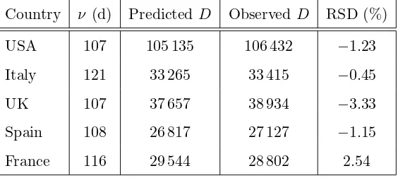
Table 3
The model predictions for the cumulative number of fatalities by May 31, 2020, for the five countries used herein. The observed values were copied from Ref. [22] on June 8. The second column contains the number of days ν between the expected first exposures (generally different for the five countries) and May 31. It must be mentioned again that the predictions were derived from input data before May 1; no data from May were involved in any way in the database used in the optimisation. RSD denotes the relative symmetrised difference (difference between prediction and observation, normalised to their average).
Country ν (d) Predicted D ObservedD RSD (%)
USA 107 105 135 106 432 −1.23
Italy 121 33 265 33 415 −0.45
UK 107 37 657 38 934 −3.33
Spain 108 26 817 27 127 −1.15
France 116 29 544 28 802 2.54
some data which have not entered the optimisation. Selected in this respect was May 31, i.e., one month after the input-cutoff date for the inclusion of data in the five databases of this work. The model predictions for the five countries, along with the actual data on May 31 (copied from Ref. [22] on June 8), are given in Table 3. The differences between the predicted and observed values do not exceed the few-percent level.
It must be emphasised that predictions make sense if the collective behaviour continues to be shaped in accordance to the scheme used in the empirical modelling of the effective transmissibility. If the collective behaviour is modi-fied, be that due to the relaxation of the mitigation measures or to re-adjusted norms following the long-term exposure of the human population to a lasting phenomenon (habituation), any predictions are likely to fail.
4 Conclusions and discussion
The novel part in this work is that it uses only the cumulative number of fatalities due to the disease in each country, i.e., data from the public domain. Given that, due to the unavailability of a fast and reliable diagnostic test, the number of infected subjects remains uncertain, the number of fatalities may be regarded (in my judgement) as the most reliable piece of information regarding this disease. Of course, ‘being the most reliable’ is not synonymous to ‘being reliable’. Although I have not seen scientific studies on the reliability of the reported number of fatalities, several experts (and non-experts) have expressed their scepticism in newspaper and journal articles, in interviews, and in blogs. In some cases, it has been suggested that the true numbers may be as much as 60% higher than those reported [39].
Fits of the model to the data from five countries, namely from those which have been hit most severely by the disease (regarding the number of fatalities), have been performed following a transmissibility-reduction scheme based on the cumulative number of fatalities. An estimate for the basic reproduction
number R0, the most important measure of the aggressiveness of a virus, for
the free dissemination of the COVID-19 disease (no mitigation measures, no modification of the social behaviour of the subjects as a result of the rising death toll) has been obtained:R0 = 4.91(33), see Eq. (4). This result disagrees with several early estimates, and points to a more aggressive virus (than those early estimates had suggested); the result of this work places the COVID-19 disease at equal level with poliomyelitis, rubella, pertussis, smallpox, and distances it from common cold and influenza.
Provided that the future behaviour of the susceptible subjects matches their past behaviour (e.g., regarding social distancing and self-isolation in suspect cases), predictions for the time evolution of the populations of the seven groups of the model may be obtained from the results of the fits.
Last but not least, the reliability of the results extracted herein relies on the validity of a number of assumptions.
• No significant contributions have been left out of the transfer diagram of
the model (see Fig. 1).
• The association between the reduction in transmissibility and the
cumula-tive number of fatalities in each country, as explained in Section 2.2, holds. It might be that the scheme used in the empirical modelling of the effective transmissibility has an impact on the extracted estimate for the nominal transmissibility R0.
• The average values of the model parameters are not sizeably different to the
results detailed in Section 3.1.
• The correctness of the quoted uncertainty in the nominal transmissibility
Acknowledgements
I am indebted to Kenneth McIntosh for answering a few questions regard-ing the asymptomatic infective subjects in the case of the COVID-19 virus; to Megan Murray for answering a question regarding the extraction of the effective transmissibility from the data; and to Marco Ajelli for answering a question regarding Ref. [13]. I am grateful to G¨unther Rasche for his careful reading and valuable comments.
Figure 1 has been created with CaRMetal [40]. The remaining figures have
been created with MATLABR (The MathWorks, Inc., Natick, Massachusetts,
United States).
I have no affiliations with or involvement in any organisation, institution, company, or firm with/without financial interest in the subject matter of this work.
References
[1] https://www.who.int; https://coronavirus.jhu.edu;
https://en.wikipedia.org/wiki/Coronavirus disease 2019;
https://www.uptodate.com/contents/coronavirus-disease-2019-covid-19-epidemiology-virology-clinical-features-diagnosis-and-prevention;
https://ourworldindata.org/coronavirus
[2] H.W. Hethcote, ‘The Mathematics of infectious diseases’, SIAM Rev. 42 (2000) 599–653; available from https://www.jstor.org/stable/2653135
[3] K. Mizumoto, K. Kagaya, A. Zarebski, G. Chowell, ‘Estimating the asymptomatic proportion of Coronavirus disease 2019 (COVID-19) cases on board the Diamond Princess cruise ship, Yokohama, Japan, 2020’, Euro. Surveill. 25 (2020) 2000180.
DOI: 10.2807/1560-7917.ES.2020.25.10.2000180
[4] Z. Du et al., ‘Serial interval of COVID-19 among publicly reported confirmed cases’, Emerg. Infect. Dis. 26 (2020). DOI:10.3201/eid2606.200357
[5] T. Ganyani et al., ‘Estimating the generation interval for coronavirus disease (COVID-19) based on symptom onset data, March 2020’, Euro. Surveill. 25 (2020) 2000257. DOI:10.2807/1560-7917.ES.2020.25.17.2000257
[7] Q. Li et al., ‘Early transmission dynamics in Wuhan, China, of novel Coronavirus-infected pneumonia’, N. Engl. J. Med. 382 (2020) 1199–1207. DOI: 10.1056/NEJMoa2001316
[8] J.A. Backer, D. Klinkenberg, J. Wallinga, ‘Incubation period of 2019 novel coronavirus (2019-nCoV) infections among travellers from Wuhan, China, 20– 28 January 2020’, Euro. Surveill. 25 (2020) 2000062. DOI: 10.2807/1560-7917.ES.2020.25.5.2000062
[9] N.M. Linton et al., ‘Incubation period and other epidemiological characteristics of 2019 novel Coronavirus infections with right truncation: A statistical analysis of publicly available case data’, J. Clin. Med. 9 (2020) 538. DOI: 10.3390/jcm9020538
[10] W. Guan et al., ‘Clinical characteristics of Coronavirus disease 2019 in China’, N. Engl. J. Med. 382 (2020) 1708–1720. DOI: 10.1056/NEJMoa2002032
[11] L.C. Tindale et al., ‘Transmission interval estimates suggest pre-symptomatic spread of COVID-19’, medRxiv: 2020.03.03.20029983.
DOI: 10.1101/2020.03.03.20029983
[12] S.A. Lauer et al., ‘The incubation period of Coronavirus disease 2019 (COVID-19) from publicly reported confirmed cases: estimation and application’, Ann. Intern. Med. 172 (2020) 577–582. DOI: 10.7326/M20-0504
[13] J. Zhang et al., ‘Evolving epidemiology and transmission dynamics of coronavirus disease 2019 outside Hubei province, China: a descriptive and modelling study’, Lancet Inf. Dis. 2020. Published online April 2, 2020. DOI: 10.1016/S1473-3099(20)30230-9
[14] S. Sanche et al., ‘High contagiousness and rapid spread of Severe Acute Respiratory Syndrome Coronavirus 2’, Emerg. Infect. Dis. 26 (2020). DOI: 10.3201/eid2607.200282
[15] J.M. Griffin et al., ‘A rapid review of available evidence on the serial interval and generation time of COVID-19’, medRxiv: 2020.05.08.20095075. DOI: 10.1101/2020.05.08.20095075
[16] S. Zhao et al., ‘Estimating the serial interval of the novel coronavirus disease (COVID-19): A statistical analysis using the public data in Hong Kong from January 16 to February 15’, medRxiv: 2020.02.21.20026559. DOI: 10.1101/2020.02.21.20026559
[17] H. Nishiura, N.M. Linton, A.R. Akhmetzhanov, ‘Serial interval of novel coronavirus (COVID-19) infections’, Int. J. Infect. Dis. 93 (2020) 284–286. DOI: 10.1016/j.ijid.2020.02.060
[19] N.M. Ferguson et al.(Imperial College COVID-19 Response Team), ‘Report 9: Impact of non-pharmaceutical interventions (NPIs) to reduce COVID-19 mortality and healthcare demand’. DOI: 10.25561/77482
[20] A. Pan et al., ‘Association of public health interventions with the Epidemiology of the COVID-19 outbreak in Wuhan, China’, JAMA. Published online April 10, 2020. DOI: 10.1001/jama.2020.6130
[21] W.H. Press, S.A. Teukolsky, W.T. Vetterling, B.P. Flannery, ‘Numerical Recipes: The Art of Scientific Computing’ (3rd edn.), Cambridge University Press, 2007.
[22] Available from https://www.worldometers.info/coronavirus
[23] Available from
https://en.wikipedia.org/wiki/2020 coronavirus pandemic in France
[24] F. James, ‘MINUIT - Function Minimization and Error Analysis’, CERN Program Library Long Writeup D506, CERN, 1998.
[25] Y. Liu, A.A. Gayle, A. Wilder-Smith, J. Rockl¨ov, ‘The reproductive number of COVID-19 is higher compared to SARS coronavirus’, J. Travel Med. 27 (2020). DOI: 10.1093/jtm/taaa021
[26] J. Riou, C.L. Althaus, ‘Pattern of early human-to-human transmission of Wuhan 2019 novel Coronavirus (2019-nCoV), December 2019 to January 2020’, Euro. Surveill. 25 (2020) 2000058. DOI: 10.2807/1560-7917.ES.2020.25.4.2000058
[27] B. Tang, ‘Estimation of the transmission risk of the 2019-nCoV and its implication for public health interventions’, J. Clin. Med. 9 (2020) 462. DOI: 10.3390/jcm9020462
[28] J. Hwang, H. Park, S.-H. Kim, J. Jung, N. Kim, ‘Basic and effective reproduction numbers of COVID-19 cases in South Korea excluding Sincheonji cases’, medRxiv: 2020.03.19.20039347. DOI: 10.1101/2020.03.19.20039347
[29] Z. Cao et al., ‘Estimating the effective reproduction number of the 2019-nCoV in China’,medRxiv: 2020.01.27.20018952. DOI 10.1101/2020.01.27.20018952
[30] Available from https://www.who.int/dg/speeches/detail/who-director-general-s-opening-remarks-at-the-media-briefing-on-covid-19—24-february-2020
[31] F. Zhou et al., ‘Clinical course and risk factors for mortality of adult inpatients with COVID-19 in Wuhan, China: a retrospective cohort study’, Lancet 395 (2020) 1054–1062. DOI: 10.1016/S0140-6736(20)30566-3
[32] O. Byambasuren et al., ‘Estimating the extent of true asymptomatic COVID-19 and its potential for community transmission: systematic review and meta-analysis’,medRxiv: 2020.05.10.20097543.
[33] Z. Wu, J.M. McGoogan, ‘Characteristics of and important lessons from the Coronavirus Disease 2019 (COVID-19) outbreak in China: Summary of a report of 72 314 cases from the Chinese Center for Disease Control and Prevention’, JAMA 323 (2020) 1239–1242. DOI: 10.1001/jama.2020.2648
[34] https://www.who.int/news-room/commentaries/detail/immunity-passports-in-the-context-of-covid-19
[35] J. Sreevalsan-Nair, R.R. Vangimalla, P.R. Ghogale, ‘Analysis of clinical recovery-period and recovery rate estimation of the first 1 000 COVID-19 patients in Singapore’,medRxiv: 2020.04.17.20069724.
DOI: 10.1101/2020.04.17.20069724
[36] B. Tang et al., ‘An updated estimation of the risk of transmission of the novel coronavirus (2019-nCov)’, Infect. Dis. Model. 5 (2020) 248–255. DOI: 10.1016/j.idm.2020.02.001
[37] K.V. Parag, C.A. Donnelly, ‘Optimising renewal models for real-time epidemic prediction and estimation’,bioRxiv: 835181. DOI: 10.1101/835181
[38] A. Cori, N.M. Ferguson, C. Fraser, S. Cauchemez, ‘A new framework and software to estimate time-varying reproduction numbers during epidemics’, Am. J. Epidemiol. 178 (2013) 1505–1512. DOI: 10.1093/aje/kwt133
[39] J. Burn-Murdoch, V. Romei, C. Giles, ‘Global coronavirus death toll could be 60% higher than reported’, Financial Times, April 26, 2020, available from https://www.ft.com/content/6bd88b7d-3386-4543-b2e9-0d5c6fac846c
A The inclusion of vital dynamics
The inclusion of the vital dynamics, as well as of the effects of the vaccination, introduces three additional parameters:
• The birth rate λ in the country under investigation.
• The mortality rate µin the country under investigation.
• The vaccination rate ǫ.
Discarding passive immunity, the complete version of the model rests upon the following system of ODEs.
˙
S =−βSI/N+p2γ1I0+ (1−p1)p2γ1I1+ (1−p3)p2γ2I2−ǫS+λN −µS ,
˙¯
S = (1−p2)γ1I0+ (1−p1)(1−p2)γ1I1+ (1−p3)(1−p2)γ2I2 +ǫS−µS ,¯ ˙
E =βSI/N−(α+µ)E ,
˙
I0 =p0αE−(γ1+µ)I0 , ˙
I1 = (1−p0)αE−(γ1+µ)I1 , ˙
I2 =p1γ1I1−(γ2+µ)I2 ,and ˙
D=p3γ2I2+µN , (A.1)
where I = I1 +I2 +I3 and N = S + ¯S+E +I. This model may be used