and searching biological sequence data
John Norman Hatwell
September 2001
A thesis submitted in part fulfilment of the requirements of the University of London for the degree of Master of Philosophy
Department of Mathematical Biology National Institute for Medical Research
The Ridgeway Mill Hill
All rights reserved
INFORMATION TO ALL USERS
The quality of this reproduction is dependent upon the quality of the copy submitted.
In the unlikely event that the author did not send a complete manuscript and there are missing pages, these will be noted. Also, if material had to be removed,
a note will indicate the deletion.
uest.
ProQuest U643162
Published by ProQuest LLC(2016). Copyright of the Dissertation is held by the Author.
All rights reserved.
This work is protected against unauthorized copying under Title 17, United States Code. Microform Edition © ProQuest LLC.
ProQuest LLC
789 East Eisenhower Parkway P.O. Box 1346
Sequence database searching is a key tool in current bioinformatics. To improve accuracy,
sequence database searches are often performed iteratively: taking the results of one
search as input for the next. The object of this approach being to progressively isolate
increasingly distant relations of the original query sequence. In practice this method works
well when it is supervised by an expert eye' which can determine when an alignment is
good and when sequences should be excluded from it, but attempts to automate this
process have proven difficult. At present PSI-BLAST is one of the few effective attempts,
but a misalignment of sequences or the wrongful inclusion of a sequence will still rapidly
destroy the specificity of the probe, making incorrect matches more likely.
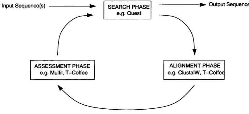
By combining the search program Quest, which is capable of searching a database
using full length multiple sequence alignments, with independent sequence alignment
and assessment programs, we have been able to reduce the occurrence of this problem.
We use a multiple alignment package to generate an accurate alignment of all hits
generated by the Quest program. Sequences that do not appear to 'fit' with the rest of
the alignment are automatically removed by the separate alignment assessment program
Mulfil. The resulting alignment is fed back to Quest for the next iteration. This scheme
In addition, further work demonstrated that equally good quality results are possible
without the use of multiple alignment or profile searching. The Cascade-and-Cluster
scheme uses intermediate sequences and a simple clustering procedure and is able to
produce a result almost equally sensitive and selective as our previous scheme, whilst
Abstract 2
List of Figures 6
List of Tables 7
Abbreviations 8
Acknowledgements 9
1 Introduction 10
1.1 DNA and the Genetic C o d e ... 11
1.1.1 D N A ... 11
1.1.2 The Genetic C o d e ... 13
1.2 The Journey from Gene to Protein... ... 14
1.2.1 Transcription... 15
1.2.2 Translation... 15
1.3 Evolution... 16
1.4 Sequence Databases... 19
1.5 Sequence Comparison & Database Searching... 22
1.5.1 Sequence A lig n m e n t... 22
1.5.2 Database S earching... 32
1.6 A im s ... 44
2 Quest: A Profile Based Search Program 47 2.1 Quest: Method of Operation ... 49
2.1.1 Stage I: Input & Preprocessing... 49
2.1.2 Stage II: Tripeptide Matches & Segment Extension...56
2.1.3 Stage III: Segment Assembly & Sequence Scoring ... 59
2.1.4 Stage IV: Hit Selection & O u tp u t... 63
2.2 Quest: Parameters, Modifiers and R u n -M o d e s... 64
2.2.1 Quest Param eters... 65
2.2.2 Quest M o d ifie rs ... 69
2.2.3 Quest R un-M odes... 70
2.3.1 The Cluster ... 75
2.3.2 MPI ... 76
2.3.3 Simple Parallel Database Searching... 77
3 The QUEST Scheme 81 3.1 The Search P h a s e ... 82
3.2 The Alignment P h a s e ... 83
3.2.1 M U LT A L... 83
3.2.2 C LU S T A LW ... 85
3.2.3 P ra lin e ... 86
3.2.4 T -C o ffe e ... 87
3.2.5 Other A lternatives... 88
3.2.6 The Final Decision... 89
3.3 The Assessment Phase... 91
3.3.1 T -C o ffe e ... 92
3.3.2 M u lfil... 92
3.3.3 The Final Decision... 95
3.4 The Method of Ite ra tio n ... 95
3.5 Cascade-and-Cluster - A New Scheme?...98
4 Benchmarks 105 4.1 M e th o d s ... 108
4.2 Results & Analysis... 110
4.2.1 Benchmarking Q uest... 110
4.2.2 Quest Parameter Effects... 113
4.2.3 Benchmarking the QUEST Schem e...119
4.2.4 Cascade-and-Cluster... 124
4.2.5 PSI-BLAST Version 2: An Improved Challenger ... 127
5 The Quest Server: Our Window on the World Wide Web 132
6 Discussion & Conclusions 139
1.1 Translation... 16
1.2 Comparison of Gap C o s ts ... 26
1.3 Dynamic Programming... 27
1.4 The QUEST Scheme... 44
2.1 Input File Format ... 51
2.2 PSSM C o n structio n... 54
2.3 Segment Extension... 58
2.4 Segment Assembly... 61
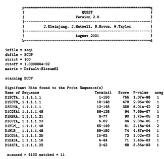
2.5 An Example Quest O u tp u t... 63
2.6 Topology of the Linux C lu ste r... 75
3.1 The Real QUEST Scheme... 97
3.2 A Sequence C lu s te r ... 100
3.3 Cascade-and-Cluster... 102
4.1 Quest Benchmark R e su lts... I l l 4.2 Score Cutoff E ffe c ts ... 114
4.3 Effects of the Strictness P a ra m e te r...115
4.4 Gap Penalty E ffe c ts ... 117
4.5 Benchmarking the QUEST S chem e...120
4.6 Parameter Effects on the QUEST Scheme ...122
4.7 Effects of Alignment Phase on the QUEST Scheme ...123
4.8 Cascade-and-Cluster Benchmark...125
4.9 PSI-BLAST Version 2 ... 128
4.10 PSI-BLAST vs B L A S T P G P ... 130
5.1 The Quest Web Server...134
5.2 Example Results Page: Part I ...136
A Adenine
BLAST Basic Local Alignment Search Tool
C Cytosine
DNA Deoxyribonucleic acid DDBJ DNA DataBank of Japan
EBI European Bioinformatics Institute EMBL European Molecular Biology Laboratory EPQ Errors Per Query
G Guanine
HMM Hidden Markov Model MSP High-scoring Segment Pair HTML HyperText Markup Language ISS Intermediate Sequence Search mRNA messenger RNA
NCBI National Center for Biotechnology Information NJ Neighbour Joining
MPI Message Parsing Interface PAM Point Accepted Mutation PDB Protein DataBank
PSSM Position Specific Scoring Matrix RNA Ribonucleic acid
rRNA ribosomal RNA
SCOP Structural Classification Of Proteins SYSTERS SYSTEmatic Re-Searching
T Thymine
tRNA transfer RNA
U Uracil
I would Like to thank the following people for their help and assistance throughout the
length of this project. My supervisors Dr. William Taylor and Dr. Jaap Heringa for their
ideas, criticism and discussion. Nigel Douglas for his knowledge, patience and great
help on all computing matters. Dr. Jens Kleinjung my co-worker on the Quest project,
without whose discussion and input this project would not of been possible. Finally
thanks go to all the remaining members of the Mathematical Biology department at the
National Institute of Medical Research for all their help and support during my two year
Introduction
It was probably not anticipated how the development of rapid DNA sequencing technol
ogy in the 1970's would lead to such an explosion of freely available biological sequence
information. The amount of sequence data being produced has increased exponentially
year on year. What started as a trickle is now thanks to the various genome sequenc
ing projects a torrent of information pouring in to the sequence databases. The entire
genomes of several organisms have now been sequenced, these range from; The simple
prokaryote, Mycoplasma genitaHum (Fraser et al., 1995); the first multicellular eukaryote
to be sequenced,Csenorhabditis elegans (The C.elegans Sequencing Consortium, 1998);
the first plant genome, Arabidopsis thaliana (The Arabidopsis Genome Initiative, 2000).
Within the last year even the draft copy of the Human genome has been published
(International Human Genome Sequencing Consortium, 2001).
The huge amount of data available in the public sequence databases is an amazing
probably been characterised by database searches than by any other technology. However,
it is also true that the larger the database grows the more difficult it is to use them
effectively. The non-redundant version of the Genbank database contains almost 750,000
protein sequences. It is obviously not possible to search through a dataset such as this
manually and indeed several computer programs have been in general use for over a
decade now, the most popular being BLAST (Altschul et al., 1990) and FASTA (Pearson,
1990) which are available at the NCBI and EBI websites respectively. However these are
no longer always the best tools for the job. To understand the problems and pitfalls of
searching these sequence databases we need to first understand some of the complexity
of the biological systems that produce these sequences in the first place.
1.1
DNA and the Genetic Code
1.1.1
DNA
Deoxyribonucleic acid or DNA is the medium in which genetic information is encoded
and recorded. It is through DNA that a parent passes genetic information to its offspring.
This system is almost ubiquitous in nature with only a few organisms exceptions to this
rule, even then most have a DNA stage in their life cycle. DNA is a linear polymer
made up of deoxyribonucleotide monomers. Each of these subunits is made up of a
base, phosphate group and a 2-deoxyribose sugar. These nucleotides are connected
through phosophodiester bonds linking the sugar and phosphate groups of neighbouring
of the genetic code. They are defined by the one of four bases they carry, these are
cytosine (C) and thymine(T) which are purines and adenine (A) and guanine(G) which
are pyrimidines.
Structure
In eukaryotic organisms the nuclear DNA occurs as a duplex of two complementary
antiparallel strands arranged in the classic right-handed double helix. This structure is
stabilised by the hydrogen bonds between complementary base pairs, A binding to T and
C to G. Within the DNA strand it is possible to define discrete units known as genes.
A gene is a region of the DNA strand that codes for a particular product, usually a
protein, also including any regulatory regions e.g. promoters and inhibitors that regulate
the expression of the gene. The total sum of all the genetic information contained in an
organism is known as its genome. A eukaryotic genome may be made up of more than
one double helix of DNA, each of these strands are known as chromosomes. The human
genome for example is made up of 23 pairs of chromosomes.
Replication
As the genetic material it is obviously important that DNA is capable of being duplicated
so that parents may beget offspring. This procedure is known as replication. DNA
is replicated by a semi-conservative mechanism, which reduced it to simplest terms
involves the splitting of the two strands that make the duplex and synthesising their
complementary strands to form two new duplexes. Each of these new DNA molecules
the term semi-conservative replication. This procedure is overseen by an enzymatic
complex known as DNA polymerase, which is responsible for the assembly and formation
of the complementary strands.
1.1.2
The Genetic Code
In general genes encode proteins. Like DNA proteins are polymers but instead of nu
cleotide the monomeric units are amino acids. There are 20 different amino acids com
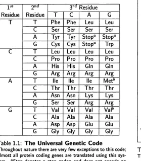
monly utilised in all biological systems (Table 1.2). With its alphabet of four letters one
nucleotide obviously does not code for one amino acid. Dinucleotides would only be able
to encode 16 amino acids, however trinucleotides could encode 64 amino acids. This
turns out to be the correct answer; the 64 possible trinucleotides are known as codons
and each has a particular meaning. The majority, 61 of them encode the 20 amino acids,
with varying degrees of redundancy. The remaining 3 are stop codons they mark out the
end of the protein coding sequences. The 64 possible codons make up the genetic code
are detailed in Table 1.1.
Redundancy
Redundancy is implicit in the genetic code, there are 4^ = 64 possible codons and only
20 (Table 1.2) amino acids. This simple calculation could infer two things: either most
of the codons do not code for anything or many of the amino acids are represented by
more than one codon. This is obviously the case, however it is important to note that
ist
Residue
2nd
Residue
3^^ Residue
T C A G
T T Phe Phe Leu Leu
C Ser Ser Ser Ser
A Tyr Tyr Stop" Stop" G Cys Cys Stop" Trp
C T Leu Leu Leu Leu
C Pro Pro Pro Pro
A His His Gin Gin
G Arg Arg Arg Arg
A T lie lie lie Met^
C Thr Thr Thr Thr
A Asn Asn Lys Lys
G Ser Ser Arg Arg
G T Val Val Val VaP
C Ala Ala Ala Ala
A Asp Asp Glu Glu
G Gly Gly Gly Gly
Table 1.1: The Universal Genetic Code
Throughout nature there are very few exceptions to this code; almost all protein coding genes are translated using this sys tem. "Stop denotes a stop codon and does not encode an amino acid. *’Both AUG and GUG may serve as initiation codons.
A Ala Alanine C Cys Cysteine D Asp Aspartic Acid E Glu Glutamic Acid F Phe Phenylalanine G Gly Glycine H His Histidine
1 lie Isoleucine K Lys Lysine L Leu Leucine M Met Methionine N Asn Asparagine P Pro Proline Q Gin Glutamine R Arg Arginine S Ser Serine T Thr Threonine V Val Valine W Trp Tryptophan
Y Tyr Tyrosine Table 1.2: Amino Acids
The 20 amino acids plus their respective one and three letter codes.
the distribution is far from even. As shown in Table 1.1 leucine, arginine and serine have
six different codons, cysteine and tyrosine have two whilst methionine and Tryptophan
have only one.
1.2
The Journey from Gene to Protein
The journey from a DNA sequence to a protein is not a direct one. There are many
intermediate stages, which make up the two major processes involved, transcription and
1.2.1
Transcription
Transcription generates a single stranded ribonucleic acid (RNA) molecule complemen
tary in sequence to the template DNA strand. There are three types of RNA that are
involved in protein synthesis: messenger RNA (mRNA), transfer RNA (tRNA) and ri
bosomal RNA (rRNA). Of these it is mRNA that encodes the protein sequence, whilst
tRNA and rRNA are active parts of the translation machinery. As a result it is mRNA I
will focus on here.
Transcription has many parallels with DNA replication. Firstly the DNA duplex is
partially unwound. This allows the binding of an RNA polymerase; this would be RNA
polymerase II in humans. This transcribes the DNA sequence into a complementary
strand of RNA. RNA is very similar to DNA except that the sugar that makes up the
backbone is ribose rather than deoxyribose. Secondly RNA has a slightly different base
composition to DNA with uracil replacing thymine. This single strand of RNA has a cap
of 5-methyl-cytosine and a poly-adenosine tail added to it to create the final messenger
RNA molecule. The mRNA strand must then be exported out of the nucleus before it
can undergo translation.
1.2.2
Translation
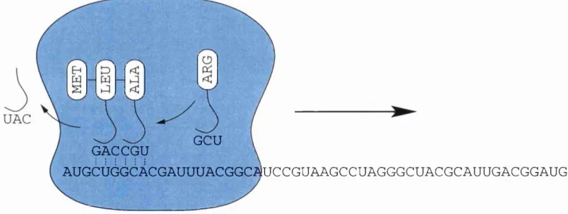
Once the mRNA is exported from the nucleus to the cytoplasm it will be bound by a
ribosome and translated in to protein (Figure 1.1). It is at this stage that the other RNA
types mentioned earlier play a role. The ribosome itself is a complex of both protein and
for each codon in the genetic code, these molecules can reversibly bind to their specific
amino acids. Each o f these molecules also contain an anti-codon for the amino acid
they carry, which is a trinucleotide w ith a complementary sequence to the codon. Via
this anti-codon they base pair to the mRNA bringing together the amino acid monomers
in the correct sequence order. As this occurs the ribosome catalyses the polymerisation
of these monomer units and the ir release by the tR N A . Once complete the protein is
released from the ribosome, after which it may undergo post-translational processing or
may be imm ediately exported to where it is required.
GCU GACCGU
AUGCUGGCÀCGAUUUACGGCAUC C GUAAGCCUAGGGCUACGCAUUGACGGAUG
Figure 1.1; Translation. The ribosome moves along the mRNA strand in the direction indicated catalysing the polymerisation of the amino acid monomers, which are assembled into the correct positions by the influence of the respective tRNA molecules.
1.3
Evolution
Living is a dangerous thing to do, during every minute o f every day our cells are under
attack, often from the products o f our own metabolism. There are many mechanisms
light, free radicals and a variety of chemicals can all damage and cause lesions on DNA.
These substances are mutagens i.e. they can induce mutations, in humans they would
often be referred to as carcinogens as many mutations can lead to the development
of cancer. Most of the time damage to a DNA strand is repaired without problems,
however occasionally a mistake in the repair mechanism will culminate in a mutation,
causing a change in the genetic sequence. DNA damage can also result in a mutation
during replication, when base pair mismatches and a host of other problems can occur.
Even in the absence of damage the process of replication can lead to mutation, for
example the DNA polymerase complex could slip leading to the duplication or deletion
of a short region of the DNA strand. If these mutations occur in germ cells then they
will be passed on to the progeny of the organism, becoming variants in the gene pool on
which evolution can then act.
For the purposes of this work we could define evolution as a change in the DNA
sequence of an organism that is passed onto it ’s progeny. This could be as simple as a
single base change in an organisms entire genome. However it is probably more true to
say that evolution has occurred when that change has become fixed in a population of
organisms, be it via selection or other means. A single change in a single organism really
only constitutes a new mutation or variant in the gene pool. There are a great many
factors that can determine whether that change will become fixed in the population. It
could be that the change is a synonymous one, i.e. it does not cause any change in the
protein sequence. This can be brought about if the mutation occurs in a non-coding
same amino acid. This is possible due to the degeneracy of the genetic code; changes in
the third base of many codons produce this result. If the mutation is synonymous then
the forces that will lead to it being fixed in a population are essentially random. If it's
frequency rises high enough by chance to become fixed then we can say this is a result
of genetic drift (King and Jukes, 1969). These types of changes can make two DNA
sequences that encode nearly identical protein sequences quite different at the nucleotide
level.
The second type of changes are non-synonymous ones. These are mutations that
cause a change in the protein sequence, for example a change in the second base of a
codon will nearly always have this effect. If the effect of this change is very mild causing
little or no change to the protein’s properties or activity then the self same random
effects can lead to loss or fixation, by a process known as neutral or nearly-neutral
evolution (Kimura, 1983). However if the mutation has a stronger effect e.g. conferring
an advantage of some kind to the carrier then natural selection may act to rapidly fix
the change in the population or if the effect is deleterious to remove it.
It is the cumulative effect of all these changes and many others that lead to the
differences observed between homologous sequences both within and between closely
related organisms. This is why when we wish to search for related sequences in sequence
1.4
Sequence Databases
With the advent of rapid DNA sequencing technology came the development of biological
sequence databases. Since their inception they have multiplied to create a large variety
of both specialised and general repositories. The largest and most well known is the
Genbank/EMBL/DDBJ database, containing virtually all the DNA and protein sequences
known to date. This is actually made up of three databases the Genbank database from
the NCBI, the EMBL database maintained at the EBI and the DNA Databank of Japan.
These three organisations share all data and submissions with each other to create a
‘universally accessible’ databank, for the remainder of this thesis I will refer to this
simply as the Genbank database.
There are several other commonly used databases. SWISS-PROT (Bairoch and
Apweiler, 2000) is a curated protein database with a minimum level of redundancy.
Its intention is to provide a high level of annotated information as well as the protein
sequence itself. This annotation can include details such as function, structure and
post-translational modifications. TrEMBL (Bairoch and Apweiler, 2000) is a supplement
to the SWISS-PROT database. It includes and attempts to automatically annotate all
the translations of Genbank nucleotide sequence entries not yet integrated in SWISS-
PROT. The protein data bank (PDB) (Berman et al., 2000) is a database of known
three-dimensional protein structures. Whilst this is not solely a sequence resource it is
extremely useful, structures can help us to judge when sequences are true homologues of
one another even when the sequences in question do not appear to share any significant
as it allows us to judge how well our database searching system is working by being
able to identify and quantify correct and incorrect hits. Derivatives of the PDB are
particularly useful for this purpose, specifically SCOP (Murzin et al., 1995) and GATH
(Orengo et al., 1997). These data sets seek to hierarchically classify sequences according
to their structure. SCOP is manually produced and focuses on reliability, only classifying
proteins together if there is significant evidence that they are related. CATH on the
other hand is largely automatically generated but still seeks to classify proteins and
their folds into homologous families. These classifications can then be used for grading
sequence searching systems or as a method of annotating new sequences (Park et al.,
1997; Brenner et al., 1998; Park et al., 1998; Müller et al., 1999; Salamov et al., 1999;
Pearl et al., 2000; Waliqvist et al., 2000).
In addition to these more established resources there are now a significant number
of organism specific databases, which have resulted from various genome sequencing
projects in addition to previous work. These include FlyBase (The FlyBase Consortium,
1999) for Drosophila and Worm Base (Stein et al., 2001) for C. elegans. Probably the
most well known to the world at large is the human genome sequencing project (Interna
tional Human Genome Sequencing Consortium, 2001), whilst the results of this are still
not fully complete, preliminary results are available in various forms. The impact of these
various genome sequencing projects upon all the databases has been massive. Already
growing at an alarming rate, the number of sequences being deposited has taken yet
another leap over the past two years. As these databases get larger so do the problems
Whilst these large centralised data resources do have great potential use for scientists,
they do also present a problem. The non-redundant Genbank database has 750,000
sequences; in this amount of data the problem is to locate the ones you are interested in.
Ideally each sequences would be catalogued by organism, position in the genome, name
of gene, function of protein and we could then simply search for and find our sequence
of interest. Unfortunately things are not as simple as this. Whilst this information is
often put into the sequence entries, it is not always available. Many genes have been
sequenced without knowing what the protein they encode. This type of data is routinely
produced by the various genome sequencing projects, in fact they produce large amounts
of sequence data where it is not even known where the genes lie yet alone what they
encode.
Furthermore this approach is fine if you have a simple query like: Find all globin gene
sequences from the mouse Mus musculus. Effective systems to do this Job already exist
e.g. the Entrez interface (http://www.ncbi.nlm.nih.gov/Entrez/) at the NCBI
website. However what if we have a DNA or protein sequence and we want to find any
similar sequences in the database. For example we might have a fragment of a gene and
wish to find out if the entire length has already been sequenced. Or we may wish to
identify homologues in different species, or other members of the same family of genes.
1.5
Sequence Comparison & Database Searching
The need to be able to compare sequences with one and other has always been apparent.
Initially a simple question like how do two related sequences line up against each other
i.e. which residues are conserved could be answered by aligning the two sequences by
eye. However this is a time consuming process and requires a certain degree of expert
knowledge. What was needed was some method of automating this process.
1.5.1 Sequence Alignment
Sequence alignment is a far from trivial process. When aligning by eye an expert can
take many factors into account including the biological properties and the prevalence of
the various amino acids and also perhaps their relationship to the surrounding sequence
e.g. taking into account knowledge of the proteins structure. Also most importantly it
has to be decided when and where to introduce gaps in the sequences to fully align them.
It is therefore not as simple a task as many might think for a computer to automate.
When attempting to align sequences it is important to bear in mind which amino acids
you consider similar and which dissimilar. The simplest approach would be to consider
only identities, for example an amino acid scoring matrix based on identities only would
give a score of 1 to an identical match and zero otherwise. Whilst this system would
work for closely related proteins with very high sequence identities, it would be useless
for more divergent ones. A relatively simple way around this problem is to consider which
amino acids have similar physical and chemical properties for example we could consider
dissimilar because of its acidic group. Qualitatively this method makes a lot of sense
however it is difficult to quantify, for example how much more similar would we consider
serine to threonine as opposed to tyrosine and vice versa. Another simple solution would
be to use the genetic code (Table 1.1) itself to judge the relationships, it is possible to
calculate the minimum number of base changes required to change any amino acid into
any other amino acid. It is also possible to draw inference on how much we can read
in to amino acid identities (when an amino acid matches itself). Methionine only has
one codon whereas serine has six; should a serine-serine match only score a sixth of a
methionine-methionine one, the genetic code would draw you to think so. As attractive
as this concept of scoring may be it is far from prefect. It probably does give an indication
of how often specific amino acid changes occur. However it does not indicate how often
these changes become fixed and it does not take into account the effects of evolution,
specifically those of selection. Therefore a way of judging how frequently one amino acid
changes to another in real sequences is needed.
The first attempt to do this was the PAM (Point Accepted Mutations) matrices
(Dayhoff et al., 1978). This series of matrices was based upon alignments of very
closely related sequences sharing at least 85% identity. The amino acid substitutions
observed in these alignments were recorded and converted to mutational probabilities
according to 1% accepted mutations - one amino acid changed in 100. This matrix was
then scaled by self-multiplication to produce the other matrices of the set which are
applicable to more distantly related sequences e.g. PAM250 log odds matrix represents
have proven to be remarkably effective. The work has been repeated with newer larger
datasets (Jones et al., 1992) but the original set are still widely used. In fact it is only in
the last decade that another popular substitution matrix set has arisen. The BLOSUM
(Henikoff and Henikoff, 1992) matrices were derived from approximately 2000 blocks
of aligned sequence segments from more than 500 groups of related proteins. Whilst
both the BLOSUM and PAM matrices have proven very effective for sequence alignment
and database searching there is a certain amount of empirical evidence (Henikoff and
Henikoff, 1992; Henikoff and Henikoff, 1993) pointing to the BLOSUM set being slightly
more reliable.
These matrices provide a reliable method of judging the probability that one amino
acid will be substituted for another over evolutionary time. The next dilemma is how to
use this information to compute the best alignment of two protein sequences.
Dynamic programming
The solution to this problem is most generally credited to Needleman & Wunsch (Needle-
man and Wunsch, 1970). The procedure they introduced is now commonly known as
dynamic programming. The dynamic programming algorithm operates in two steps.
Taking two sequences A and B firstly a search matrix is constructed of dimensions mn
with m being the length of sequence A and n of sequence B. The matrix is filled from
the top left to the bottom right corner, each cell [z, j ] receives the score of the exchange
value of residue A% and B^ plus the maximum score of row z — 1 and column j — 1
minus any incurred gap penalties. Cell [z,j] therefore contains the maximum score for
simply written as:
— l , j — 1]
maxi<a;<i(5[i — x , j — 1] — P (x — 1)) (^-^)
maxi<y<j(5[i — \ , j — y\ — P {y — 1))
Where S[ i , j ] is the score of the best alignment of sequences A and B up to residues i and
j respectively. The s [ i , j ] term refers to the exchange value of the residues associated
with cell [ i j j ] . The Max term denotes the maximum score of the three equations detailed
in the brackets. The first term would be the maximum in the cases where no gap had to
be inserted at this position in the alignment. The second would be true if a gap had to
be inserted in sequence B for residues i and j to be aligned. The third term obviously
corresponds to a gap insertion in sequence A. P { x — 1) is a non-negative penalty value
for a gap of length x — 1 with l < x < i denoting the range of values x could possibly take.
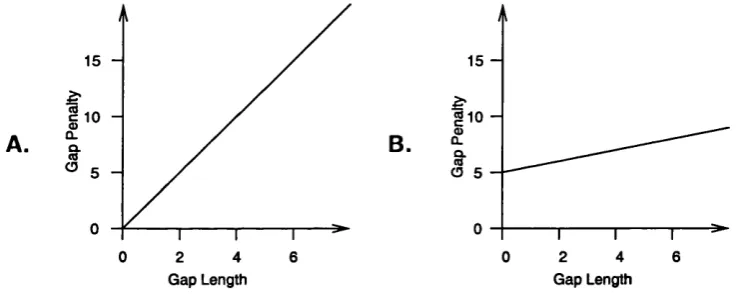
In its original implementation (Needleman and Wunsch, 1970) this gap penalty was
defined as a fixed value for the inclusion of a gap of any length. This idea was soon
replaced by the concept of length-proportional gap costs (Sellers, 1974) where a gap of
length X would have the penalty P( x) = Gx, where G is the cost of a gap of length 1.
However over the years it was noticed that the highest scoring alignments produced using
length-proportional gap costs often contained a large number of short gaps. Such a high
number of short insertions or deletions was not thought to be very plausible. Because
a single mutation may result in the insertion or deletion of a large number of residues
not cost sizably more than a short one. Affine gap costs use two gap penalties, Go the
penalty for opening a gap and Ge the penalty for extending a gap giving the formula
P{x) = Go + GeX. This scheme is the predominant one employed by modern alignment
packages, typically Go will be a order of magnitude larger than Ge therefore making it
difficult enough to open a gap but relatively easy to extend it where necessary. The
difference between length-dependent and affine gap costs can be seen in Figure 1.2.
A.
15
0
0 2 4 6
B
15
-9 1 0
-0 2 4 6 Gap Length Gap Length
Figure 1.2: A comparison of length dependent and affine gap costs A . length dependent gap penalty o f 5 per unit length. B. Affine gap score; gap opening penalty o f 10, gap extension penalty o f 1 per unit length.
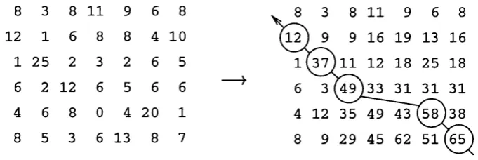
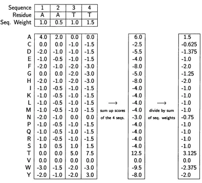
The second stage of the dynamic programming algorithm is the traceback step. It
is at this point that the actual optimal or highest scoring alignment is reconstructed.
Starting from the cell with the highest alignment score which will lie in the final row
or in on the final column. The path is traced back following successively lower scores,
each time selecting the highest scoring cell from the previous column or row from the
present position. This continues until both the sequences are fully aligned i.e. until the
traceback reaches the first row or column. This procedure is graphically illustrated in
8 3 8 11 9 6 8 8 3 8 11 9 6 8
12 1 6 8 8 4 10 1 9 9 16 19 13 16
1 25 2 3 2 6 5 11 111 12 18 25 18
6 2 12 6 5 6 6 ~ 6 3 |33 31 31 31
4 6 8 0 4 20 1 4 12 35 49 (S8 )38
8 5 3 6 13 8 7 8 9 29 45 62 51
Figure 1.3: The Dynamic Programming Algorithm. T h e initial alignm ent m atrix is shown on the left, the values are then summed (taking into account any gaps) to produce the m atrix on the right. T h e final alignment is then realised by the traceback step starting from the highest scoring cell.
The dynamic programming algorithm will always find the optimal alignment between
two sequences for a given scoring scheme. This is fine when the sequences share a certain
degree of similarity e.g. 40% sequence identity. When the sequences are much more
divergent perhaps only sharing 25% sequence identity a global alignment such as this,
where the full lengths of both sequences are aligned, may be far less useful and more
worryingly it may be completely wrong. If the two sequences share only short sections
of homology then an optimal global alignment may miss these segments either in the
noise generated by the divergent regions or the gap penalties may prevent these conserved
segments from being successfully joined. Just because it is possible to align two unrelated
sequences it does not mean that the sequences share any significant degree of similarity.
Two random sequences will share approximately 20% sequence identity when aligned
globally. In cases where the sequences are distantly related we are often more interested
Local Alignm ent
In addition to the problems already discussed many proteins are modular in structure,
made up of discrete units known as domains. These domains which are mainly defined
in a structural context can be present in a wide variety of proteins, although not always
in the same order. In such examples a global alignment of two sequences would be
meaningless. Consider a case where two proteins share a domain, in sequence A the
domain makes up the final quarter of the sequence and in sequence B it makes up the
first quarter. In most cases a global alignment method would not pay attention to an
alignment of the first section of one sequence to the last of another. In fact in many
programs to save time this section of the alignment matrix is not even calculated as a
match is such a position is considered unlikely or wrong. There are also other possibilities
that can limit the effectiveness of global alignment methods, for example the occurrence
of internal sequence repeats.
In these circumstances the best strategy is to undertake a local (Smith and Waterman,
1981) as opposed to global alignment. A good way to describe the local alignment
technique is that the most similar regions of two sequences are selected and aligned,
paying no attention to dissimilar regions or linear ordering. The method is essentially the
same as the global alignment algorithm, with a few additional conditions and stages. A
dynamic programming algorithm is implemented but in this case the amino acid exchange
values used must include negative values. Any score in the search matrix that would
be negative is set as zero. The algorithm relies on dissimilar subsequences producing
zero. Equation 1.1 thus becomes:
S [ i J ] = s[i,j] + Max < (1.2)
— 1]
maxi<a;<i(5[i — x , j — 1] — P (x — 1))
maxi<y<j(5[i — 1, j — y] — P{y — \))
0
The consequence of these changes is that the highest alignment or more correctly sub
alignment score no longer has to be in the final row or column but can appear anywhere
in the matrix. Once the highest scoring segment has been traced back it is but a simple
procedure to find the next highest scoring sub-alignment. To do this the second highest
scoring cell in the scoring matrix is located and traced back. However when this is done
you must be careful to exclude the cells that make up the first sub-alignment, otherwise
you will merely traceback along the same route. Following this procedure it is possible
to locate all of the top scoring non-intersecting sub-alignments of the two sequences.
The point at which the sub-alignments cease to be top scoring is obviously user defined.
Multiple Alignment
The mechanisms covered so far relate to pairwise alignments, i.e. the comparison and
search for similarity between a pair of sequences. Whilst the number of available se
quences was small this was an adequate solution. However as the number of sequences
has grown and specifically when large sets of homologous sequences are available we
once. In theory a multiple alignment should not be difficult to construct or calculate,
however the speed of the dynamic programming algorithm is dependent on the prod
uct of the lengths of the sequences being aligned. In a pairwise alignment this is just
mn the size of the search matrix, for three sequences we would have to construct a
three-dimensional search matrix, for four it would be four-dimensional and so on. The
number of calculations quickly become prohibitive. Imagine trying to simultaneously
align four sequences each two-hundred amino acids in length, this would give a search
matrix of size 200^ = 1.6 x 10® this is a 40000 times larger computation space than a
pairwise comparison of the same length. With the computation time being proportional
to this it is easy to see that even with modern computers the time and resources needed
to undertake such calculations is prohibitive. Methods have been developed that allow
the multiple alignment of up to 10 sequences of a certain length (Lipman et al., 1989;
Johnson and Doolittle, 1986). Although they work in different ways these algorithms
make the problem tractable by reducing the search space effectively ruling out possible
but unlikely alignment results. Being able to align ten sequences is not enough for most
biologists, many of the sequence families in the databases have had a large number of
their members sequenced. A simple search shows that well over 500 globins have been
sequenced. Trying to complete a true multiple alignment of this number of sequences is
frankly ridiculous.
The unfeasibility of a truly simultaneous multiple alignment algorithm that can work
with large numbers of sequences has led to the development of various heuristic ap
strategy (Hogeweg and Hesper, 1984). The basis of this strategy is to align the closest
sequences first and successively adding in the more distant ones until all the sequences
are joined in a final multiple alignment. In essence this method reduces the multiple
alignment to a serial sequence of pairwise alignments.
A good example of this method is the CLUSTAL alignment programs (Higgins and
Sharp, 1988). This original program was designed specifically to run on desktop com
puters and thus had to be not too computationally demanding. The program firstly
uses a fast pairwise alignment step to evaluate all the possible pairs; it then uses this
information to construct a guide tree using the un-weighted pair group mean arith
metic (UPGMA) method (Sneath and Sokal, 1973). The sequences are then aligned
following the branching order of the guide tree. When groups of sequences came to be
aligned the original implementation used consensus sequences to represent the aligned
subgroups. The CLUSTAL program has been developed and refined over the years:
CLUSTAL V (Higgins et al., 1992) implemented a more efficient dynamic programming
routine; CLUSTAL W (Thompson et al., 1994) made use of the Neighbour-Joining (NJ)
algorithm (Saitou and Nei, 1987) to construct the guide tree and rather than consen
sus sequences, sequence blocks were represented using profiles. The success and speed
of this method has made CLUSTAL W and CLUSTALX (Thompson et al., 1997) its
graphical counterpart probably the most widely used alignment package.
Other techniques have of course been developed, some such as MULTAL (Taylor,
1988) are variants of the progressive alignment strategy. More recently more novel
1998) makes use of a genetic algorithm to align the sequences, T-Coffee (Notredame
et al., 2000) attempts to integrate information from various sources including local
and global alignment information to construct a multiple alignment. Many of these new
techniques have much to offer, however none of them match the speed of the progressive
alignment approach, which will undoubtedly remain a favourite for some years to come.
1.5.2
Database Searching
Both pairwise and multiple sequence alignment have developed into commonly used tools.
These tools are extremely useful for bioinformatics and bench biologists alike. They allow
us to compare two or more sequences together and to putatively infer structure, function
and evolutionary history. But given a sequence we are interested in how can we search
the database for similar sequences. One solution would be to carry out global pairwise
alignments of our query sequence against every other sequence in the database, it would
then be possible select all the sequences with the highest alignment scores as probable
homologues of our query. Unfortunately this is not really a feasible option. Firstly
there are at present approximately 750,000 sequences in the non-redundant Gen bank
database. Doing the better part of a million alignments every time you want to search
the database would be a very time intensive method. Secondly a global alignment would
not be the best method for assessing similarity, as I have already mentioned global
alignment methods can make mistakes when the sequences are distantly homologous,
especially when only segments of the sequences share any degree of homology. In effect
what we need to do is carry out a local alignment comparison of our query sequence to
Sm ith-W aterm an search
The idea of a Smith-Waterman (Smith and Waterman, 1981) based search is a very
attractive one. It should theoretically allow the accurate recognition of even quite re
mote sequences that share only short regions of homology. The same problem still
exists, carrying out such a large number of pairwise local alignments is generally time
prohibitive. This has not however prevented the development of such methods, of these
the SSEARCH program (Pearson and Lipman, 1988) is probably the most well known.
Because this approach is so exhaustive it has been frequently used as a yardstick to com
pare new approaches to database searching (Shpaer et al., 1996; Agarwal and States,
1998; Brenner et al., 1998). Attempts to accelerate this procedure have frequently relied
on the use of expensive parallel computers. These are generally refered to as hardware
implementations of Smith-Waterman, as well as being much faster have proven to be just
as effective as their software counterparts at finding homologues (Shpaer et al., 1996).
However the high cost of this machinery has meant that they are not in widespread
use. Recent work has made use of special instruction sets present in common desktop
computers to accelerate the search procedure (Rognes and Seeberg, 2000). This type of
method holds a lot of promise, however the speed of searching still does not approach
the heuristic methods that have been developed over the last decade.
Heuristic algorithms
Heuristic alignment algorithms were intentionally devised with database searching in
database for similarities to a given query sequence. There are two families of heuristic
programs in general use, the FASTA (Pearson and Lipman, 1988; Pearson, 1990) and
BLAST (Altschul et al., 1990) programs.
The first step in the FASTA program is to search for identical ‘words’ of a defined
length (known as /f-tuples) in both the query and target sequences. Generally for proteins
a word length of two {ktup = 2) is sufficient for most searches, it combines good
accuracy with high speed. A higher value increases the speed but at the risk of increasing
inaccuracy. These /r-tuples are then used to identify the ten most interesting diagonal
regions in the alignment matrix. These regions are then re-scored using an amino acid
substitution matrix, thus taking amino acid similarities into account as well as identities.
Only regions with a score above a cutoff value are considered further. A gapped alignment
score is estimated by joining together compatible regions using a Joining penalty. FASTA
also computes an optimal local alignment restricted to a band centred on the highest
scoring region. Finally these scores are used to estimate the statistical significance of
the matches.
The BLAST programs work in a similar way. However it is important to differentiate
between the two BLAST programs that are commonly used for protein-protein sequence
searches. BLASTP (Altschul et al., 1990) is the original program developed for searching
protein sequence databases and is still in common use. BLASTPGP (Altschul et al.,
1997) is a more advanced version and works in a significantly different manner. In the
first step BLASTP uses words of length w. Unlike FASTA, BLAST allows the words
match at score greater than T when scored using the amino acid substitution matrix.
By default BLASTP uses the parameter settings w = 3 and T = 11. In the second
step BLASTP extends the initial words in both directions using the substitution matrix
to form high-scoring segment pairs (HSPs). The extension is stopped when potential
score of the extending segment drops below the the maximum score of the HSP within
the segment. This version of BLAST does not consider gapped alignments at all but
uses sum-statistics (Karlin and Altschul, 1990; Karlin and Altschul, 1993) to compute
the significance of the matches from the highest scoring HSPs.
The BLASTPGP algorithm shares many similarities with the original BLASTP algo
rithm, however several key improvements have been made and to fully accommodate
these the procedure has been changed somewhat. As before the program looks for all
the words of length w scoring above T. However to reduce the number of words that are
extended (in the original implementation this accounted for approximately 90% or more
of the computation time) the refined algorithm looks for two non-overlapping words on
the same diagonal of the scoring matrix, no further apart than A residues; for w = 3 and
T = 11 it is recommended that A = 40. If two words are matched within the required
distance then an ungapped extension of the second word is triggered. If the HSP gen
erated has a normalised score above a cutoff then a gapped extension is triggered. This
Smith-Waterman like extension requires 500 times the computation time of that of an
ungapped one, however because extensions are triggered so much less frequently than
in the BLASTP program one gapped extension will only be triggered for upto 4000 un
extensions are significantly reduced, the total time spent on the extension stage is cut by
a factor of two. The significance of the gapped alignments is then evaluated (Altschul
and Gish, 1996) before the results are reported.
Significance of matches
There one important problem that I have already alluded to that remains when under
taking a database search. How do you evaluate when a match is a true hit i.e. at what
alignment score is a match no longer considered a true homolog. This is not a clean cut
problem, it is not possible to define an arbitrary alignment score cut off value, longer
sequences have a higher probability of producing a higher alignment score by chance
alone. This problem has been dealt with by several methods but almost ubiquitously all
search engines now evaluate the statistical confidence of their hits. Put most simply this
is the probability that a hit of score score x would occur by chance.
If we assumed that the scores obtained by random sequences in database searches
followed a normal distribution it would be a simple matter to calculate the probabilities,
using the mean and standard deviation of all the scores it is a simple matter to assess
the probability of achieving a score greater than x. However the scores do not follow
a normal distribution and such a calculation would lead to gross errors in the estimates
of confidence. The distribution of scores for an ungapped local alignment of random
sequences has been shown to follow an extreme value distribution (Karlin and Altschul,
1990). For this to be true certain conditions have to be met, uppermost of these is that
the expected score 3 pah^ of randomly chosen residues is negative.
This makes good sense, if the probability was positive then local matches would tend to
extend to the full sequence length. Luckily scores based on likelihood ratios such as the
PAM and BLOSUM matrices always satisfy this condition. As long as this condition is
met and at least one of the scores has a positive value it is possible to calculate one of
the parameters of the extreme value distribution. A is the unique positive solution for x
in Equation 1.3.
20
E = 1 (1.3)
i , j = l
The second parameter that is important to our calculations is K , this is a constant which
is defined by a geometrically convergent series, which is dependent on the scoring scheme
i.e. the values of pi, pj and The formula to calculate K is explicitly defined but
due to its complexity I have decided not to reproduce it here; it is well documented in
the appendix of Karlin and Altschul (1990). Using these two parameters it is possible to
calculate the probability of achieving a score S greater than or equal to x the observed
score.
P{S > x) = 1 — exp{—Kmne~^^) (1.4)
The two parameters that have not been discussed yet, m and n, are the lengths of
the query and target sequences respectively. For a database search the target sequence
can be thought of as the database as a whole therefore n would be the length of the
database in residues. It is on this general basis that all the statistical evaluations of
sequence hits are based. Of course this formula only applies to ungapped alignments,
newer implementation of both BLAST and FASTA produce gapped local alignments as
rather than ungapped ones. An extension of this theory which is known as sum statistics
(Altschul and Gish, 1996) allows the assessment of a set of top scoring local alignments
rather than just the optimal segment via the sum of their scores. From this it has been
shown empirically that the results from gapped local alignments seem to fit this function.
However because the gap penalties alter the scoring scheme the values of A and K for
gapped and ungapped alignments are different. For gapped alignments these parameters
cannot be estimated directly and instead have been estimated by fitting Equation 1.4 to
scores from simulations. When gapped alignments are used a better result is obtained
when the sequence lengths are corrected for edge effects. Because a subalignment does
not exist at a single point it cannot start near the end of either sequence or it will run out
of space before it can reach an optimal score. As a result to correct for this edge effect
it is advisable to estimate the effective length of the sequences. Equation 1.5 shows how
to calculate the effective length m! for sequence m, with the n' calculation following the
same format. H is the relative entropy of the scoring system (Altschul, 1991; Altschul
and Gish, 1996).
, \ n K m n
m « m —— (1.5)
Rather than P-values the new versions of BLAST utilise E-values (Altschul et al.,
1997; Schaffer et al., 2001). These are the expected number of subalignments of random
The significance testing methods utilised by the FASTA suite of programs are also based
on the extreme distribution theory. However the implementation of this is somewhat
different (Pearson, 1998). Rather than using pre-computed values of A and K , the
distribution is itself calculated using all the similarity scores produced during the database
search. The mean (/i) and standard deviation (a) are related to K m n and A and are
easy to calculate from these scores. This should mean that the correct distribution
parameters are calculated each time, regardless of the scoring system or gap penalties
used. However, the estimation is only accurate if all the sequences are unrelated e.g. if
random sequences are used. However in a real search some sequences will be related,
indeed these are the very sequences we are trying to locate, the homologues of our query
sequence. When the dataset includes these related sequences this method of estimating
the significance breaks down the effective values of K and A that are implied by the
distribution will be incorrect and will mean that the significance values reported will be
incorrect, true hits would be ignored as false. To overcome this problem the authors
of FASTA implemented a filtering system with the intent of removing any scores that
might be from related sequences so that a correct estimate could be made.
z = (1.7)
Before the significance of a hit is calculated, its score is converted in to a z-va lue as shown
in Equation 1.7. This z-va lue is then converted to a P-value using the extreme value
can be found in Pearson (1998).
P { Z > z) = 1 — exp(—e (1.8)
The filtering method used splits all of the scores up into separate 'bins' according to
the lengths of the sequences, the means and standard distribution of each of these bins
is calculated and a simple linear regression line is calculated for the means of the bins.
The z-va lues of all the scores are then calculated with the mean of each bin being taken
from the regression line. Any scores with z-va lues <-3.0 or >5.0 are excluded before
the procedure is repeated for a second time. Once complete are the remaining scores
are used to estimate the extreme value distribution used to calculate the final P-values.
Advanced Search Schemes
As good as these heuristic programs have become and as accurate as the full Smith-
Waterman search is, these methodologies still have limits to their success in finding
homologues. The main limiting factor is that these are all pairwise approaches, they
compare one query sequence to each sequence in the database. What they do not
and can not do is take into account the information contained in any homologues that
have already been identified to the query sequence i.e. the searches do not incorporate
information on the protein family of the query sequence. The idea of doing such a thing
is so that homologues that are much more remote can be isolated, which when compared
to the query sequence alone show no definite homology.
method (Park et al., 1997). This approach makes use of intermediate sequences to
find remote homologues, for example if sequences one and two match each other with
a high score and sequences two and three match with a high score, we can infer that
one and three are homologous even though when compared directly they have a low
score of similarity. This method and other similar ones (transitive sequence searching
(Neuwald et al., 1997), systematic re-searching (Krause and Vingron, 1998) and multiple
intermediate sequence searching (Salamov et al., 1999)) have proven to be very effective
at recognising more remote homologues than the simple pairwise systems (Gerstein,
1998; Park et al., 1998).
Whilst ISS and related methods are simple and effective they are largely just a more
complex way of carrying out a pairwise search. However methods have been developed
that can use more than one sequence at once to search a database. These are the profile
search methods, of these the most predominant is PSi-BLAST (Altschul et al., 1997;
Schaffer et al., 2001). As it's name indicates PSI-BLAST is a member of the BLAST
suite of programs available from the NCBI. It works in almost exactly the same way as
BLASTPGP, in fact a single iteration of PSI-BLAST is Just BLASTPGP. However the
program is designed to iterate and sequences found in the first round are used to help find
more distant homologues in the second round and so on. PSI-BLAST is not a true profile
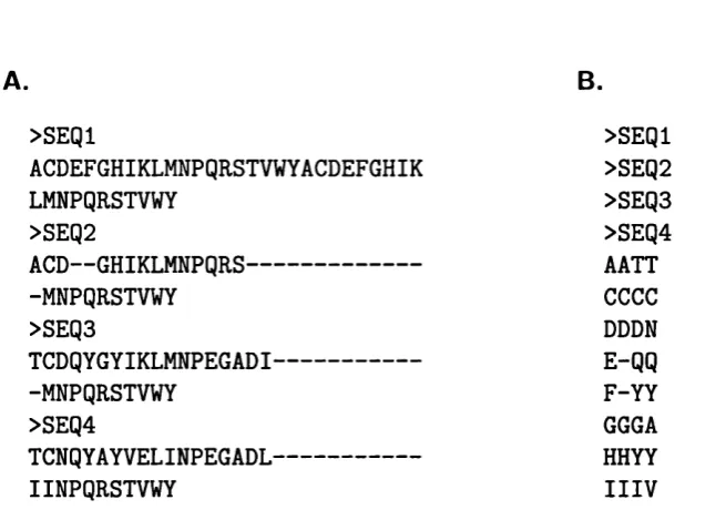
based database search engine. What it does is use the results of previous rounds or a user
defined alignment to produce a position specific scoring matrix (PSSM) for the query
sequence. The PSSM is a very powerful tool rather than relying on a substitution matrix
define which substitutions are most likely at each position in the query sequence on the
basis of the hits already found. To form the PSSM PSI-BLAST uses a pseudo-multiple
alignment of all the hits above a set threshold e.g. default is an E-value of 0.01. I refer
to this as a pseudo-alignment because the hits are stacked on top of the original query
sequence and no attempt is made at a full alignment, which would involve aligning all
the hits to one another as well. Identical sequences are excluded from the alignment as
are any sections that would involve the insertion of a gap in the query sequence, the
aim of this is to make the PSSM the same length as the query sequence. One of the
main reasons for not conducting a full multiple alignment is to keep the computation
time to a minimum. In comparison to a database search a full multiple alignment is
much more time intensive. The PSSM is then constructed from the pseudo-alignment
using a modified version of the Henikoff and Henikoff weighting scheme (Henikoff and
Henikoff, 1994; Altschul et al., 1997). PSI-BLAST continues iterating until the search
has converged, finding no new hits over the set threshold, or until it reaches the maximum
number of iterations set by the user. The power and success of this method has been
demonstrated in several different benchmarks (Park et al., 1998; Müller et al., 1999).
A somewhat different approach is taken by the QUEST program (Taylor, 1998; Taylor
and Brown, 1999). Unlike PSI-BLAST, QUEST uses an independent multiple alignment
program MULTAL (Taylor, 1987; Taylor, 1988) to align the sequences between iterations,
thereby hopefully improving the quality of the profile fed into the next stage. QUEST
also incorporates two screening steps between iterations. The first removes sequences
any incorrect sequences so that the profile does not become 'polluted'. The second
screening step is similar to one of the PSI-BLAST steps simply removing any sequences
that are too similar thus preventing them becoming overrepresented and hijacking the
profile. The search phase itself is not that dissimilar to the BLAST methods, the main
difference comes from the automatic optimisation of several parameters on the fly. These
parameters are the score cutoffs that will ultimately determine the speed, accuracy and
success of the program. The idea of this automatic control of these parameters is to
allow a relative novice to use the QUEST program and achieve very successful results
without needing any specialist knowledge on judging alignment quality. The success of
this approach has been evaluated and has been found to be quite effective (Taylor, 1998;
Taylor and Brown, 1999).
A different approach is again used by hidden Markov model (HMM) based search
systems. These approaches actually follow the profile based systems quite closely, but
rather than a profile an HMM is used to model the sequence information. HMMs are
a class of probabilistic models that are particularly applicable to linear sequences, such
as biological sequence information. Much of their appeal derives from the strong math
ematical and statistical theory that is their cornerstone, as opposed to the sometimes
ad-hoc system used in generating profiles. There is not space here to explain the theory
behind hidden Markov models, nor could I do it justice. There are however several good
reviews of HMMs and their application in biological sequence analysis (Durbin et al.,
1998; Eddy, 1998). Good examples of HMM based approaches are SAM-T98 (Karplus
et al., 1998) and HMMER (http://hmmer.wustl.edu), which are proving to be ef