Efficient Generation of Power In Medium Voltage Direct Current Systems: Variable Speed Operation and Rectifier Considerations

(1)

University of South Carolina

Scholar Commons

Theses and Dissertations

1-1-2013

The Effects of Mean Sea Level and Tidal Amplitude

On Ground Water Discharge and Pore-Water

Salinity Distribution Along A Forest/Marsh

Boundary, North Inlet, SC

John Bradley Peurifoy

University of South Carolina - Columbia

Follow this and additional works at:https://scholarcommons.sc.edu/etd Part of theEarth Sciences Commons

This Open Access Thesis is brought to you by Scholar Commons. It has been accepted for inclusion in Theses and Dissertations by an authorized administrator of Scholar Commons. For more information, please [email protected].

Recommended Citation

(2)

THE EFFECTS OF MEAN SEA LEVEL AND TIDAL AMPLITUDE ON GROUND WATER

DISCHARGE AND PORE-WATER SALINITY DISTRIBUTION ALONG A FOREST/MARSH

BOUNDARY,NORTH INLET,SC

by

John B. Peurifoy

Bachelor of Science University of South Carolina, 2007

Submitted in Partial Fulfillment of the Requirements

For the Degree of Master of Science in

Geological Sciences

College of Arts and Sciences

University of South Carolina

2013

Accepted by:

Alicia M. Wilson, Director of Thesis

Scott M. White, Reader

James Morris, Reader

(3)

ii

(4)

iii

DEDICATION

This thesis and graduate degree are dedicated to my daughter Madelyn Grae

(5)

iv

ACKNOWLEDGEMENTS

I would like to sincerely thank Alicia Wilson for allowing me to complete my

Master’s degree under her guidance. Thank you for being patient with me throughout this

process and for imparting your knowledge of groundwater processes and numerical

modeling to me. You have been and will continue to be an exceptional teacher, advisor

and friend. Many thanks are also due to my lab mates Andrea Hughes and Tyler Evans.

Both of you have provided me with valuable insights into my research and countless

hours of enjoyable conversation. It has been a pleasure getting to know you both, and I

(6)

v

ABSTRACT

Advective groundwater flow in salt marshes is an important mechanism through

which nutrients are exported to adjacent coastal waters. Groundwater flow also influences

the distribution of pore-water salinity in the subsurface marsh, which affects botanical

zonation, nutrient transport, and primary productivity. Recent idealized marsh island

simulations have suggested that increases in tidal amplitude result in increased

groundwater discharge, and that the elevation of MWL relative to the marsh platform is

inversely related to groundwater discharge. These simulations were only representative of

marsh islands (as opposed to forest-marsh boundaries) and considered simple, idealized

tides only. The results were not confirmed in a real field setting. This study utilized tidal

records and hydraulic head records to calculate and compare groundwater discharge

along two marsh environments: 1) a fringing marsh boundary that was influenced by a

large freshwater lens and 2) a marsh island with a much smaller freshwater lens.

Electrical resistivity surveys were conducted to image seasonal pore-water salinity

distribution. The discharge trends were then correlated to trends in MWL and subsurface

salinity. Our results indicated that discharge from the marsh to Crabhaul Creek was

dependent on the position of MWL. Observations showed increases in groundwater

(7)

vi

high marsh root zone, the occurrence and magnitude of discharge or recharge depended

on precipitation, tidal amplitude and MWL. The electrical resistivity surveys depicted

two distinct salinity zones, neither of which displayed any correlation to MWL or tidal

amplitude. The first was a shallow tidally-influenced zone containing saline to brackish

pore-water, and the second was a deeper freshwater flow zone. These results

demonstrated the importance of MWL and tidal amplitude on discharge and hence

nutrient export from salt marshes. It can be inferred that long-term sea level rise (at a rate

that exceeds sediment accretion) will significantly decrease nutrient export from salt

(8)

vii

TABLE OF CONTENTS

DEDICATION ... iii

ACKNOWLEDGEMENTS ... iv

ABSTRACT ...v

LIST OF TABLES ... viii

LIST OF FIGURES ... ix

LIST OF ABBREVIATIONS ... xi

CHAPTER 1 INTRODUCTION ...1

CHAPTER 2 SITE LOCATION ...5

CHAPTER 3 METHODOLOGY ...9

CHAPTER 4 RESULTS ...15

CHAPTER 5 DISCUSSION ...31

CHAPTER 6 CONCLUSION ...38

REFERENCES ...41

APPENDIX A ELECTRICAL RESISTIVITY PARAMETERS ...43

(9)

viii

LIST OF TABLES

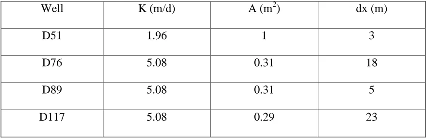
Table 3.1 Volumetric flux calculation parameters ...10

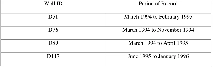
Table 3.2 Hydraulic head data records for wells located along Transect D ...11

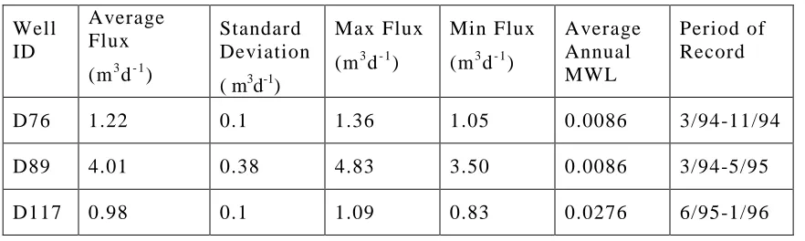
Table 4.1 Volumetric flux statistics for periods of record ...16

Table 4.2 Statistical analysis of resistivity and salinity results ...27

(10)

ix

LIST OF FIGURES

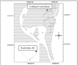
Figure 2.1 Geographic locations of North Inlet, SC and the Crabhaul

Creek Basin ...5

Figure 2.2 Cross-section of Transect D showing well nest locations,

geology, and groundwater flow directions...8

Figure 4.1 Volumetric flux at D76 (dots) and MWL (solid line)

between March 1994 and November 1994 ... 17

between March 1994 and April 1995...18

between June 1995 and April 1996 ...19

between March 1994 and April 1995...21

Figure 4.5 a) Hydraulic head record of D51 at 0.6 and 3.6 meters bgs b) Precipitation record for North Inlet c) 15-day running

average of MWL ...22

Figure 4.6 Total discharge and total recharge response to tidal amplitude

in D89 (January 1995) ... 24

Figure 4.7 Elevation of high tide versus total recharge in D89 (April

1994 to April 1995) ... 25

Figure 4.8 Electrical resistivity inversions from June 30, 2012, August 1, 2012, January 11, 2013, and May 22, 2013. Dashed lines represent

(11)

x

Figure 4.9 Percent difference plots (%) between a) June and August 2012 b) August 2012 and January 2013 and c) January and

May 2013. ... 29

Figure 4.10 Salinity and resistivity plotted against distance along Transect D at a depth of 3 meters for a) June 30, 2012, b) August 1, 2012,

c) January 11, 2013 and d) May 22, 2013 ... 30

Figure 5.1 Electrical resistivity surveys a) June 30, 2012, b) August 1, 2012, c) January 11, 2013, and d) May 22, 2013 and e) 29-day running

average of MWL position ...37

Figure 5.2 Daily precipitation totals for a) June 1 to 30, 2012 b) July 2 to August 1, 2012 c) December 12 to 27, 2012 d) April 23 to

(12)

xi

LIST OF ABBREVIATIONS

AGI ... Advanced Geosciences Incorporated

bgs ... Below Ground Surface

ET ... Evapotranspiration

IP ... Induced Polarization

LTER... Long-Term Ecological Research

MWL ...Mean Water Level

NERR ... National Estuarine Research Reserve

NOAA ... National Oceanic and Atmospheric Administration

NSF ... National Science Foundation

(13)

1

CHAPTER 1

INTRODUCTION

Forest-marsh boundaries are transitional environments between forested uplands

and low-lying salt marshes that are typically located within the intertidal zone. Salt

marshes in forest-marsh boundaries have the potential to regulate groundwater flow and

nutrient fluxes between the terrestrial and marine systems. In coastal settings, maximum

groundwater discharge occurs in intertidal and near-shore subtidal zones (Reilly and

Goodman, 1985). Groundwater that is discharged from salt marshes is highly enriched

with dissolved carbon, nutrients, metals, and radio-nuclides (Nixon, 1980). The

nutrient-rich groundwater discharged by salt marshes can impact the fertility of adjacent coastal

waters (Wilson and Morris, 2012), drive primary productivity (Morris, 1995) and can

potentially cause phytoplankton blooms (Kelly and Moran, 2002).

The distribution of salinity in sediment pore-water is also an important factor in

nutrient export and ecology. Subsurface salinity governs the ability of groundwater to

transport nutrients. Nutrients tend to sorb to sediments if the salinity of the pore-water is

less than 10 parts per thousand (ppt). Pore-water salinity also influences primary

productivity (Morris, 1995) and has been determined to be influential in the botanical

zonation of plant species that reside in salt marsh ecosystems (Thibodeau et al. 1997).

Groundwater flow is the primary mechanism through which salts and nutrients are

(14)

2

Several processes govern advective groundwater flow in coastal salt marshes.

These processes include evapotranspiration (ET), precipitation, input of groundwater

from neighboring uplands, and variations in mean water level (MWL) and tidal amplitude

(Wilson and Morris, 2012). There has been a recent interest in determining the rates at

which groundwater discharges from subsurface marshes and which of the aforementioned

processes are most influential in controlling the magnitude of that discharge.

Several studies have attempted to quantify discharge rates from salt marshes.

Radium-isotope tracer (De Meneses, 1990; Krest et al. 2000), seepage meter (Whiting

and Childers, 1989) and salt and water balance studies (Morris, 1995) have been used to

determine the groundwater discharge rates for several coastal settings. These discharge

values are variable and range from 0.15-15 L m-2d-1 (De Meneses, 1990) in the

Pettaquamscutt River estuary to 7.8-40 L m-2d-1 in the North Inlet estuary (Whiting and

Childers, 1989; Morris, 1995; Krest et al. 2000; and Wilson and Gardner, 2006).

Other studies have observed and attempted to explain variations in discharge on

tidal, seasonal, and inter-annual scales (Tobias et al. 2001; Kelly and Moran, 2002; and

Wilson and Morris, 2012). Tobias et al. (2001) and Kelly and Moran (2002) observed

discharge rates over the course of one year for the Pettaquamscutt estuary and a fringing

marsh located in southeastern Virginia, respectively. These studies showed that

groundwater discharge in coastal areas is seasonally and inter-annually variable and

concluded that variability was most likely related to variations in precipitation and ET.

The observed precipitation and ET records did not wholly support this interpretation

(Kelly and Moran, 2002). Furthermore, recent numerical simulations of idealized salt

(15)

3

MWL relative to the marsh surface and the amplitude of tidal cycles, with periods of high

MWL decreasing discharge and larger tidal amplitudes generating more discharge

(Wilson and Morris, 2012). These models were representative of marsh islands rather

than forest-marsh boundaries where groundwater flow is thought to be influenced by

large inputs of fresh terrestrial groundwater from the upland. Variations in discharge can

lead to pulses of nutrient-rich groundwater being introduced into adjacent coastal waters

and could be responsible for the occasional flushing of salts and nutrients from marsh

sediments (Tobias et al. 2001). As of yet, no single process or combination of processes

has been definitively identified as a control on these variations in groundwater discharge.

Seasonal salinity variations in salt marsh sediments have also been identified

North Inlet, SC and have been attributed to precipitation, ET, infiltration of seawater

during periods of inundation, and drainage (Morris, 1995). Carter et al. (2007) used

electrical resistivity surveys to image the upper four meters of the subsurface marsh. The

surveys revealed a fresh water plume at a depth of one to three meters below the marsh

surface. The lateral extent of this plume migrated throughout the year. Carter et al. (2007)

were unable to temporally correlate precipitation and ET data to changes in pore-water

salinity. Similar variations in pore-water salinity were observed during a salinity

sampling study conducted in a high marsh at North Inlet by Morris (1995). This study

collected pore-water salinity samples from the shallow (one to 19 centimeters) subsurface

marsh and produced monthly averages for a period ranging from 1987 to 1992.

Significant inter-annual variability in pore-water salinity was observed and ranged from

23 to 43 parts per thousand (ppt). Morris (1995) proposed that salinity variations were

(16)

4

could impact the salinity values, and stated that future increases in MWL had the

potential to greatly affect pore-water salinity (Morris, 1995).

The purpose of this study is to identify controls on groundwater discharge and

subsurface salinity patterns across a forest/marsh boundary in North Inlet. We also aim to

compare the magnitude of groundwater discharge in a forest/marsh system with those in a

marsh island system. We hypothesize that groundwater discharge rates are directly

related to the position of MWL and tidal amplitude and that groundwater discharge is the

primary control on the distribution of salinity in the subsurface marsh. We further

hypothesize that the groundwater discharge magnitudes associated with the forest/marsh

environment are much greater than those associated with the marsh island environment.

Monthly average discharge is calculated between four marsh locations and Crabhaul

Creek using hydraulic head data from 1994 to 1995. Comparisons are made between

average monthly discharge and the position of MWL, tidal amplitude, and precipitation.

The calculated groundwater discharge values are compared with one another based on

their location relative to Crabhaul Creek and the marsh system with which they were

associated. Electrical resistivity surveys are also completed to image salinity distributions

in the subsurface on June 30, 2012, August 1, 2012, January 11, 2012, and May 22, 2013.

The electrical resistivity surveys are also compared to the position of MWL and

(17)

The study site is located within the North Inlet Basin

approximately 11 miles east of Georg

National Oceanic and Atmospheric Association (NOAA) National Estuarine Research

Reserve (NERR) site and was

Long-Term Ecological Research (LTER) site

designations, long term tidal, meteorological, and

for the site.

Figure 2.1 Geographic l

Basin.

5

CHAPTER 2

SITE LOCATION

The study site is located within the North Inlet Basin (Figure 2.

miles east of Georgetown, SC. The North Inlet Basin is designated as a

was also designated as a National Science Foundation (NSF)

Term Ecological Research (LTER) site from 1981 to 1993. As a result of these

designations, long term tidal, meteorological, and hydrogeological data has been record

Geographic locations of North Inlet, SC and the Crabhaul Creek

Crabhaul Creek Basin

North Inlet, SC

(Figure 2.1), which is

town, SC. The North Inlet Basin is designated as a

designated as a National Science Foundation (NSF)

. As a result of these

data has been recorded

(18)

6

The North Inlet Basin is a tidally-influenced, lagoonal estuary that is bordered to

the south by Winyah Bay, to the east by the Atlantic Ocean, and to the north and west by

low-lying forested uplands. The 32 km2 basin experiences a semi-diurnal tide that has a

period of 12.24 hours and a mean range of 1.5 meters (Gardner and Porter, 2001). The

basin is hydraulically connected to the Atlantic Ocean through North Inlet and to a 75

km2 terrestrial watershed across a 10 km forest-marsh boundary.

Our study focused on Transect D of Keenan (1994) and Thibodeau (1997), which

is positioned along the forest-marsh boundary in the Crabhaul Creek Basin in the

northwestern portion of the North Inlet Basin. The transect trends northwest to southeast

across relict swale and is positioned orthogonal to the forest-marsh boundary and to

Crabhaul Creek. Elevation along the transect ranges from 1.75 meters above MWL in the

forested upland to -0.15 meters below MWL in the center of Crabhaul Creek. The

transect extends 263 meters and contains a total of 29 groundwater monitoring well nests.

Each nest contains three to five monitoring wells that range in depth from 0.6 to 4.88

meters below ground surface (bgs). The well nests are labeled alphanumerically based on

their distance from the northwestern terminus of the transect.

The stratigraphy along Transect D (Figure 2.2) was logged during the installation

of the monitoring wells by Keenan (1994) and Thibodeau (1997). A basal clay layer

exists at a depth of three meters bgs in the upland and shallows to approximately 2.5

meters bgs near Crabhaul Creek. The basal clay unit shown in Figure 2.2 has been

extrapolated based on stratigraphic data obtained with vibracores. The northwestern

extent of the clay unit is a projection based on the available data. Fine to medium

(19)

7

50 centimeters of marsh mud in the low- to high-marsh (Thibodeau, 1997). The sand

unit, which is vertically bound by low permeability marsh mud and clay, forms a

confined aquifer. Crabhaul Creek has incised a channel through the marsh mud and into

the sands, which has created a conduit for fluid exchange between the confined aquifer of

(20)

8

(21)

9

CHAPTER 3

METHODOLOGY

3.1 Volumetric Flux, Net Flux, and Recharge

Darcy’s Law can be written

Q = -KA ( ௗ௛

ௗ௫ሻ (eq. 1)

where Q is the volumetric flux (m3d-1), -K is the hydraulic conductivity (md-1), A is the

cross-sectional area through which flow occurs (m2), dh is the difference between the

total hydraulic head between two points of interest (m), and dx is the lateral distance

between those two points (m). The values used in the calculations are provided in Table

3.1. We used eq. 1 to calculate volumetric flux using data from monitoring wells D76,

D89, and D117 and Crabhaul Creek. We also used the equation to calculate the

volumetric flux between two monitoring wells located at D51 that are screened at 0.6 and

3.6 meters bgs. These monitoring wells were chosen for the study because of the

availability of historical data for the wells and their topographic location in the marsh (i.e.

high, mid, and low-lying marsh). Semi-continuous, historical hydraulic head data is

available for monitoring wells D51, D76, D89, and D117 from March 1, 1994 to May 1,

1996 (Thibodeau, 1997). The periods of record are not the same for each monitoring

well, as indicated in Table 3.1. Verified historical tidal data from the Charleston, SC

(station # 8665530) harbor has been obtained from the NOAA website at

(22)

10

In the mid and low-marsh, experimentally determined hydraulic conductivity

values are available for the sediments of the confined aquifer that immediately surround

the screened intervals of D76, D89, and D117 (Thibodeau, 1997). The screened intervals

of these wells are all located within the same confined aquifer, so we calculated the

geometric mean of each of the experimental values to obtain one comprehensive value

(5.08 md-1) representative of the aquifer. In the high marsh, experimentally determined

hydraulic conductivities are also available for the two screened intervals at D51

(Thibodeau, 1997). The geometric mean of these two values was also calculated to obtain

one representative hydraulic conductivity value (1.96 md-1). Using the aforementioned

data and equation 1, volumetric fluxes are calculated between the two screened intervals

of D51 and between D76, D89, and D117 and Crabhaul Creek.

Table 3.1 Volumetric flux calculation parameters

Well K (m/d) A (m2) dx (m)

D51 1.96 1 3

D76 5.08 0.31 18

D89 5.08 0.31 5

D117 5.08 0.29 23

On average, the volumetric flux values that we calculate for the mid-marsh at D76

are expected to be much lower than those that we calculate for the low-lying marsh at

D89. This is a result of the propagation of tidal energy through the confined aquifer. Carr

and van der Kamp (1969) showed that energy from fluctuating tides will propagate

(23)

11

periods of high tide, the hydraulic head immediately adjacent to the creek bank is higher

and is gradually damped with distance. The opposite is seen at periods of low tide.

Hydraulic head is lower next to the creek bank and gradually rises to a higher hydraulic

head as you approach the inland. This has impacted our discharge calculations by

producing a greater range of values with larger magnitudes at the creek bank when

compared with the mid-marsh. Thus, the fluxes reported for D76 and D117 do not

represent discharge from the creek bank. They were chosen because, at comparable

distances from the creek and with similar stratigraphy and permeability, they allowed us

to compare fluxes on opposite sides of the creek.

Table 3.2 Hydraulic head data record for wells located along Transect D

Well ID Period of Record

D51 March 1994 to February 1995

D76 March 1994 to November 1994

D89 March 1994 to April 1995

D117 June 1995 to January 1996

The net flux, total relative discharge and recharge are calculated between D89

and the center of Crabhaul Creek. In equation 1, K and dx are constant. A is also constant

since the cross-sectional area that groundwater is being discharged from remains fully

saturated even during periods of low tide. After assigning these constants, Q is

proportional to dh. Thus, the sum of dh over tidal cycles yields relative flux per tidal

cycle. A positive value denotes discharging groundwater and a negative value denotes

recharging groundwater. The total discharge is calculated by summing the positive

(24)

12

positive and negative discharge values. Recharge is the difference between total

discharge and the net flux. Total discharge and net flux are calculated for each tidal cycle

and then binned by month. We further bin the data according to the tidal amplitude.

3.2 Electrical Resistivity

Electrical resistivity surveys were completed along the northwestern portion of

Transect D on June 30, 2012, August 1, 2012, January 11, 2013, and May 22, 2013. The

survey lines begin at the northwestern end of Transect D at D00 and extend laterally to

D117. The surveys were collected using an Advanced Geosciences, Inc. (AGI) Super

Sting earth resistivity and induced polarization (IP) instrument. The electrodes were

arranged in a 27 by four meter spread. The “roll along” method was employed during the

surveys. The “roll along” method merges data from multiple surveys that are completed

along the same line. At the beginning of each new survey, the initial electrode is moved

progressively farther down the survey line allowing data points to overlap and data gaps

to be filled. This is used when the lateral distance of interest is too large to be

characterized by just one survey.

Electrical resistivity surveys provide a cross-section of the resistivity of the

subsurface material. In this study, we employed a Wenner array. The Wenner array

measures subsurface changes in resistivity by moving an equally spaced pair of potential

and current electrodes down the spread. A known electrical current is injected into the

subsurface and the potential difference between two receivers is measured. Ohm’s Law is

used to calculate resistance from the current and potential difference data. The resistance,

combined with a known electrode geometry, allows the instrument to convert the data to

(25)

13

The apparent resistivity data is then imported into AGI’s 2D Earth Imager

software for post-processing and inversion. The field data is debugged by removing any

noisy data. The model parameters are optimized to produce the best possible inversion

(Appendix A). The software then utilizes finite element modeling techniques (forward

modeling) to create an inversion of the subsurface resistivity structure that is based on the

apparent resistivity field data. The goal of the inversion is to create a model of the

resistivity structure of the field site as it would have had existed to generate the observed

field data. Each time the model iterates, it produces an inverted section of subsurface

resistivity and a pseudo-section of calculated apparent resistivity. The calculated apparent

resistivity pseudo-section is compared to the field data, an error is assigned to the

iteration, and if the error criterion is not met, the model continues to iterate. The final

product is an inverted section of subsurface resistivity whose calculated apparent

resistivity pseudo-section closely resembles that of the field data. The surveyed patterns

of subsurface electrical resistivity were then correlated to pore-water salinity by

comparing resistivity to groundwater salinity sampling results (Section 3.3).

Plots showing percent difference in resistivity between surveys were also created

to better visualize the location of large changes in resistivity. This was done by exporting

the x- and y-coordinates for each node in the inverted resistivity section and its associated

resistivity value. This data was exported for each of the four surveys. The percent

difference in resistivity was then calculated at each node across the sections from two

consecutive surveys. The percent difference values were assigned to the appropriate node

(26)

14

3.3 Salinity Sampling

Groundwater salinity samples were collected from each monitoring well along the

northwestern portion of Transect D to aid in the interpretation of the results from the

electrical resistivity surveys. Salinity samples were collected on May 31, 2012, August 1,

2012, January 11, 2013, and May 23, 2013 from monitoring wells nests D21, D31, D51,

D57, D76 and D89. The monitoring wells were purged of at least three well volumes of

water using a Solinst peristaltic pump. After purging the wells, a small amount of

groundwater was pumped into a rinsed plastic container and analyzed for salinity with a

calibrated YSI EC300 probe. The probe was not allowed to come into contact with the

sides of the sampling container while the measurement was being made, since this causes

erroneous measurements to be reported.

3.4 Mean Water Level

Verified historical tidal data from the Charleston, SC (station # 8665530) harbor

were obtained from the NOAA website at http://tidesandcurrents.noaa.govfor the years

1994 to 1996 and 2012 to 2013. The data reports water levels at one hour time intervals,

(27)

15

CHAPTER 4

RESULTS

4.1 Volumetric Flux and Net Flux

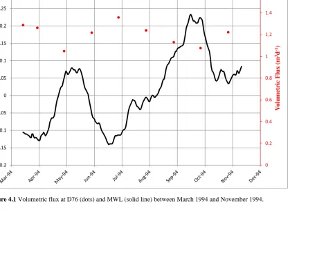
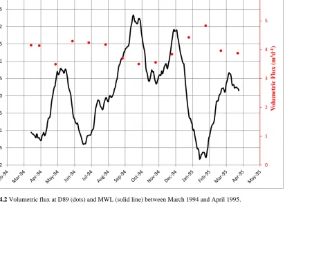
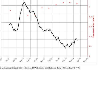
The calculated monthly average volumetric flux between Crabhaul Creek and

monitoring wells D76, D89, and D117 vary in magnitude but all display an inverse

relationship to the position of MWL (Figure 4.1, Figure 4.2, and Figure 4.3, respectively).

The volumetric flux values range from 0.83 to 4.83 m3d-1. The inverse relationship

between volumetric flux and MWL is evident in the period of record for each monitoring

well nest. Seasonal highs in the position of MWL lead to decreased volumetric flux

magnitudes while seasonal lows in the position of MWL lead to increased volumetric

flux magnitudes. As the position of MWL transitions from a trough to a peak (e.g. Figure

4.1 between mid-June and mid-September), the volumetric flux responds by decreasing

gradually from 1.36 to 1.08 m3d-1. Volumetric flux in these three locations is primarily

controlled by the position of MWL. Table 4-1 statistically summarizes the results of the

(28)

16

Table 4.1 Volumetric flux statistics for periods of record

Well ID

Average Flux

(m3d- 1)

Standard Deviation

( m3d-1)

Max Flux

(m3d- 1)

Min Flux

(m3d- 1)

Average Annual MWL

Period of Record

D76 1.22 0.1 1.36 1.05 0.0086 3/94-11/94

D89 4.01 0.38 4.83 3.50 0.0086 3/94-5/95

(29)

1

7

Figure 4.1 Volumetric flux at D76 (dots) and MWL (solid line) between March 1994 and November 1994.

(30)

1

8

Figure 4.2 Volumetric flux at D89 (dots) and MWL (solid line) between March 1994 and April 1995.

(31)

1

9

Figure 4.3 Volumetric flux at D117 (dots) and MWL (solid line) between June 1995 and April 1996.

(32)

20

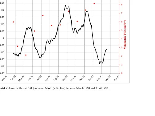
The calculated monthly average volumetric flux values in the high-marsh at D51

range from 2.16 to 8.28 m3d-1 and do not display the same inverse relationship to the

position of MWL that is seen in the mid and low-lying marsh wells (Figure 4.4). Here,

volumetric flux is controlled by precipitation, tidal amplitude, and MWL. This site is

closer than D76 to the terrestrial watershed that exists in the forested upland. The

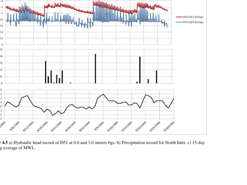
hydraulic head records from 0.6 meters bgs and 3.6 meters bgs exhibit two unique

hydraulic head signatures. The shallow well (0.6 meters bgs) generally has lower

hydraulic head values than the deeper well (3.6 meters bgs) in the same location. The

shallow well is also more responsive to the position of MWL and monthly tidal cycles.

This is particularly clear on August 6, 1994, when hydraulic head rises sharply during

inundating high tides. The deeper well is sensitive to precipitation events, and spikes in

the hydraulic head record correlate well with large precipitation events. Rainfall causes

rapid increases in the hydraulic head in the deeper part of the confined aquifer, followed

by a gradual decrease. The frequency of precipitation events determines the hydraulic

head in the deep well. The interaction of these factors control whether or not groundwater

(33)

2

1

Figure 4.4 Volumetric flux at D51 (dots) and MWL (solid line) between March 1994 and April 1995.

(34)

2

Figure 4.5 a) Hydraulic head record of D51 at 0.6 and 3.6 meters bgs. b) Precipitation record for North Inlet. c) 15-day running average of MWL

a)

b)

(35)

23

The difference between total discharge and net flux represents the total recharge

that occurs along the surface of the Crabhaul Creek bank and increases with increasing

tidal amplitude (Figure 4.6). During tidal cycles that had small amplitudes (0.44 m-0.56

m), very little recharge occurred. As tidal amplitude increased above 0.56 meters, total

recharge became greater. Total recharge continued to increase with each increase in tidal

amplitude from 0.56 meters to the maximum amplitude of 1.19 meters. The positive

correlation of total recharge and total discharge to tidal amplitude is evident for each

month in the D89 period of record.

A graph of total recharge plotted against the elevation of high tide (Figure 4.7)

shows a positive correlation between the two data sets. Increases in the elevation of high

tide drive increases in recharge magnitude. The plot also shows that a threshold exists, so

that certain high tide elevations must be met to produce certain recharge magnitudes. For

example, in order to achieve a total recharge of 0.5 meters per tidal cycle, the elevation of

(36)

2

4

Figure 4.6 Total discharge and total recharge response to tidal amplitude in D89 (January 1995).

-0.1 0.1 0.3 0.5 0.7 0.9 1.1 1.3 1.5 0 1 2 3 4 5 6 7 8 9 10

0.00 0.20 0.40 0.60 0.80 1.00 1.20 1.40

T ot al R ec h ar ge ( m /t id e) T ot al D is ch ar ge ( m /t id e)

(37)

2

5

Figure 4.7 Elevation of high tide versus total recharge in D89 (April 1994 to April 1995) 0

0.2 0.4 0.6 0.8 1 1.2 1.4

-0.5 0 0.5 1 1.5 2

H

igh

T

id

e E

le

vat

ion

(

m

)

(38)

26

4.2 Electrical Resistivity

All electrical resistivity surveys show two distinct zones (Figure 4.8). A zone of

low resistivity extends from 21 meters to 94 meters relative to the NW end of Transect D.

This zone extends from the surface to a maximum depth of 5 meters bgs. Resistivity

values in this zone ranged from 28.4 to 1.4 Ohm-m and were indicative of marsh mud

saturated by saline to brackish pore-water. A zone of higher resistivity originates in the

forested upland and extends into the subsurface marsh beneath the confining clay unit

and reaches a maximum depth of 20 meters bgs. The resistivity values in this zone range

from 6.4 to 40 Ohm-m, which we interpret to represent sand saturated with brackish to

fresh pore-water.

The plots of percent difference in resistivity show variability both zones

throughout the course of the year (Figure 4.9). Between June 30, 2012 and August 1,

2012, there is an increase in resistivity throughout the shallow zone with the exception of

an area between D45 and D50 that experienced a decrease in resistivity. The deeper zone

exhibited an increase in resistivity between D15 and D55 but a decrease in resistivity

from D55 to D89. Between August 1, 2012 and January 11, 2012, there was a general

increase in resistivity in the shallow and deep zones. There were decreases in resistivity

observed in the shallow zone between D85 and D105 and between D10 and D30 in the

deeper zone. The percent difference plot between January 11, 2013 and May 22, 2013

displayed a general increase in resistivity in the shallow subsurface except for a decrease

exhibited between D95 and D105. The deeper zone depicts an increase in resistivity

(39)

27

Each of the resistivity surveys was supplemented with in-situ salinity samples.

The salinity samples were collected from monitoring wells along Transect D that were

screened at a depth of approximately three meters bgs. The results were compared to the

corresponding electrical resistivity surveys (Figure 4.10). The standard deviation of the

resistivity and salinity data were calculated for each of the sampling dates (Table 4.2).

Data misfit cross-plots and data misfit pseudo-sections were generated and are included

as Appendix B. The resistivity results from each of the surveys show a steep decrease in

resistivity between the forested upland at D21 (average resistivity equals16.7 Ohm-m)

and the high marsh at D40 (average resistivity equals 3.5 Ohm-m). The resistivity values

then level out at values ranging from 1.4 to 4.2 Ohm-m between the high marsh at D40

and the low-lying marsh at D89. The salinity samples show more variability between

sampling events but generally salinity decreases from the upland at D21 to the high

marsh at D40, then increases between D40 and Crabhaul Creek at D89. The maximum

well depth along Transect D is 3.6 meters bgs, so it was not possible to obtain in-situ

samples from below the confining unit.

Table 4.2 Statistical analysis of resistivity and salinity results.

Sampling Date 6/30/2012 8/1/2012 1/11/2013 5/22/2013

Resistivity Mean (Ohm-m)

4.97 4.47 4.86 7.46

Resistivity Standard Deviation (Ohm-m)

4.42 4.16 2.98 9.35

Salinity Mean (ppt) 8.57 5.42 6.43 5.43

Salinity Standard Deviation (ppt)

(40)

Figure 4.8 Electrical resistivity inversions

January11, 2013, and d) May 22, represent mud layers.

a)

b)

c)

d)

28

Electrical resistivity inversions from a) June 30, 2012, b) August 1, 2012, 22, 2013. Dashed lines represent the clay unit. Solid lines

(41)

Figure 4.9 Percent difference plots (%) between a) June and August 2012 b) August

2012 and January 2013 and c) January and May 2013.

29

Percent difference plots (%) between a) June and August 2012 b) August 2012 and January 2013 and c) January and May 2013.

(42)

3

0

Figure 4.10 Salinity and resistivity plotted against distance along Transect D at a depth of 3 meters for a) June 30, 2012 b) August 1, 2012 c) January 11, 2013, and d) May 22, 2013

a) b)

(43)

31

CHAPTER 5

DISCUSSION

The results from this study show that groundwater discharge and recharge along

Transect D are controlled by a combination of MWL, tidal amplitude, and precipitation.

The factors that control advective groundwater flow transition from the forested upland to

Crabhaul Creek. In the low marsh adjacent to Crabhaul Creek and in the mid-marsh at

D76, the magnitude of tidally influenced groundwater discharge and recharge is

predominately controlled by the position of MWL. In the high-marsh at D51, vertical

groundwater flow is controlled by a complex interaction between MWL, tidal amplitude,

and precipitation.

The elevation of MWL can vary by as much as 0.5 meters over the course of a

year and strongly affects the magnitude of groundwater discharge in the mid- and low

marsh. Groundwater discharge displays an inverse relationship with the position of MWL

in the mid and low-lying marsh. This means that periods of low MWL produce higher

rates of groundwater discharge and higher MWL produces lower rates of groundwater

discharge. The range of tidal amplitude values is fairly constant throughout the year in

the North Inlet, but seasonal changes in MWL influence these tidal amplitudes by

increasing or decreasing their vertical reach across the marsh platform. This in turn

affects the area of the marsh platform that is inundated during high tides, the area of the

creek bank that is exposed during low tide, and the hydraulic gradient between the

(44)

32

marsh platform are inundated at high tide but a small area of the creek bank is exposed at

low tide. During periods of low MWL, smaller areas of the marsh platform are inundated

but more of the creek bank is exposed at low tide. More groundwater is discharged

through the creek bank at periods of low tide and low MWL because there is a larger

hydraulic gradient between the marsh groundwater and the surface water in Crabhaul

Creek. At periods of high MWL, there is a smaller hydraulic gradient and lower

groundwater discharge magnitudes. These results are consistent with the results of

Wilson and Morris (2012), who suggested an inverse relationship between MWL and

groundwater discharge. It appears that this relationship holds for forest-marsh boundaries

as well as for salt marsh islands.

Groundwater flow in the high marsh along Transect D is influenced by the

terrestrial watershed to the northwest, precipitation events, MWL position, and tidal

amplitude. The hydraulic head in the 3.6 meters bgs well at the D51 location is

influenced by precipitation and tidal cycles. The hydraulic head variations caused by the

precipitation events are much greater than the variations caused by tidal cycles. The

shallow well at D51, which is screened at 0.6 meters bgs, is much more responsive to

daily and monthly tidal cycles and is not influenced by precipitation. The ranges in

hydraulic head associated with the tidal cycles are much larger in the shallow well than in

the deep well. The increases and decreases in hydraulic head in this well correspond

nicely to the fluctuations in MWL due to spring and neap tidal cycles. The interaction

between these factors determines if discharge or recharge is occurring between the two

screened intervals. For example, consider a large precipitation even that occurs during a

(45)

33

the deep interval driven by the rain event and a low hydraulic head in the shallow well

due to the reduced amplitudes associated with the neap tidal cycles and the low position

MWL. This would create a discharge zone in the high marsh with a magnitude

proportional to the difference in hydraulic head between the deep and shallow wells.

Volumetric flux values calculated for the mid-marsh on the northwestern side of

the transect (D76) are 23 % larger than discharge calculated for the mid-marsh on the

southeastern side of the transect (D117). This was a surprising result, as we hypothesized

that groundwater discharge would be significantly greater on the northwestern side of the

transect due to the fact that a 75 square kilometerterrestrial watershed exists directly

up-gradient. Based on these results, the presence of a large freshwater lens in the upland

does not seem to significantly impact discharge. It appears that discharge from the large

upland bypasses the marsh, discharging at D51 or traveling through the fresher aquifer

below the confining unit.

Volumetric fluxes through the creek bank were converted to a flux per unit area of

the marsh via the creek density so that our fluxes could be compared to other estimates.

Creek density is the ratio of the length of creek bank to the area of marsh. The creek

density in the Crabhaul Creek Basin is 0.01 m-1, which is the same as the creek density

calculated for North Inlet by Novakowski et al (2004). We report volumetric flux and

flux per unit area to be consistent with both the groundwater and salt marsh literature.

The magnitude of groundwater discharge that we calculated based on data from D89 and

converted using the creek density term is slightly higher than previous values that have

been calculated for the North Inlet Basin (Table 5-2). The minimum value calculated in

(46)

34

Lm-2d-1. Based on previous studies, a maximum value of 40 Lm-2d-1 was calculated for

North Inlet by Krest et al. (2000) using radium isotope groundwater tracers. The larger

values can be attributed to the continuous nature of our monitoring and the seasonal

variations in groundwater discharge that emerged. The former studies from North Inlet

only achieved temporal “snap shots” of groundwater discharge which cannot be

considered representative of the system due to the variable tendencies that we observed.

Krest et al. (2000) also noted that significant groundwater discharged through the creek

bottom, which raised the question of whether the discharging groundwater originated in

the marsh or in a deeper aquifer. Our results suggest that tidal fluctuations in the marsh

are adequate to explain the fluxes observed by Krest et al (2000).

Table 5.1 Results of current and former groundwater studies in North Inlet

Study Author(s) Location Method Discharge

(Lm-2d-1)

Whiting and Childers (1989)

North Inlet, SC Seepage meter 7.8-28

Morris (1995) North Inlet, SC Salt and water balance 9.4-16.6

Krest et al (2000) North Inlet, SC Radium tracers 20-40

Wilson and Gardner (2006)

North Inlet, SC Numerical simulations 10-14

This study North Inlet, SC Darcy flux

calculations

36.01-49.77

Groundwater recharge also occurs at the creek bank along Transect D and

displays a positive correlation with high tide elevation. At lower high tide elevations, the

total recharge that occurs is non-existent or minimal. This is due to the fact that the height

of the surface water in the creek is not large enough to reverse the hydraulic gradient.

(47)

35

higher MWL. As the elevation of high tide gradually increases from 0.3 meters to 1.2

meters, more and more seawater begins to infiltrate at the creek bank. Higher MWL

combined with larger tidal amplitudes create surface water heights in the creek capable of

reversing the component of flow during the peaks of each tidal cycle. This leads to

substantial groundwater exchange along the creek bank.

We hypothesized that salinity in the shallow subsurface (up to four meters bgs)

would display seasonal variations that were related to seasonal variations in discharge,

but the electrical resistivity surveys and in-situ salinity sampling data contradict this

hypothesis. Tobias et al. (2001) suggested that “groundwater mediated” flushing

associated with seasonal variations in groundwater discharge flushed the subsurface

marsh of salts and nutrients. Carter et al. (2007) also showed that a freshwater/saltwater

interface existed along Transect C in North Inlet and that the lateral extent of this

interface migrated on a monthly timescale. Our results suggest that the saline to brackish

zone that exists in the shallow subsurface experiences temporal and spatial variability that

is not easily correlated to precipitation or the position of MWL (Figure 5.1).

Variation in electrical resistivity was much more apparent in the deeper zone

between the clay confining unit and approximately 20 meters bgs. The percent difference

plot presented in Figure 4.9 shows two areas in the deep subsurface that alternate

between increasing and decreasing resistivity over the course of a year. The first area is

located at a depth of five to 15 meters bgs and laterally between 10 and 30 meters from

the NW end of Transect D. The second area is located between five and 15 meters bgs

and laterally between 65 and 100 meters from the NW end of Transect D. These

(48)

36

MWL. It is clear that lithologic changes do not occur on this time scale, so the resistivity

variations must be due to groundwater processes. We believe that the deeper, higher

resistivity zone (freshwater zone) is hydraulically disconnected from the upper saline to

brackish zone and could be part of a larger flow path that connects the forested upland to

some discharge point to the southeast of Transect D. The relationship between rainfall

and changes in resistivity in the deeper zone needs further investigation.

(49)

Figure 5.1 Electrical resistivity surveys

c) January11, 2013, and d) May 22, 2013 MWL position.

a)

b)

c)

d)

e)

37

Electrical resistivity surveys a) June 30, 2012, b) August 1, 2012, c) January11, 2013, and d) May 22, 2013 and e) 29-day running average of

(50)

3

8

Figure 5.2 Daily precipitation totals for d) April 23 to May 7, 2013.

a)

c)

Daily precipitation totals for a) June 1 to 30, 2012 b) July 2 to August 1, 2012 c) December 12 to 27, 2012 b)

d)

(51)

39

CHAPTER 6

CONCLUSION

This study quantitatively shows that discharge from a fringing marsh is variable

on a seasonal basis and the factors that control the flow of groundwater through the

marsh are determined by the location within the system. Groundwater discharge at the

low-lying and mid-marsh locations is predominantly controlled by the elevation of MWL.

There is an inverse relationship that exists at these locations between the position of

MWL and the magnitude of groundwater discharge. In the high-marsh, groundwater

discharge is influenced by MWL, tidal amplitude, and precipitation. The interactions of

these factors determine whether groundwater discharges or recharges and the magnitude

of this flow.

There are two primary zones that occur in the subsurface along Transect D which

are separated by a confining clay unit. The top zone has a pore-water salinity that is

saline to brackish. In this zone, freshwater that makes it past the high-marsh location is

mixed with seawater that infiltrates through the creek bank and the marsh mud. The

brackish and saline water is transported slowly through the subsurface and eventually

discharges at the creek bank of Crabhaul Creek. The deeper zone displays resistivity

signatures indicative of freshwater. There are two flow paths that the freshwater in the

upland can take. First, it can be transported above the confining clay unit, where it is

(52)

40

flow under the confining clay unit where it is isolated from the saline water above and

discharged further to the east.

The variable magnitude of groundwater discharge along the transect and the

mixing that occurs in the upper zone are important when considering nutrient export.

Groundwater must have a salinity concentration of greater than ten ppt to transport

nutrients. This implies that along Transect D all of the nutrients are being exported from

the shallow, saline to brackish zone. Nutrient export is proportional to groundwater

discharge. The seasonal variation that we see in discharge can potentially introduce

pulses of nutrient enriched groundwater into the adjacent coastal water. Also, long term

sea level rise that occurs at a rate that is faster than sediment accretion would decrease

(53)

41

R

EFERENCES

Carr, P.A. and V.D. Kamp, Determining aquifer characteristics by the tidal method, Water Resources Research, 5(5), 1023-1031, 1969

Carter, E.S., S.M. White, and A.M. Wilson, Variation in groundwater salinity in a tidal salt marsh basin, North Inlet Estuary, South Carolina, Estuarine, Coastal and Shelf Science, 76, 543-552, 2008.

Dame, R.F., and L.R. Gardner, Nutrient processing and the development of tidal creek ecosystems, Marine Chemistry, 43, 175-183, 1993.

De Meneses, J.G.A., Modeling the fresh water inflow to the Pettaquamscutt River. Ph.D. thesis, University of Rhode Island.

Gardner, L.R., and D.E. Porter, Stratigraphy and geologic history of a southeastern salt marsh basin, North Inlet, South Carolina, USA, Wetlands Ecology and

Management, 9, 371-385, 2001.

Harvey, J.W. and W.K. Nuttle, Fluxes of water and solute in a coastal wetland sediment. Journal of Hydrology, 164, 109-125, 1995.

Kelly, R.P., and S.B. Moran, Seasonal changes in groundwater input to a well-mixed estuary estimated using radium isotopes and implications for coastal nutrient budgets, Limnology and Oceanography, 47(6), 1796-1807, 2002.

Keenan, R.S., An investigation of the dynamics of groundwater flow and salinity distribution along a forest-marsh transect. Ph.D. thesis, Columbia: University of South Carolina

Krest, J.M., W.S. Moore, L.R. Gardner, and J.T. Morris, Marsh nutrient export supplied by groundwater discharge, Global Biogeochemical Cycles, 14(1), 167-176, 2000.

Morris, J.T., The mass balance of salt and water in intertidal sediments: results from North Inlet, South Carolina, Estuaries, 18(4), 556-567, 1995.

(54)

42

Novakowski, K.I., R. Torres, L.R. Gardner, and G. Voulgaris, Geomorphic analysis of tidal creek networks, Water Resources Res., 40, W05401,

doi:10.1029/2003WR002722, 2004.

Reilly, T.E., and A.S. Goodman, Quantitative analysis of saltwater-freshwater relationships in groundwater systems-a historical perspective, Journal of Hydrology, 80, 125-160, 1985.

Thibodeau, P.M., Groundwater flow dynamics across the forest-salt marsh interface: North Inlet, SC. Ph.D. thesis, Columbia: University of South Carolina

Tobias, C.R., J.W. Harvey, and I.C. Anderson, Quantifying groundwater discharge through fringing wetlands to estuaries: seasonal variability, methods comparison, and implications for wetland-estuary exchange, Limnology and Oceanography, 46(3), 604-615, 2001.

U.S. Geological Survey, Water resources data reports for South Carolina, Columbia, SC, 1983-1993.

Whiting, G.J., and D.L. Childers, Subtidal advective water flux as a potentially important nutrient input to southeastern U.S.A. saltmarsh estuaries, Estuarine Coastal Shelf Science, 28(4), 417-431, 1989.

Wilson, A.M., and J.T. Morris, The influence of tidal forcing on groundwater flow and nutrient exchange in a salt marsh-dominated estuary, Biogeochemistry, 108, 27-38, 2012.

Wilson, A.M., and L.R. Gardner, Tidally driven groundwater flow and solute exchange in a marsh: numerical simulations, Water Resources Research, 42, W01405,

(55)

43

APPENDIX A

ELECTRICAL RESISTIVITY PARAMETERS

June 30, 2012 Survey Parameters

Advanced Geosciences Inc. (AGI) Sting/SuperSting measured data (*.stg) Type: XYZ A trimmed data set by AGI EarthImager 2D. Version: 2.4.0 (Build 617). Records: 279 Raw data file: C:\Documents and Settings\jpeurifoy\Desktop\Thesis

Information\Research

Data\Resistivity\6.30.12\TRAND1_Reversed\trial3\TRAND1_Reversed_trial3.stg Terrain file: C:\Documents and Settings\jpeurifoy\Desktop\Thesis Information\Research Data\Resistivity\6.30.12\TRAND1\TranD12.trn

Number of Data = 279 Number of Electrodes = 28

Number of Surface Electrodes = 28 Number of IP Data = 0

Processing starts at 2012-09-13 12:30:13

;--- SETTINGS ---

Minimum Voltage (mv) = -1 Minimum V/I (ohm) = 0.0002

Minimum apparent resistivity (ohm-m) = 0.1 Maximum apparent resistivity (ohm-m) = 10000 Maximum repeat error (%) = 7

Maximum reciprocal error (%) = 10

Remove negative apparent resistivity in ERT data: Yes Keep All Data (no data removal): No

Inversion Method: Smooth model inversion Vertical axis: Positive Upward

Y Coordinate = Depth

Min electrode spacing X (m) = 0.003 Min electrode spacing Z (m) = 0.003

Forward Modeling Method: Finite element method Forward system solver: Cholesky decomposition method Boundary condition type: Dirichlet

(56)

44 Max number of iteration of nonlinear inversion = 10 Stop RMS error = 3%

Mininum error reduction between two iterations = 5% Stop at Max number of iterations: Yes

Stop when RMS is small enough: No Stop when RMS can not be reduced: No Res Data reweighting: No

Use Reciprocal Error: No

Stop when L2 norm is small enough: No Initial smoothness factor = 1000.0 Roughness conditioner = 0.2 Starting model: Avg AppRes.

Start halfspace resistivity = 7.08 ohm-m Minimum resistivity = 1.0 ohm-m Maximum resistivity = 100000.0 ohm-m Number of elements combined horizontally = 1 Number of elements combined verically = 1 Vertical / Horizontal roughness ratio = 0.2 Estimated noise of resistivity data = 3% Initial damping factor of resistivity = 1000.0 Starting iteration of quasi Newton method = 20 IP inversion method: No IP Inversion

Terrain mesh transform method: Damped transform.

;--- ELECTRODE LOCATIONS ---

(57)

45

19, 76.000, 0.000, 76.000, -1.367 20, 80.000, 0.000, 80.000, -1.413 21, 84.000, 0.000, 84.000, -1.457 22, 88.000, 0.000, 88.000, -1.502 23, 92.000, 0.000, 92.000, -1.454 24, 96.000, 0.000, 96.000, -1.393 25, 100.000, 0.000, 100.000, -1.347 26, 104.000, 0.000, 104.000, -1.394 27, 108.000, 0.000, 108.000, -1.440

August 1, 2012 Survey Parameters

Information\Research Data\Resistivity\8.1.12\4m MRT Poster 8.1.12\11TRAND_Reversed\trial3\11TRAND_Reversed_trial3.stg

Terrain file: C:\Documents and Settings\jpeurifoy\Desktop\Thesis Information\Research Data\Resistivity\8.1.12\4m MRT Poster 8.1.12\TranD12.trn

;--- SETTINGS ---

Minimum Voltage (mv) = 1 Minimum V/I (ohm) = 0.0005

(58)

46

Lower-layer-thickness / Upper-layer-thickness = 1.1 Depth of Inverted Model / Depth of Pseudosection = 1.1 Max number of iteration of nonlinear inversion = 15 Stop RMS error = 5%

Mininum error reduction between two iterations = 3% Stop at Max number of iterations: No

Stop when RMS is small enough: No Stop when RMS can not be reduced: No Res Data reweighting: Yes

Stop when L2 norm is small enough: Yes Initial smoothness factor = 100

Roughness conditioner = 0.1 Starting model: Avg AppRes.

Start halfspace resistivity = 7.01 ohm-m Minimum resistivity = 1.0 ohm-m Maximum resistivity = 100000.0 ohm-m Number of elements combined horizontally = 1 Number of elements combined verically = 1 Vertical / Horizontal roughness ratio = 0.2 Estimated noise of resistivity data = 5% Initial damping factor of resistivity = 100 Starting iteration of quasi Newton method = 20 IP inversion method: No IP Inversion

(59)

47

17, 68.000, 0.000, 68.000, -1.262 18, 72.000, 0.000, 72.000, -1.315 19, 76.000, 0.000, 76.000, -1.367 20, 80.000, 0.000, 80.000, -1.413 21, 84.000, 0.000, 84.000, -1.457 22, 88.000, 0.000, 88.000, -1.502 23, 92.000, 0.000, 92.000, -1.454 24, 96.000, 0.000, 96.000, -1.393 25, 100.000, 0.000, 100.000, -1.347 26, 104.000, 0.000, 104.000, -1.394 27, 108.000, 0.000, 108.000, -1.440

January 11, 2013 Survey Parameters

Information\Research Data\Resistivity\1.11.13\4m MRT 1.11.13\110133_Reversed\trial1\110133_Reversed_trial1.stg

Terrain file: C:\Documents and Settings\jpeurifoy\Desktop\Thesis Information\Research Data\Resistivity\1.11.13\4m MRT 1.11.13\TRAND4m.trn

;--- SETTINGS ---

Minimum apparent resistivity (ohm-m) = 1 Maximum apparent resistivity (ohm-m) = 100000 Maximum repeat error (%) = 7

(60)

48 Boundary condition type: Dirichlet

Number cells or elements betwenn two electrodes = 2 Lower-layer-thickness / Upper-layer-thickness = 1.1 Depth of Inverted Model / Depth of Pseudosection = 1.1 Max number of iteration of nonlinear inversion = 15 Stop RMS error = 5%

Stop when RMS is small enough: No Stop when RMS can not be reduced: Yes Res Data reweighting: No

Stop when L2 norm is small enough: No Initial smoothness factor = 100

(61)

49

15, 60.000, 0.000, 60.000, -1.157 16, 64.000, 0.000, 64.000, -1.210 17, 68.000, 0.000, 68.000, -1.262 18, 72.000, 0.000, 72.000, -1.315 19, 76.000, 0.000, 76.000, -1.367 20, 80.000, 0.000, 80.000, -1.413 21, 84.000, 0.000, 84.000, -1.457 22, 88.000, 0.000, 88.000, -1.502 23, 92.000, 0.000, 92.000, -1.454 24, 96.000, 0.000, 96.000, -1.393 25, 100.000, 0.000, 100.000, -1.347 26, 104.000, 0.000, 104.000, -1.394 27, 108.000, 0.000, 108.000, -1.440

May 22, 2013 Survey Parameters

Information\Research Data\Resistivity\5.22.13\4m MRT

5.22.13\BRAD4M_Reversed_Scaled\trial6\BRAD4M_Reversed_Scaled_trial6.st g

Terrain file: C:\Documents and Settings\jpeurifoy\Desktop\Thesis Information\Research Data\Resistivity\5.22.13\4m MRT 5.22.13\TranD12.trn

;--- SETTINGS ---

(62)

50 Min electrode spacing Z (m) = 0.003

Number cells or elements betwenn two electrodes = 2 Lower-layer-thickness / Upper-layer-thickness = 1.1 Depth of Inverted Model / Depth of Pseudosection = 1.1 Max number of iteration of nonlinear inversion = 15 Stop RMS error = 5%

Stop when RMS is small enough: No Stop when RMS can not be reduced: No Res Data reweighting: Yes

Stop when L2 norm is small enough: Yes Initial smoothness factor = 100

(63)

51

(64)

52