Article
1
Moving Source Depth Estimation Using a Horizontal Line
2
Array in Shallow Water Waveguides
3
Guolong Liang
1,2,3, Yifeng Zhang 1,2,3 , Nan Zou1,2,3,* and Jinjin Wang 1,2,34
1 Acoustic Science and Technology Laboratory, Harbin Engineering University, Harbin, China;
5
2 Key Laboratory of Marine Information Acquisition and Security (Harbin Engineering University), Ministry
6
of Industry and Information Technology; Harbin 150001, China
7
3 College of Underwater Acoustic Engineering, Harbin Engineering University, Harbin, China;
8
[email protected]; [email protected]
9
* Correspondence: [email protected]; Tel.: +86-151-2450-3518
10
Abstract: In this study, a matched-mode autoregressive source depth estimation method (MMAR)
11
based on autoregressive (AR) wavenumber estimation is proposed for a moving source in shallow
12
water waveguides. The signal original frequency and the environmental parameters, namely, the
13
sound speed profile and bottom properties are known as a prior knowledge. The mode
14
wavenumbers are estimated by the AR modal wavenumber spectrum. On the basis of the mode
15
wavenumber estimation, the mode amplitudes can be estimated by the wavenumber spectrum
16
that is obtained by generalized Hankel transform. The source depth estimation is determined by
17
the peak of source depth function wherein the data mode best matches the replica mode that is
18
calculated using a propagation model. Compared with other methods of moving source depth
19
estimation, the proposed method exhibits a better performance in source depth estimation under
20
low signal-to-noise ratio or the small range span. The selection of horizontal line array depth is
21
illustrated by simulation and normal mode theory in details.
22
Keywords: modal wavenumber spectrum; match mode; horizontal line array; moving source
23
24
1. Introduction
25
Matched field processing (MFP) [1-2] or the equivalent matched mode processing (MMP) [3] is
26
a popular method for localizing the source in complex propagation environments. Conventional
27
MFP obtains the range depth function, that is, the correlation between the replica and the measured
28
fields. The source location is determined by the peak of the range depth function. MFP can localize
29
the source accurately in a range-independent or slowly varying environment without considering
30
any environmental mismatches. When the sound propagation is not exactly modeled, the range and
31
depth estimated by MFP generally present an error, which is referred to as the environmental
32
mismatch problem [4]. The need for depth estimation is more pressing than range estimation for
33
some applications. The source range and depth are estimated simultaneously by MFP, which
34
indicates that depth estimation depends on range estimation. The robustness of depth estimation
35
decreases because of the sensitivity of range estimation to sound speed profile (SSP). MFP always
36
requires a vertical line array (VLA) or a horizontal line array (HLA) with large aperture. However,
37
real application of large aperture array is difficult because of the installation platform. The
38
application of MFP is restricted by the aperture problem and the environmental mismatch problem.
39
Consequently, an active area of research in recent years has been devoted to estimate source depth
40
robustly by a single hydrophone or a short line array [5-7].
41
A class of methods that has shown some promise in passive location exploits the properties of
42
the reliable acoustic path (RAP) [8]. Such methods reduce the requirement of array aperture. The
43
difficulty associated with the propagation of RAP limits the application of the method in shallow
44
water. Depth estimation for shallow water waveguides is generally performed in two steps: mode
45
filtering first and then MMP [3]. The modal amplitudes are determined by mode filters, and then the
46
MMP is used to estimate the source location on basis of the modal amplitudes. However, the mode
47
filters always require well-sampling of the water column by the VLA; otherwise, the mode filtering
48
will become an ill-posed problem. The difficulty in source depth estimation using a short line array
49
is the lack of spatial information. Thus, some previous studies have relied on the multi-frequency
50
characteristics of wideband signals in estimating source depth [9-10]. Considering the dispersion
51
phenomenon of signals in shallow water, some scholars have estimated source depth on the basis of
52
the related information of marine environment contained in dispersion [11]. However, the above
53
mentioned studies have restricted the signal form to be broadband and few works on source depth
54
estimation for signal with low-frequency line spectrum are available. Recently, data-based
55
MFP/MMP is being proposed for a moving source by using a full-spanning VLA, which is free of the
56
environmental mismatch problem in theory [12-13]. Yang [7] proposed a method based on the idea
57
of data-based MFP/MMP to estimate moving source depth, and this method requires only a single
58
hydrophone. It is more robust than MFP for depth estimation because of not requiring source range
59
estimation. However, the method presents some inherent drawbacks. (1) The method requires
60
source travelling a sufficient range in radial direction owing to that the mode wavenumbers are
61
estimated by synthetic aperture modal beamforming (SAB). Some of the horizontal wavenumbers
62
cannot be estimated, when the moving range does not meet the requirement. Source depth
63
estimation based on synthetic aperture beaming may be incorrect. (2) The model assumes that the
64
signal possesses high signal-to-noise (SNR). Such requirement of SNR is difficult to meet in passive
65
positioning. (3) The algorithm is difficult to apply when the source is not moving in the radial
66
direction.
67
In this study, we propose a source depth estimation approach with an HLA for a moving source
68
in a range-independent environment, without knowing source absolute range information. When
69
beam steers to the source direction, the signal is enhanced after beamforming. We apply the
70
autoregressive (AR) model to the signal enhanced by array gain to estimate the wavenumbers. The
71
AR wavenumber spectrum is unsuitable to estimate mode amplitudes. Thus, the
72
generalized/modified Hankel transform is applied to the data. The source depth is estimated by the
73
peak of the depth ambiguity function wherein the mode depth functions best match the mode
74
amplitudes. Compared with SAB, the proposed method effectively improves the depth estimation
75
performance for the data with short range span or low SNR, and exhibits better adaptability to the
76
notion of the observation platform. In addition, the proposed method can be applied to underwater
77
unmanned vehicles or the autonomous underwater vehicles because it identifies the peaks of
78
wavenumber spectrum automatically.
79
The remainder of the paper is organized as follows. The wavenumber estimation for the
80
beamforming output is developed in Section 2. In Section 2.1, the generalized Hankel transform is
81
extended to beamforming output in a range independent environment [7]. A method for
82
wavenumber estimation based on an AR model without knowing the source range is proposed in
83
Section 2.2. Source depth estimation based on wavenumber spectrum is introduced in Sec 3. The
84
factors that influence the performance of the algorithm are explored in Section 4. The performance of
85
the algorithm on the data with different SNRs and different range spans is analyzed in Section 4.1.
86
Given that the HLA depth also affects the performance of the algorithm, the effect of the laying
87
depth of HLA on the algorithm and its selection method are examined in details in Section 4.2. A
88
summary and discussion is provided in Section 5.
89
2. Mode Wavenumber Estimation
90
We assume that source travels at a fixed depth during observation in a range-independent
91
environment. The considered HLA possesses
N
receivers that are uniformly spaced withd
. The92
first element of HLA is the reference. The far-field source radiates the continuous wave signal, with a
93
look direction
i.
i is the true value of the look direction at thei
th moment. The range between94
source and reference array element is
r
i at thei
th moment. In shallow water waveguides, we95
suppress a time dependence of the form
e
j t with
positive, thus, the pressure field of then
th96
element at the
i
th moment can be represented using normal mode theory as4 1
exp{
(
)[
(
1) sin
]}
( ,
)
2
( )
( )
[
(
1) sin
]
M j
m m i i
n i r m s m r
m m i i
j k
j
r
n
d
p r z
e
z
z
k r
n
d
, (1)where
k
m,
m, and
m are the wavenumber, the attenuation coefficient, and the mode depth98
function, respectively, which all belong to the
m
th mode;z
s andz
r are the source and HLA99
depths, respectively; and
M
is the number of modes considered in the propagation model.100
The source is at the far field, such that
r
i
n
1
d
sin
r
i. Equation. (1) is simplified as101
4 1
1
exp{
(
)[
(
1) sin
]}
( ,
)
2
( )
( )
exp{
(
)[
(
1) sin
]}
M j
m m i i
n i r m s m r
m m i
M
m m m i i
m
j k
j
r
n
d
p r z
e
z
z
k r
A
j k
j
r
n
d
, (2)
where
2
j4 m( )
s m( )
r m m iz
z
A
e
k r
. To improve the SNR, beamforming is performed on the102
signal received on the HLA at the
i
th moment.103
11
ˆ
ˆ
( )
( )(
( ,
)
( ,
))
Ni n i n i r n i r n
B
w
p r z
n r z
N
, (3)( ,
)
n i r
n r z
is modeled as the Gaussian white noise. For conventional beamforming, the output of104
beamforming is written as
105
ˆ ( 1) sin
1
1
ˆ
( )
i(
( ,
)
( ,
))
N
jk n d
i n i r n i r
n
B
e
p r z
n r z
N
, (4)After substituting Equation. (2) into Equation. (4),while ignoring noise, we obtain
106
1
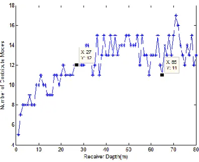
1
ˆ
( )
m i m isinb(
)
M
jk r r
i m m
m
B
A e
X
N
, (5)where
X
m
(
k
mj
m) sin
i
k
sin
ˆ
i ,sinb(
)
sin(
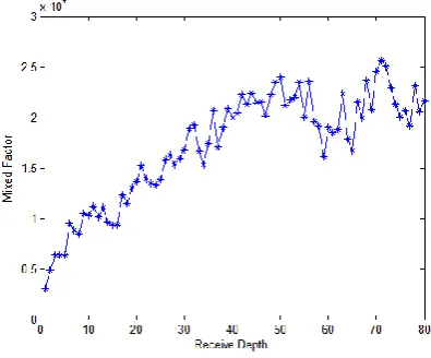
) sin(
)
2
2
m m m
Nd
d
X
X
X
.
ˆ
i is the107
estimation of the look direction, which can be obtained by many methods [14]. In order to explain
108
the algorithm conveniently, we discuss the method of estimating the sound source depth when
109
source moves away from the HLA under the assumption that
ˆ
i
i .110
2.1. Wavenumber estimation using generalized Hankel transform
111
In range-independent shallow water waveguides, a Hankel transform pair presents the
112
relationship between the complex pressure field
p r z
( ;
s,
z
r)
and the Green’s function113
( ; ,
r s r)
g k z z
[15]114
0 0 0 0( ;
,
)
( ;
,
) (
)
( ;
,
)
( ;
,
) (
)
s r r s r r r r
r s r s r r
p r z z
g k z z J k r k dk
g k z z
p r z z J k r rdr
, (6)where
J
0 is the zeroth-order Bessel function.115
Considering the computation of Hankel transform, the Green’s function is often approximated
116
by an inverse Fourier transform (FT) as [15]
4
( ;
,
)
( ;
,
)
,
1
2
r
i
ik r
r s r s r r
r
e
g k z z
p r z z e
rdr
k r
k
, (7)We consider the source motion model, source range
r
r
ir
0iv t
, where
t
is the118
sampling interval, and
r
0 is the unknown initial source range att
0
. We assume that the source119
radiates a tone signal. Thus, the source speed
v
can be estimated by Doppler shift with knowing120
original signal frequency. According to Equation. (7), the Hankel transform, which is used
121
previously to estimate the wavenumber, requires knowledge of the source range. The source range
122
is difficult to be measured correctly for passive position system. We apply the generalized Hankel
123
transform proposed in [7] to the beamforming output. The generalized Hankel transform for the
124
beamforming output is described as
125
0
0
4
0
( ,
)
( )
( )
,
1
2
r
i
r R
ik r
r r r r
r
e
g k z
B r e
S r dr
k r
k
, (8)where
R
is the range span wherein source moves during the observation time.S r
is intended126
to compensate for the cylindrical spreading loss and will be obtained directly from the data.
127
1 2
2
( )
( )
S r
B r
, (9)where is the range averaging or smoothing operation. Equation. (8) reduces to the original
128
Hankel transform by setting
S r
( )
r
. In the present discussion,S r
( )
is approximately129
proportional to
r
using range averaging. After substituting Equation. (5) into Equation. (8),130
while assuming
S r
( )
r
, we obtain131
0 0 ( ) 1 1( )
( )
( ,
)
sinb(
)
( )
( )
r m m
M r R
j k k r r m s m r
r r m r
m r m M
m s m r m
m r m m
z
z
g k z
X
e
dr
k k
z
z
a
k
k
j
, (10)where
132
( ) 0 ( ) 0
sin (
)
r m m r m m
j k k r R j k k r
m m
r m
e
e
a
b X
j k k
, (11)When
k
r
k
m, the value of them
th item is much larger than the others in Equation. (10).Thus,133
the wavenumber spectral peak at
k
r
k
m is given by134
135
(
m, )
r m m( )
rg k z
b
z
, (12)0 '
2
sinh(
)
( ) sin (
)
2
r
m
m m s m
m m
R
e
b
z
b X
k
, (13)where
'
02
R
r
r
. This expression can be described by the matrix form.
g
Φ b
, (14) where137
( ,
1), ( ,
2),
, (
,
)
Tr r M r
g k z
g k z
g k
z
g
, (15)
1( ),
r 2( ),
r,
M( )
r
diag
z
z
z
Φ
, (16)
1,
2,
,
T Mb b
b
b
. (17)The aforementioned wavenumber estimation method is based on the FT, and is convenient to
138
be calculated by FFT. However, the FT-based approach presets some inherent disadvantages: (1) The
139
spectral resolution of FT is limited by the range span. To resolve the modal wavenumbers between
140
the
i
th andj
th modes, the range needs to be larger than the interference distance 2i j
ij k k
d
. If141
all the wavenumbers are estimated, then the range must be larger than all interference distances. (2)
142
The spectrum leakage occurs seriously when the method is applied to the data with a short range
143
span. The sidelobes of strong spectral components can contaminate the weak spectral components or
144
generate a false spectral peak. With the increase in source frequency or waveguide depth, the lower
145
mode wavenumbers will closely group together. As a result, the wavenumbers are difficult to be
146
estimated in this environment. Considering the drawbacks of FT, the modern spectral estimation
147
methods can be applied to wavenumber estimation.
148
2.2. Wavenumber estimation using AR model
149
Several methods have been developed to extract the mode wavenumbers, such as Prony’s
150
method, the signal subspace algorithms and matrix-pencil [16,17]. However, these methods regard
151
the number of wavenumbers as a priori. The number of wavenumbers cannot be known correctly in
152
practice. The AR spectral estimators based on an all-pole model are often used to extract the spectral
153
peaks in frequency estimation [17]. The AR estimator does not need to know the number of
154
wavenumbers, and is thus attractive to estimate wavenumbers. However, the source range must be
155
known for the AR estimator. Consequently, improved AR estimator should be used to extract the
156
mode wavenumbers.
157
The method can be divided into three steps. First, data are preprocessed by
158
y i
[ ]
B r S r
( ) ( )
i ii
1, 2
L
, (18) Second, considering thaty i
[ ]
can be described as the output of a linear system, we construct the159
AR model as
160
1
[ ]
[ ] [
]
[ ]
p
k
y i
a k y i
k
u i
, (19)where
p
is the order of the AR model to represent the data, and is often set to2
3
N
[17]. Finally,
161
we assume that
u i
[ ]
is a zero mean white noise sequence with
2. Thus, the wavenumber spectral162
density
P
AR is expressed as:163
2
1
( )
1
[ ]exp[
]
AR p
k
P
l
a k
ilk
,
AR
P
is obtained by estimating the coefficientsa
[1]
,a
[2]
, ,a p
[ ]
and
2 . The164
above-mentioned coefficients can be estimated in different ways. We select the modified covariance
165
approach because it avoids the spectral line splitting effectively [18]. The locations of peaks in
P
AR166
yield the wavenumbers estimated by AR model. The peak levels estimated by AR estimator possess
167
large variances [18]. Thus, AR estimator is unsuitable to estimate the modal amplitudes.
168
3. Matched-Mode Source Depth Estimation
169
As discussed above, the wavenumbers can be estimated by AR spectrum. However, AR
170
spectrum is unsuitable to estimate the modal amplitudes. The performance of estimating
171
wavenumbers degrades by using the generalized Hankel transform. The performance is effected by
172
false spectral peaks and spectral resolution. To combine the advantages of two methods, the modal
173
amplitudes are estimated by generalized Hankel transform with a prior knowledge of wavenumbers
174
that are estimated by AR model. Thus, we estimate the wavenumber
k
m by AR model, and then175
obtain
g k
(
m,
z
r)
in the wavenumber spectrum on basis of the generalized Hankel transform.176
According Equation. (14), we use a source depth ambiguity function to estimate source depth,
177
and this function is expressed as
178
D z
( )
φ
( )
z
bbφ
H( )
z
, (21) where179
1 2
( )
z
( ),
z
( ),
z
,
M( )
z
. (22)b
can be solved by180
b
(
Φ U
)
1g
, (23)
/
1( ),
r/
2( ),
r,
/
M( )
r
diag
z
z
z
U
, (24)where
is a small amount (on the order of one half of the maximum value of the mode function)181
for preventing the singularity of
Φ
. Wavenumbersk
m' and
m( )
z
are calculated by KRAKEN on182
the basis of a given frequency and environmental information (SSP and bottom properties). Some
183
modes cannot be resolved even if we use the AR spectrum, such that the number of
g k
(
m,
z
r)
is184
less than
M
. We assume that onlyM
0 order is estimated.
m( )
z
with the same order of185
(
m,
r)
g k
z
can be determined by solving the problem as follows186
0 0
0 0 0 0
min(
) (
)
. .
(1)
(2)
(
)
s t
M
H
k - k
k - k
k
k
k
, (25)where
187
0
1
,
2,
,
T M
k k
k
k
, (26)' ' '
1
,
2,
T M
k k
k
'
k
, (27)0
'
k
k
. (28)k
is anM
0
1
vector,k
' is anM
1
vector,andk
0 is anM
0
1
vector.188
This section presents comparisons of the source depth estimation results of the SAB and the
190
proposed matched-mode autoregressive source depth estimation method (MMAR). Different range
191
span and SNR should be considered in evaluating the performance of SAB and MMAR in estimating
192
source depth. For SAB, source depth can be estimated using only a single hydrophone under the
193
assumption that source moves away from receiver at a constant speed during the observation time.
194
For convenient comparison, we assume the source of SAB moves along the beam direction of HLA.
195
Apart from the influence of SNR and range span on the performance of the algorithms, the influence
196
of the HLA depth on MMAR is also considered. We study this effect from theory and simulation.
197
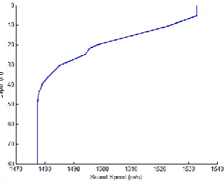
The pressure field is generated using the KRAKEN program. The SSP for simulation is shown
198
in Figure 1, and the bottom properties are referred to Reference 7. The consider a HLA possesses
N
199
receivers that are uniformly spaced with
d
, where2
d
. In studying the difference in depth200
estimation performance, we consider two sources depths of 4 and 50 m, which correspond to
201
shallow and deep sources, respectively. The initial source range is 5010 m, but this information is
202
assumed to be unknown. The performance influenced by the unknown initial source range has been
203
discussed in Ref. 7. We assume that each source moves away from the HLA with a speed of 2.5 m/s,
204
and radiates the narrowband signal with 350 Hz. The SNR in this simulation is defined as:
205
0
10 lg
s r r nP
SNR
P
. (29)According to Equation. (29), when source range is 5010 m, the SNR is described by the ratio of signal
206
power and noise power at receiver. The array gain is already considered in SNR.
207
208
Figure 1. Sound speed profile used in this experiment, which is typical in shallow waveguides.
209
4.1. Comparison of SAB and MMAR applied to simulation data
210
The HLA depth is 70 m without special instructions. The effectiveness of our algorithm is
211
analyzed in the following three cases and compared with that of SAB. A unified description is given
212
to avoid duplication, that is, the deep source is expressed by the blue line and the shallow source is
213
expressed by the red line. In Figure 2-4, subplot (a) shows the wavenumber spectrum obtained by
214
the generalized Hankel transform; subplot (b) shows the AR wavenumber spectrum obtained by AR
215
model, which is used to estimate the mode wavenumbers in MMAR; the source depths estimated
216
using SAB and MMAR are shown in subplot (c) and (d). We determine the performance of source
217
depth estimation under three cases.
218
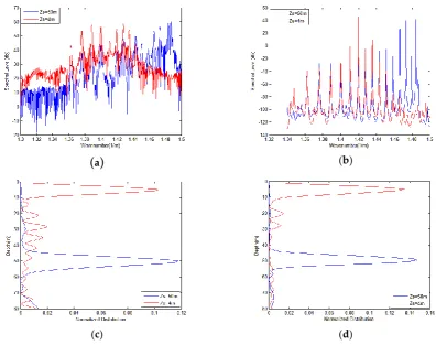
1. Range span is sufficient and SNR is high
219
The source moves 4990 m during the observation time. The SNR is 40 dB. From Figure 2a,b, the
220
peaks of wavenumber spectrum obtained by two methods are found to be clear. Therefore, we can
221
estimate wavenumbers accurately using the two methods under this simulation condition. Both
222
methods yield good depth estimation results as shown in Figure 2c,d. Comparing Figure 2c,d shows
223
that the sidelobes of the depth estimation in Figure 2d are smaller than those in Figure 2c, especially
224
for the shallow source. The number of mode wavenumbers estimated is 9 in Figure 2a and the
number is 11 in Figure 2b. The more mode wavenumbers are estimated correctly, the more
226
information can be taken into depth estimation. The performance of depth estimation can be
227
improved by increasing the number of mode wavenumbers estimated. Small sidelobes can also be
228
obtained. Thus, when the range span is sufficient and the SNR is high, the performance of depth
229
estimation using MMAR is slightly better than the performance of that using SAB.
230
(
a)
(b)(c) (d)
Figure 2. Comparison of SAB and MMAR in terms of source depth estimation by using simulated
231
pressure field data covering the range span of 4990 m with an SNR of 40 dB. (a) Mode wavenumber
232
extracted using the modified Hankel transform. (b) Wavenumber estimated using the AR model. (c)
233
Depth estimation using SAB. (d) Depth estimation using MMAR.
234
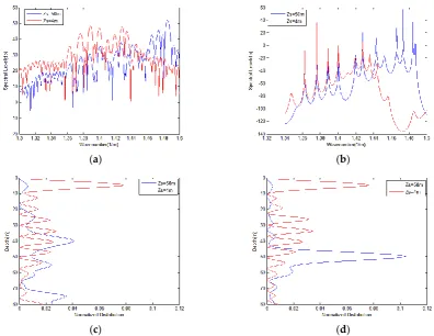
2. Range span is sufficient and SNR is low
235
In this simulation, the range span is 4990 m and the SNR is 5 dB. Only the deep source can be
236
estimated correctly as shown in Figure 3c. By contrast, the results in Figure 3d show good depth
237
estimation for the shallow and deep sources. SAB presents difficulty in estimating the mode
238
wavenumbers correctly as shown in Figure 3a. This difficulty is due to the influence of sidelobe
239
mask. MMAR based on AR model can reduce the influence of sidelobe mask. Thus, the spectral
240
peaks can be determined and the mode wavenumbers can be estimated accurately. When the range
241
span is sufficient and the SNR is low, the performance of depth estimation using MMAR improves
242
greatly compared with the performance of that using SAB.
(a) (b)
(c) (d)
Figure 3. Comparison of SAB and MMAR in terms of source depth estimation by using simulated
244
pressure field data covering the range span of 4990 m with an SNR of 5 dB. (a) Mode wavenumber
245
extracted using the modified Hankel transform of SAB. (b) Wavenumber estimated by the AR model
246
of MMAR. (c) Depth estimation using SAB. (d) Depth estimation using MMAR.
247
3. Range span is insufficient and SNR is high
248
The source moves 1990 m and the SNR is 40 dB in this simulation. Both methods can estimate
249
the shallow source depth effectively under this condition as shown in Figure 4c,d. SAB fails whereas
250
MMAR succeeds to estimate deep source depth. SAB mistakenly selects the sidelobe peaks as
251
estimations of the mode wavenumbers, and the false wavenumbers are shown in Figure 4a. By
252
contrast, the peaks of the main lobe can be extracted effectively and the miscarriage of justice can be
253
reduced using AR model. When the range span is insufficient and the SNR is high, the performance
254
of MMAR is better than the SAB. In particular, MMAR performs obviously better than SAB in terms
255
of estimation of deep source depth.
256
(a) (b)
(c) (d)
Figure 4.Comparison of SAB and MMAR in terms of source depth estimation by using simulated
257
pressure field data covering the range span of 4990 m with an SNR of 40 dB. (a) Mode wavenumber
extracted using the modified Hankel transform of SAB. (b) Wavenumber estimated by the AR model
259
of MMAR. (c) Depth estimation using SAB. (d) Depth estimation using MMAR.
260
The above mentioned analysis is based on the qualitative analysis of a single experiment, and
261
the following two types of algorithms are analyzed quantitatively from the statistical point of view.
262
In quantifying the estimated performance in an experiment, the correct index (CI) and output peak
263
sidelobe ratio (OPSLR) should be defined. CI can be expressed as
264
1 |
|
0 |
|
e s e s
z
z
g
CI
z
z
g
, (30)where
z
e is the result of source depth estimation andg
is the tolerance of the depth estimation.265
The OPSLR is defined as follows
266
'
max( ( )) max( ( ))
1
0
0
P z
P z
CI
OPSLR
CI
, (31)where
267
( )
( )
20 lg
max( ( ))
D z
P z
D z
, (32)min max
[
,
]
z
z
z
, (33)'
min max
[
,
s]
[
s,
]
z
z
z
g
z
g z
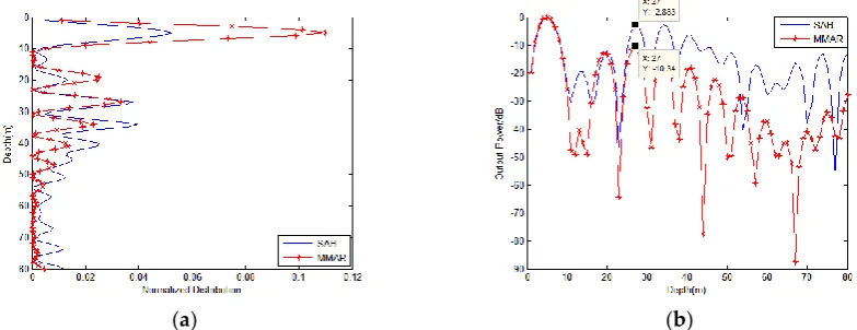
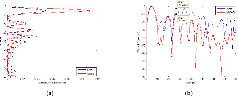
, (34)We adopt the condition in Figure 4 and consider only the shallow source to intuitively
268
understand the above-mentioned definition. The depth estimation results of the two algorithms are
269
shown in Figure 5a. In this case, the two methods can estimate the source depth correctly. The
270
OPSLR is marked for the two methods in Figure 5b. The OPSLR of SAB is 2.883 dB and that of
271
MMAR is 10.34 dB.
272
(a) (b)
Figure 5. Depth estimation. (a) Normalized depth ambiguity functions, (b) Output power at all
273
depths.
274
The correct probability (CP) and average peak sidelobe ratio (APSLR) are proposed to evaluate
275
the statistical performance of source depth estimation in multiple experiments. CP can be expressed
276
as
0
1 0
1
Nn
CP
CI
N
, and the APSLR is defined as0
1 0
1
Nn
APSLR
OPSLR
N
,where is the277
number of experiments in this simulation. The CP and APSLR with different range spans and SNRs
278
for source depth estimation is shown in Tables 1 and 2. The source depths are 4 and 50 m in Tables 1
279
and 2, respectively. From Tables 1 and 2, the performance of source depth estimation by MMAR is
found to better than the performance of that by SAB regardless of the source depth. The source
281
depth influences the algorithm as shown in Table 1 and 2. For effective comparison of performance
282
of two algorithms, the source depth is varied from 1 m to 80 m in Figure 6. The source moves 3990 m
283
and SNR is 20 dB. The similar regulation shown in Figure 6 can be found in other cases shown in
284
Tables 1 and 2. Figure 6 shows that MMAR presents an improvement in depth estimation for
285
different source depths compared with SAB.
286
Table 1. The results for the source depth of 4 m.
287
SNR(dB) Range(m) CP APSLR(dB)
SAB MMAR SAB MMAR
40
1990
0.772 1.000 1.440 10.737
30 0.598 1.000 1.121 9.788
20 0.338 0.998 1.018 8.201
15 0.260 0.898 0.841 6.856
20
2990 0.608 1.000 5.199 10.027
10 0.316 0.832 1.246 5.962
20
3990 0.934 1.000 7.924 10.804
10 0.422 0.942 1.604 8.012
10 4990 0.458 0.970 2.142 9.200
288
289
290
291
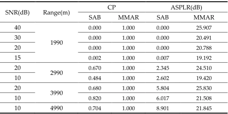
Table 2. The results for the source depth of 50 m.
292
SNR(dB) Range(m) CP ASPLR(dB)
SAB MMAR SAB MMAR
40
1990
0.000 1.000 0.000 25.907
30 0.000 1.000 0.000 20.491
20 0.000 1.000 0.000 20.788
15 0.002 1.000 0.007 19.192
20
2990 0.670 1.000 2.345 24.510
10 0.484 1.000 2.602 19.420
20
3990 0.680 1.000 5.804 25.830
10 0.820 1.000 6.017 21.508
10 4990 0.704 1.000 8.901 21.845
(a) (b)
Figure. 6. Depth estimation performance for the various source depths by using (a) CP and (b)
294
APSLR.
295
4.2. Selection of the HLA depth
296
After substituting Equation. (23) into Equation.(21), we can express the depth ambiguity
297
function as
298
2
2
2
1 ( )
( )
( )
1
m r
M
m m
m z
b
D z
z
, (35)From Equation. (35), the mode is found to not contribute to depth estimation when the HLA depth
299
r
z
coincides with the zero-crossing points of the mode depth function, that is ,
m( )
z
r0
. The300
performance is influenced not only by the range span and the SNR, but also by the HLA depth.
301
In determining the influence of the HLA depth, we consider the two above-mentioned sources
302
with a sufficient range span (4990 m) and high SNR. The HLA depth is varied from 1 m to 80 m to
303
obtain the performance of depth estimation for different HLA depths. The number of Monte Carlo
304
experiments is 500. Figure 7a shows the performance evaluated by CP with various HLA depths. For
305
the deep source, the HLA depth significantly influences the correction of depth estimation.
306
However, for the shallow source, CPs are all ones no matter where the HLA is located. This finding
307
means that the HLA depth slightly influences the correctness of depth estimation. Consequently, as
308
the source locates at different depths in the ocean, the HLA depth affects the source depth estimation
309
differently. The performance evaluated by APSLR is shown in Figure 7b. For the deep source, when
310
the HLA is located at 72 m, the largest value of APSLR occurs. For the shallow source, the APSLR
311
presents the largest value when the HLA depth is 36 m. We can conclude from the above-mentioned
312
observation that the most suitable HLA depth for depth estimation depends on the source depth.
313
Thus, performance for various source depths and HLA depths should be studied. On the basis of the
314
analysis present above, a suitable HLA depth span can be obtained for all source depths.
315
Figure 7. Depth estimation performance for shallow and deep sources from a single receiver at
316
various depth using (a) CP, and (b) APSLR.
317
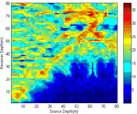
A common conclusion for HLA depth span is obtained after evaluating the performance for all
318
probable source depth. The performance evaluated by the APSLR for depth estimation under
319
various source and HLA depths is shown in Figure 8. As shown in the figure, when the HLA is
320
located near the water surface, the depth is difficult to be estimated correctly for some deep sources.
321
The optimum placement depth of HLA differs for dissimilar source depths. The general trend is that,
322
with the increasing of the source depth, the optimal placement depth of HLA also increases. In other
323
words, the optimum placement depth of HLA is determined by the source depth. Therefore, we
324
synthesize the depth estimation performance of the source with all possible depths and obtain the
325
HLA depth span that is suitable for depth estimation. The distribution of the source depth is
326
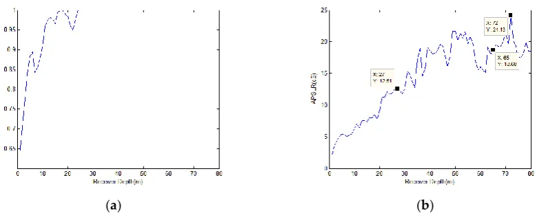
expressed by
p z
( )
, and is assumed to be uniform. The result of the integrated correct estimation327
probability (ICP) for different HLA depths is present in Figure 9. The figure shows that, when HLA
328
is located below 25 m, the correctness of depth estimation can be guaranteed for all possible source
329
depths. The integrated average peak sidelobe ratio (IAPSLR) as the placement depth of HLA
330
increases is shown in Figure 9b. IAPSLR can be calculated by
p z
( )
APSLR
. Synthesizing all331
possible source depths shows that, when the HLA depth is smaller than 30 m, the IAPSLR increases
332
with the placement depth of HLA. The general trend of the curve increases from 30 m to near the
333
boundaries, with an oscillatory plateau in the local part. Furthermore, the IAPSLR presents higher
334
value at this region than at the region of a source depth smaller than 30 m. When the HLA is located
335
at 72 m, the IAPSLR possesses the largest value. These curves are valid for the given environment
336
and frequency, but similar plateau can be observed with other downward-refracting SSPs.
337
Consequently, when the HLA is located below the transitional layer, we can obtain a satisfying
338
result of the source depth estimation. The conclusion is studied on the basis of the normal mode
339
theory.
340
341
Figure 8. The performance of the depth estimation is evaluated by APSLR. The figure shows APSLR
342
versus HLA and source depths.
(a) (b)
Figure 9. Curve for depth estimation performance with different HLA depths by using (a) ICP and
344
(b) IAPSLR.
345
Figure 10 shows the 10 modes excited by the 350 Hz narrowband signal, which is radiated by
346
the source located at 50 m. The mode excitation amplitudes are the function of depth. For example,
347
for the modes wherein the HLA is located at a range of 5010 m and a depth of 30 m, several mode
348
amplitudes (1th, 2nd, 8th, and 10th orders) is close to zero. The proposed method in this paper
349
estimates the wavenumber before depth estimation. The wavenumbers are difficult to estimate
350
when
m( )
z
r
m( )
z
s0
. The missing information degrades the performance of depth estimation.351
0 0.10.2 0 10 20 30 40 50 60 70 80
Mode 1
D
ep
th
(m
)
-0.2 0 0.2 Mode 2
-0.2 0 0.2 Mode 3
-0.2 0 0.2 Mode 4
-0.2 0 0.2 Mode 5
-0.2 0 0.2 Mode 6
-0.2 0 0.2 Mode 7
-0.2 0 0.2 Mode 8
-0.2 0 0.2 Mode 9
-0.2 0 0.2 Mode 10
352
Figure 10. Ten order normal modes excited by the 350 Hz cw. Several mode amplitudes (1th, 2nd,
353
8th, and 10th orders) is close to zero are shown in this figure.
354
We define the modes that contribute to the depth estimation as the modes with amplitudes
355
larger than
/ 2
. The number of modes that contribute to estimate source depth at various HLA356
depths is shown in Figure 11. Compared with other depths for HLA, 71 m and 72 m present a large
357
number of the modes that contribute to depth estimation. This conclusion is the same as that for
358
Figure 9b. In addition, the trend observed in Figure 11 is similar to that found in Figure 9b.
360
Figure 11. Number of modes that contribute to the source depth estimation at various receiver
361
depths.
362
The HLA is located at several depths wherein the IAPSLR is high whereas the number of modes
363
that contribute to depth estimation is small. For example, the number of modes is 11 when the HLA
364
is located at 65 m and the number is 12 when the HLA is located at 27 m (Figure 12). However,
365
IAPSLR at 37 m is high as shown in Figure 7b. The phenomenon can be explained by normal mode
366
theory. Figure 11 shows the amplitudes of modes when the HLA is located at 27 and 65 m. As shown
367
in Figure 10a, the lower order mode amplitudes are approximately zero when the HLA depth is 25
368
m. Figure 10b shows that the lower order mode amplitudes possess large values when the HLA
369
depth is 65 m. Using Equation. (21), the proposed depth estimation method is made equivalent to
370
weighted matched-mode depth estimation with coefficients of
0
2
sinh(
)
2
mr
m m
m m
R
e
c
k
. Figure371
13 shows that the weighting coefficients is monotonously decrease with the increase in mode order.
372
This finding indicates that the lower order modes provide high contribution for the depth
373
estimation. The number of modes is smaller but lower order mode amplitudes are higher when HLA
374
is located at 65 m than when HLA is located at 27 m. Consequently, the performance of depth
375
estimation when HLA is located at 65 m is good.
376
(a) (b)
Figure 12. Variation curve of mode amplitudes and mode orders of modes when HLA is located at
377
(a) 27m and (b) 65m.
379
Figure. 13. Weighting coefficients decrease with the increasing mode order.
380
On the basis of the discussion presented above, the performance of depth estimation is
381
determined by the number and the amplitudes of contributing modes, which are related with the
382
HLA depth. The combined contribution of both to depth estimation can be expressed as follows
383
1
,
M m m m
B
c X
, (36)1
( )
2
0
( )
2
m r m
m r
z
X
z
, (37)Figure 14 shows the contribution to depth estimation. Compared with Figure 11 and Figure 9b, a
384
higher similarity is obtained between Figure 14 and Figure 9b. In summary, when the HLA is located
385
below the transitional layer, the number of contributing modes is large and the lower order modes
386
are dominant. Therefore, the combined contribution is larger in this case. Thus, a good depth
387
estimation can be obtained when the HLA is located below the transitional layer.
388
389
Figure. 14. Contribution to depth estimation.
390
5. Conclusions
391
A matched-mode method based on AR using an HLA to estimate the moving source depth is
392
developed in this study. The modal wavenumber spectrum is obtained using generalized Hankel
393
transform with the data from the moving source. The mode amplitudes can be extracted by
394
combining the information based on AR modal wavenumber spectrum and the FT wavenumber
395
spectrum. The amplitudes contain the information of source depth. The source depth is estimated by
matching the mode estimation with the mode depth function calculated by the KRAKEN. The
397
method is robust for estimating source depth as a result of the robustness of its mode depth function.
398
The method proposed in this study is evaluated using the simulated data. For the data with a
399
small range span or low SNR, the proposed method can achieve source depth estimation with better
400
performance than SAB. The depth estimation performance is influenced not only by the range span
401
and SNR but also by the HLA depth. The selection for HLA depth is studied and the result is
402
explained by normal mode theory. In summary, when the HLA is located below the transitional
403
layer, good depth estimation result can be expected. This conclusion is valid for the shallow
404
waveguides with downward-refracting SSP.
405
Compared with that in SAB, the requirement of the moving source traveling range decreases in
406
proposed method. The proposed method can also be applied to the data with low SNR. However,
407
this method is limited because it assumes the source depth fixed during the observation time. The
408
effectiveness of this method degrades sharply, when the source depth varies rapidly. Thus,
409
additional work is needed for its future application in source depth tracking.
410
Acknowledgments: This work was supported by the National Key R&D Plan ( 2017YFC0306900 ), the National
411
Natural Science Foundation of China ( 11504064 and 61405041 ), the Technology of Basic Scientific Research
412
Project ( JSJL2016604B003 ), and the Open Fund for the National Laboratory for Marine Science and Technology
413
of QingDao.
414
Author Contributions: Zhang Yi-Feng and Liang Guo-Long conceived and designed the experiments; Zhang
415
Yi-Feng and Liang Guo-Long performed the experiments; Zhang Yi-Feng, Liang Guo-Long and Zou Nan
416
analyzed the data; Wang Jin-Jin contributed reagents/materials/analysis tools; Zhang Yi-Feng wrote the paper.
417
Conflicts of Interest: The authors declare no conflict of interest.
References
420
1. Baggeroer, A. B.; Kuperman, W. A.; Mikhalevsky, P. N. An overview of matched field methods in ocean
421
acoustics. IEEE J. Ocean. Eng. 1993,18 (4), 401-424, doi: 10.1109/48.262292.
422
2. Wang, Q; Wang, Y. M.; Zhu G. L. Matched field processing based on least squares with a small aperture
423
hydrophone array. Sensors2017, 17, 71, doi: 10.3390/s17010071.
424
3. Yang, T. C., A method of range and depth estimation by modal decomposition. The J. Acoust. Soc. Am. 1987,
425
82 (5), 1736-1745, doi: 10.1121/1.395825.
426
4. Gall, Y. L.; Socheleau, F. X.; Bonnel, J., Matched-Field Processing Performance Under the Stochastic and
427
Deterministic Signal Models. IEEE Trans. Signal Process. 2014, 62 (22), 5825-5838, doi:
428
10.1109/TSP.2014.2360818.
429
5. Jesus, S. M.; Porter, M. B.; Stephan, Y.; Demoulin, X.; Rodriguez, O. C.; Coelho, E. M. M. F., Single
430
hydrophone source localization. IEEE J. Ocean. Eng. 2002,25 (3), 337-346, doi: 10.1109/48.855379.
431
6. Suppappola, S. B.; Harrison, B. F., Experimental matched-field localization results using a short vertical
432
array and mid-frequency signals in shallow water. IEEE J. Ocean. Eng. 2004, 29 (2), 511-523, doi:
433
10.1109/JOE.2004.826896.
434
7. Yang, T. C., Source depth estimation based on synthetic aperture beamfoming for a moving source. J.
435
Acoust. Soc. Am. 2015, 138 (3), 1678-1686, doi: 10.1121/1.4929748.
436
8. Rui, D.; Kun-De, Y.; Yuan-Liang, M.; Bo, L., A reliable acoustic path: Physical properties and a source
437
localization method. Chin. Phys. B2012,21 (12), 276-289, doi: 10.1088/1674-1056/21/12/124301.
438
9. O., B. N.; A., B. P.; A., R. J.; W., S. P.; S., H. W.; L., D. S. G.; J., M. J., Source localization with broad-band
439
matched-field processing in shallow water. IEEE J. Ocean. Eng. 1996,21, 402, doi: 10.1109/48.544051.
440
10. Forero, P. A.; Baxley, P. A.; Straatemeier, L., A Multitask Learning Framework for Broadband
441
Source-Location Mapping Using Passive Sonar. IEEE Trans. Signal Process. 2015,63 (14), 3599-3614, doi:
442
10.1109/TSP.2015.2432747.
443
11. Bonnel, J.; Caporale, S.; Thode, A., Waveguide mode amplitude estimation using warping and phase
444
compensation. J. Acoust. Soc. Am. 2017,141 (3), 2243-2255, doi: 10.1121/1.4979057.
445
12. Yang, T. C.; Xu W., Data-based depth estimation of an incoming autonomous underwater vehicle. J.
446
Acoust. Soc. Am. 2016, 140 (4), EL302-EL306, doi: 10.1121/1.4964640.
447
13. Yang, T. C., Data-based matched-mode source localization for a moving source. J. Acoust. Soc. Am. 2014,
448
135 (3), 1218-1230, doi: 10.1121/1.4863270.
449
14. Liu, H. W; Li, B. Q.; Yuan, X. B.; Zhou, Q. W.; Huang, J. C., A robust real time direction-of-arrival
450
estimation method for sequential movement events of vehicles. Sensors 2018, 18, 992,
451
doi:10.3390/s18040992.
452
15. Frisk, G. V.; Lynch, J. F., Shallow water waveguide characterization using the Hankel transform. J. Acoust.
453
Soc. Am. 1984,76 (1), 205-216, doi: 10.1121/1.391098.
454
16. Sarkar, T. K.; Pereira, O., Using the matrix pencil method to estimate the parameters of a sum of complex
455
exponentials. IEEE Antennas Propag. Mag. 1995,37 (1), 48-55, doi: 10.1109/74.370583.
456
17. Roux, P.; Cassereau, D.; Roux, A., A high-resolution algorithm for wave number estimation using
457
holographic array processing. J. Acoust. Soc. Am. 2004,115 (3), 1059-1067, doi: 10.1121/1.1648321.