Bias reduction for TDOA localization in the presence of receiver position errors and synchronization clock bias

R E S E A R C H

Open Access

Bias reduction for TDOA localization in the

presence of receiver position errors and

synchronization clock bias

Xin Chen

, Ding Wang

, Jiexin Yin

, Changgui Jia

and Ying Wu

Abstract

Time difference of arrival (TDOA) localization does not require time stamping of the source signal and is playing an increasingly important role in passive location. In addition to measurement noise, receiver position errors and synchronization clock bias are two important factors affecting the performance of TDOA positioning. This paper proposes a bias-reduced solution for passive source localization using TDOA measurements in the presence of receiver position errors and synchronization clock bias. Like the original two-step weighted least-squares solution, the new technique has two stages. In the first stage, the proposed method expands the parameter space in the weighted least-squares (WLS) formulation and imposes a quadratic constraint to suppress the bias. In the second stage, an effective WLS estimator is given to reduce the bias generated by nonlinear operations. With the aid of second-order error analysis, theoretical biases for the original solution and proposed bias-reduced solution are derived, and it is proved that the proposed bias-reduced method can achieve the Cramér–Rao lower bound performance under moderate Gaussian noise, while having smaller bias than the original algorithm. Simulation results exhibit smaller estimation bias and better robustness for all estimates, including those of the source position, refined receiver positions, and clock bias vector, when the measurement noise or receiver position error increases.

Keywords:Passive location, Bias reduction, Synchronization clock bias, Receiver position error, Time difference of arrival

1 Introduction

The problem of passive localization has in recent decades been of wide concern and studied intensely by scholars in many fields, such as passive radar [1–3], wireless commu-nication [4–6], sensor networks [7, 8], and underwater

acoustics [9, 10]. Most localization techniques use

two-step processing, in which the positioning parameters are first extracted (or estimated) and the source position is then determined according to these estimated parameters. The positioning parameters are nonlinear functions with respect to the source position and are usually the received signal strength (RSS) [11–16], gain ratios of arrival [17, 18], time of arrival (TOA) [19,20], time difference of

ar-rival (TDOA) [21–27], frequency difference of arrival

(FDOA) [28, 29], and angle of arrival (AOA) [30, 31].

Among these, TDOA localization is perhaps one of the most frequently used schemes, because it has superior po-sitioning performance and does not require the time stamp of the source signal. This paper focuses on the localization of a single source using TDOA measurements obtained at spatially separated receivers.

A number of TDOA localization algorithms have been developed during the past few decades. Many methods are iterative owing to the highly nonlinear relationship be-tween unknowns and TDOA measurements. The Taylor series method begins with an initial guess and uses local linear least-sum-square-error corrections to improve the estimation accuracy in each iteration [24, 32]. The con-strained total least-squares (CTLS) algorithm [22] has been proposed and the Newton iteration applied to esti-mate the source position. These methods have high localization accuracy in the case of a good initial guess close to the true value; however, such prior information of the initial guess is not readily available in practice. It is therefore difficult to guarantee convergence. To overcome * Correspondence:[email protected]

1_{National Digital Switching System Engineering & Technology Research} Center, Zhengzhou 450002, People_’s Republic of China

2_{Zhengzhou Information Science and Technology Institute, Zhengzhou,} Henan 450002, People’s Republic of China

the drawback of iterative algorithms, several closed-form methods using TDOAs have been proposed, such as the total least-squares (TLS) algorithm [25] and two-step weighted least-squares (TSWLS) positioning algorithm [21, 29, 33]. It has been shown both theoretically and by simulation that the above methods can achieve the

Cramér–Rao lower bound (CRLB) under small Gaussian

noise levels. Obviously, compared with iterative algo-rithms, closed-form methods are more attractive because they do not require an initial guess and avoid the problem of divergence. We concentrate on the closed-form method in this paper.

Most existing TDOA localization algorithms require the receiver locations to be accurately known and the ceivers to be strictly synchronized in sampling the re-ceived signals, but these are unlikely to be satisfied in practice. As examples, receivers (or sensors) are fixed on vessels or aircraft or they are randomly arranged in a cer-tain region, which results in the true receiver positions to be compromised by receiver position errors. In addition, when the receivers are far away from each other, it is diffi-cult to achieve strict clock synchronization for all re-ceivers. Many studies have shown that both the receiver position errors and synchronization clock bias play im-portant roles in TDOA localization because they

deterior-ate the positioning accuracy [29, 32, 34]. Indeed, the

problem of jointly suppressing the receiver position error and synchronization clock bias has been intensively stud-ied in recent years. A joint synchronization and source localization algorithm with erroneous receiver positions has been proposed [35], where the clock bias is assumed to be known with random errors, whereas such prior in-formation with respect to synchronization clock bias is not available in practice. To overcome this drawback, a novel closed-form solution method, in which the clock bias is considered a deterministic parameter, has been de-veloped and the algebraic solutions of the source location, receiver positions, and synchronization offsets were se-quentially obtained [36]. This method is practical and ef-fective and not only jointly suppresses receiver position error and synchronization clock bias but also obtains the CRLB under low noise levels.

However, the original algorithm proposed in [36] has a drawback in that the bias of estimates is too large owing to the noise correlation between the regressor and regressand in the weighted least-squares (WLS) formulation and some nonlinear operations. Especially when the noise level is high or the localization geometry is not good enough, the bias becomes large and seriously affects the localization per-formance. Moreover, in some modern applications, we can obtain multiple independent measurements in a short time period. The localization performance can be improved by averaging these estimates from multiple independent mea-surements. Nevertheless, this operation only reduces the

variance and not the bias. In tracking applications, the bias problem remains because the measurements made at dif-ferent instants are coherent [37]. It is therefore necessary to reduce the bias to improve the localization performance. Over the years, many studies have reduced the bias of an estimator using TDOAs [38–45]. Two methods of reducing the bias of the closed-form solution using TDOAs have been proposed [38], but the receiver position errors and synchronization clock bias were not taken into account. One study [39] proposed a bias-reduced method for a two-sensor (or two-receiver) positioning system based on TDOA and AOA measurements in the presence of sensor errors. The simulation validates the availability of the pro-posed method. Moreover, an improved algebraic solution employing new stage-2 processing for the TDOA with sen-sor position errors has been proposed [40]. Simulation re-sults show lower estimation bias; however, this method only improves the stage-2 processing, and the bias intro-duced in stage 1 needs to be further reintro-duced.

Inspired by previous works [38–45], this paper

pro-poses a bias-reduced method of reducing the bias of es-timates from [36] using TDOAs in the presence of receiver position errors and synchronization clock bias. The study begins with a bias analysis for the original TSWLS solution. Results show that the bias of the ori-ginal algorithm mainly comes from the noise correlation of the WLS problem in the first stage and the nonlinear operations in the second stage. On this basis, the proposed method introduces an augmented matrix and imposes a quadratic constraint in the first stage. Gener-alized singular value decomposition (GSVD) is then used to obtain the stage-1 solution. A new WLS estimator is designed to correct the stage-2 solution and avoid the use of nonlinear operations. Moreover, this paper derives a theoretical bias for the proposed method, and perform-ance analysis indicates that the proposed bias-reduced method effectively reduces bias without increasing the values in the covariance matrix. Finally, simulation re-sults verify the validity of the theoretical derivation and the superiority of the proposed method.

Compared with the previous works related to bias re-duction, the major contributions of this paper are as follows.

1. Different from most existing bias reduction methods [38–45], the proposed method considers both receiver position errors and synchronization clock bias.

2. Through second-order error analysis, [38] investi-gated the bias of the classical TSWLS method [33]. The present paper extends the bias analysis using a more realistic positioning model [36], which con-siders both receiver position errors and

3. All previous studies [38–45] aim at reducing the bias of the source position. We develop a bias-reduced method that effectively reduces not only the bias of the source position but also the bias of refined re-ceiver positions and estimated clock bias vector. 4. Previous works [43,44] reduced the bias, but the

estimation variance was higher than that of the original solution. The method proposed in this paper reduces the bias of the solution without increasing the root mean square error (RMSE). 5. The performance of the proposed bias-reduced

method is theoretically derived and it is shown that the proposed bias-reduced method effectively reduces the bias without increasing the estimation variance.

The remainder of this paper is organized as follows.

The measurement model in the presence of

synchronization clock bias and the original TSWLS

solu-tion are described in Secsolu-tion 2. Section 3 presents the

performance analysis for the original TSWLS solution. Section4develops a bias-reduced solution. In Section5, the theoretical bias for the proposed method is derived with the aid of second-order error analysis. Simulation results are presented in Section 6while conclusions are

presented in Section 7. The main notations used in this

paper are listed in Table1.

2 Measurement model and original TSWLS method

2.1 TDOA measurement model in the presence of receiver position errors and synchronization clock bias

Consider a three-dimensional localization scenario, in

which M stationary receivers at so

m;m¼1;2;⋯;M

receive the signal emitted from a point source whose

un-known location is to be determined, denoted by uo.

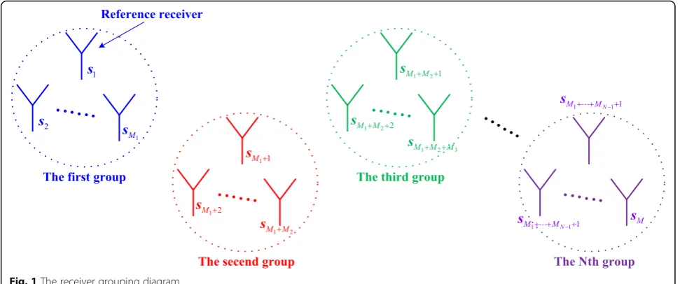
Similar to [36], receivers are separated into N groups.

Within each group, the receivers share a common local clock. However, the local clocks for different receiver groups are not the same, and there are thus clock offsets

among the groups. Assuming that the first n receiver

groups haveMnreceivers, there areMn−Mn−1receivers

in the nth group, where M0= 0 and MN=M. The

re-ceiver grouping diagram is shown as Fig.1.

The clock offset of groupnwith respect to group 1 is de-noted asτn,n= 1, 2,…,N, whereτ1= 0. The first receiver is chosen as the reference, and the TDOA measurement from the receiver pairmand 1 is denoted astm1. The relationship with the range difference of arrival (RDOA) measurement rm1isrm1=c⋅tm1, wherecis the signal propagation speed. For convenience, we directly discuss the RDOAs in the fol-lowing derivation. The RDOAs can be modeled as

rm1¼ro_m1þδnþΔrm1; m¼Mn−1þ1;Mn−1þ2;…;

Mn;n¼1;2;…;N;

ð1Þ

where Δrm1 represents the measurement noise, δn=

cτn(δ1= 0), and the true valuero_m1 is

rom1¼‖uo−som‖−‖uo−so1‖; m¼2;3;⋯M: ð2Þ

Rewriting (1) in vector format, we attain

r¼ro_{þΓδþΔr; : ð3Þ}

where vectorsr= [r21,r31,⋯,rM1]T, ro¼ ½ro21;ro31;⋯;roM1 T

and Δr= [Δr21,Δr31,⋯,ΔrM1]T comprise all measure-ments, true value, and measurement noise, respect-ively. δ= [δ2,δ3,⋯,δN]T is the clock bias vector,

which is modeled as being deterministic. Γ¼ ½

OðM1−1ÞðN−1Þ

blkdiag½1M21 1M31 ⋯ 1MN1∈R

ðM−1ÞðN−1Þ _{is a column}

full-rank matrix; i.e., rank[Γ] =N−1. Assume that the

RDOA noise vector Δr follows a zero-mean Gaussian

distribution with covariance matrix Q1.

Similar to [21, 23, 24], the receiver positions are not known exactly. The available receiver position for re-ceivermis expressed as

sm¼somþΔsm; m¼1;2;⋯;M; ð4Þ

where Δsm represents random errors having covariance

matrixQ_sm. Rewriting (4) in vector format, we have

s¼so_{þΔs; ð5Þ}

wheres¼ ½sT₁;s₂T;⋯;sT_MT, so¼ ½soT₁ ;soT₂ ;⋯;soT_MT and Δ s¼ ½ΔsT

1;ΔsT2;⋯;ΔsTM T

is the receiver position error vector, which is assumed to have a zero mean and be Table 1Mathematical notation

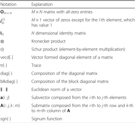
Notation Explanation

OM×N M×Nmatrix with all-zero entries

iðlÞ

M M× 1 vector of zeros except for thel-th element, which has value 1

IN Ndimensional identity matrix

⊗ Kronecker product

⊙ Schur product (element-by-element multiplication) vecd[⋅] Vector formed diagonal element of a matrix

tr{⋅} Trace

diag{⋅} Composition of the diagonal matrix

blkdiag{⋅} Composition of the block diagonal matrix

‖⋅‖ Euclidean norm of a vector

a(i:j) Subvector composed from thei-th toj-th elements

A(i:j,k:m) Submatrix composed from thei-th toj-th row andk-th tom-th column ofA

Gaussian distributed with covariance matrixQ2¼blkdiag fQs1;Qs2;⋯;QsMg. Measurement noise Δr and receiver position errorΔsare independent of each other.

The localization problem is to obtain an estimate of uo_,so_{, andδ}o_{as accurately as possible using the available} measurementsrand the receiver positionss.

Remark 1: In practice, the clock-offset grouping can be implemented according to the distance between re-ceivers. When the receivers are close to each other, synchronization is easily performed using a single piece of hardware with multichannel acquisition capabilities. If the receivers are far away, synchronous sampling will be a big challenge [36]. Therefore, receivers that are rela-tively close to each other are put into the same group.

2.2 Original TSWLS method

For the TDOA positioning problem in the presence of receiver position errors and synchronization clock bias, [36] proposed a novel computationally efficient method, in which the algebraic solutions of the source location, receiver positions, and synchronization clock bias are es-timated sequentially. The method has two stages for

tar-get location estimation. The first stage introduces _N

nuisance variables doMn−1þ1¼‖uo−sMn−1þ1‖; n¼1;2;⋯ N to get the initial solution for the source location and these nuisance variables. In the second stage, the rela-tionship between uo and doMn−1þ1 is used to improve

the precision of the estimated source position. The final estimate of the source location is obtained by re-mapping the stage-2 solution. Moreover, the solution

is valid when M−N≥N+ 3 (i.e., the number of

equa-tions is greater than or equal to the number of un-knowns). The process of the algorithm is summarized in the following, and details of the derivation can be found in the literature [36].

Stage 1: stage-1 solution, consisting of the estimated target loca-tion and nuisance variables, and

G1¼−2

The compositions in (9) are expressed as

A¼blkdiagfZ1;Z2;⋯;ZNg

Note that the true receiver location so_m in B1 can be

replaced by the noisy version sm. Additionally, both

B1 and D1 in W1 contain the true source locations,

which are unknown. To overcome this problem, W1

is first set to an identity matrix, and an initial solu-tion is obtained from (6), say φ^₁, from which an

ap-proximate W1 is obtained, thereby getting the stage-1

solution. The error due to the approximation of W1

is negligible [36].

where φ2=u⊙u represents the stage-2 solution,

which is equal to the Schur product of the target loca-tion estimate, and

The final source position solution is

u¼Π ffiffiffiffiffiffiffiffiffiffiffiffiffiffiffiffiffiffiφ2ð1:3Þ

q

; ð16Þ

where

Π¼ diag sgnf ðφ₁ð1:3ÞÞg: ð17Þ

According to [38], the source position estimate has ap-preciable bias for the classical TSWLS method [33] when the noise level is high or the localization geometry is poor. It can therefore be judged that the bias of the

original TSWLS algorithm [36] under receiver position errors and synchronization clock bias is also large. To solve this problem, the present paper designs a new reduced-bias estimator for this scenario. It was previ-ously necessary to derive the expression of the bias for the original TSWLS algorithm.

3 Performance analysis of the original TSWLS method

This section analyzes the performance of the original TSWLS solution using second-order error analysis. Two basic assumptions are made in our analysis. (1) The noise level is not high and higher second-order error terms can thus be ignored. (2) The source is sufficiently far from each receiver for the performance

loss due to the approximation of W1 to be negligible.

3.1 Bias analysis forφ1

Subtracting the true value φo₁ from both sides of (6), the estimation error inφ1can be expressed as.

Δφ1¼ GT1W1G1

and ignoring the higher second-order error terms, h1−

Note that (19) uses the approximationro

According to the Neumann expansion [46], we have

U−1

1 ≈ I−Uo−1 1ΔU1

Uo−1

1 : ð24Þ

Substituting (19), (22), and (24) into (18) yields

Δφ1¼ Uo1−1−U1o−1ΔU1Uo1−1

ation for (25) yields

E½Δφ1 ¼H1vecd AQ1AT

(A.7) in Appendix A. The first two components H

1vec-d[AQ1AT] and H1Evecd[Q2] come from second-order error terms due to the square operations for the measure-ments and receiver positions inh1, respectively. The third component comes from the second-order error termΔsT_m PmΔsm due to the Taylor series expansion for doMn−1þ1. The remaining components come from measurement noise and receiver position errors in regressorG1

3.2 Bias analysis forφ2

Subtracting the true value φo

2 from both sides of (12)

yields

h2−G2φo2¼Bo2Δφ1þΔφ1⊙Δφ1; ð28Þ version becauseG1andB2in it contain noise. According to the definitions ofB2in (15) andBo₂ (29), we haveΔB2

Substituting (23) and (30) into (14), and ignoring the higher first-order error terms yields

W2¼ Bo2−1−B2o−1ΔB2Bo2−1

Applying the Neumann expansion [46] again, we have U−1

2 ≈Uo2−1−U2o−1ΔU2Uo2−1. Substituting (28) and (32) into (27) and ignoring the higher second-order error terms yields

Hence, taking the expectation for (34) yields

E½Δφ₂ ¼H2 Bo2E½Δφ1 þvecd E Δφ1Δφ1T from the bias in the stage-1 solution. The second com-ponent H2vecd[E[Δφ1Δφ1T]] is from the square

oper-ation for φ1 in h2, while the remaining components

come from measurement noise and receiver position er-rors inG1andΔφ1inB2.

3.3 Bias analysis for u

According to (12), and we express φ₂¼φo yields the bias inuas

4 Proposed bias-reduced method

The proposed bias-reduced technique has two stages as follows.

4.1 Stage 1

According to the analysis in Section 3.1, the bias in the stage-1 solutionφ1mainly comes from the noise correl-ation between the regressorG1and regressandh1in the WLS formulation. The main purpose of this stage is to find a betterφ1with small bias. The main idea is intro-ducing an augmented matrix and imposing a quadratic constraint, so that the expectation of the cost function reaches a minimum value when the unknown is equal to the true value.

From [36], we obtain the noise matrix equation in the first stage as ε1¼B1AΔrþD1Δs¼h1−G1φo1;whereφo1

is the true value of φ1. The cost function of this WLS

problem is

, (42) can be rewritten as

J ¼vTAT1W1A1v: ð43Þ

A1contains measurement noise and receiver position

errors, and can be decomposed as

A1¼Ao1þΔA1: ð44Þ

According to the definition ofA1, after subtracting the true value Ao₁¼ ½−G₁o;ho₁ , and ignoring the second-order noise terms, we have

ΔA1¼2 A2Δ~s;ΛðINðAΔrÞÞ;B~1AΔrþC1Δs

Substituting (44) into (43) yields the cost function

J ¼vTAoT1 W1Ao1vþv T_ΔAT

1W1ΔA1vþ2vTΔAT1W1Ao1v: ð48Þ

Taking the expectation yields

E½ ¼J vTAoT1 W1A1ovþvTE ΔAT1W1ΔA1

v: ð49Þ

The third term in (48) vanishes in the expectation

be-cause ΔA1 is zero-mean. When we minimize E[J] with

respect to v, the second term on the right-hand side of (49) is the cause of bias, because the first term is zero at v=vo (Ao₁vo_{¼0). If we impose a constraint that makes} the second term constant, E[J] will reach minimum value atv=vo. We thus findvusing

min vTAT₁W1A1v s:t: vTΩv¼k; ð50Þ

where Ω¼E½ΔAT₁W1ΔA1, and the constant k can be any value. We can use the Lagrange multiplier method to solve the constrained minimization problem (50). Using Lagrange multiplierλ, we obtain the auxiliary cost function vT_AT

1W1A1vþλðk−vTΩvÞ. Taking the deriva-tive with respect tov, we have

AT 1W1A1

v¼λΩv: ð51Þ

Premultiplying both sides of (51) by vTand using the equality constraintvTΩv=k, we attain

λ¼vT _AT 1W1A1

v=k: ð52Þ

We here find the above equation has the same form as the objective function (50). Hence, we only need to

minimize λ. According to (51), λ is the generalized

eigenvalue of the pair ðAT₁W1A1;ΩÞ. The estimate vis therefore the generalized eigenvector that corresponds to the minimum generalized eigenvalue for the pair ðAT₁ W1A1;ΩÞ. The stage-1 solution can be expressed as

φ1¼vð1:3þNÞ=vð4þNÞ: ð53Þ

We now derive the formula for Ω. Substituting (45)

Ω2;3¼E ðΛðINðAΔrÞÞÞTW1B~1AΔr

in (60) depend on B~1, which is unknown. To facilitate implementation, the true values in B~1 are replaced by the measurements, and the performance loss due this approximation is negligible.

Remark 3: The weight matrixW1is also approximated

through the procedure described below (11). The loss due to the approximation is negligible when the source is away from each receiver. The proposed bias-reduced method is thus more suitable for distant source localization.

4.2 Stage 2

The performance analysis in Subsections 3.2 and 3.3

reveals that some nonlinear operations, including the squaring and square root operations in stage 2 of the original method increase the estimation bias. To re-duce the use of these nonlinear operations, a new version of stage 2 is developed in this subsection. The main idea is of this stage is to estimate the estimation

error of the stage-1 solution ^u¼φ₁ð1:3Þ, and cor-rect the solution u^ using this estimation error.

For N nuisance variables, we expand them around ^u

and retaining up to the linear term ofΔu^,

proximately zero-mean. Following Sorenson’s method

[47], we have

031¼Δ^u−Δ^u: ð64Þ

Combining (64) and the second equation in (63) gives

Δφ1¼

It is worth emphasizing that Δφ1 represents the esti-mation error of the stage-1 solution.

Then, using the WLS formulation, the desired estimate ofΔu^can be obtain as The final solution can be obtained by subtracting φ~₂ from the stage-1 solution^u:

u¼u^−φ~2: ð68Þ

The proposed bias-reduced method using TDOAs in

the presence of receiver position errors and

synchronization clock bias is summarized in Algorithm 1.

Remark 4: Although the proposed bias-reduced method only improves the source position solution, it can still reduce the bias for subsequent estimates

including receiver positions and the synchronization clock bias vector.

4.3 Complexity analysis

This subsection investigates the computational complex-ity of the proposed bias-reduced method in terms of the number of multiplications. The numerical complexity is

summarized in Table2.

We next compare the computational complexity of the proposed bias-reduced method with that of the ori-ginal TSWLS method [36]. Through analysis, the total computational complexity of original TSWLS method is O((M−N)3) +O((N+l)3) +O(l3) + (M−N)M2l2+ (M −N)2Ml+ 2(M−N)2(M−1) + (M−N)(M−1)2+ (M− N)3+ 3(N+l)⋅(M−N)2+ 3(N+l)2(M−N) + (N+l)(M −N) + 2(N+l)3+ 2l2(N+l) + 2l(N+l)2+l(N+l) + 2Nl2

+Ml+M+l. The main computational complexities of

the proposed method and the original TSWLS algo-rithm are respectively O((M−N)3) +O((N+l+ 1)3) + O(l3) andO((M−N)3) +O((N+l)3) +O(l3). By compari-son, we find that the computational complexity of the

proposed bias-reduced method is comparable to

(slightly larger than) that of the original TSWLS algorithm.

5 Performance analysis of the proposed bias-reduced method

This section analyzes the theoretical performance of the proposed bias-reduced method. The bias and covariance matrix of the solution are derived according to second-order error analysis. The same two assumptions described in Section3are made.

5.1 Stage 1

We denote the solution of (50) asv. The stage-1 solution of the proposed method is φ1=v(1 : 3 +N)/v(4 +N).. The equation errorA1vcan be expressed as

A1v¼½−G1;h1 φ₁1 The optimization problem (50) is therefore equivalent to

A the same partition. Substituting (72) and (73) into (71) yields ½Go₁TW1Go1;−G1oTW1ðh1−ΔG1φ1Þv¼0. Dividing

With some algebraic manipulations, we have the equality relationship

whereH1is defined below (25). When the noise level is small,Δφ1can be expressed as

According to (A.1)–(A.7) in Appendix A, the bias

E[Δφ1] can be obtained as Table 2Complexity of proposed method

Computational unit

Complexity for each unit Total computational complexity

A1 M−N+Ml OððM−NÞ3Þ þOððNþlþ1Þ3Þ þOðl3Þ þ ðN2þ2Nþ1Þ

E½Δφ1 ¼H1vecdAQ1AT

If we keep the first-order error terms, multiplying (78) by its transpose and taking the expectation yields the co-variance matrix

Subtracting the true valueφ~o₂from both sides of (67) yields

Δφ~2¼ G~ measurement noise and receiver position error. Using (23) and the definition ofW~2used for (67), we have

Adopting the Neumann expansion [46], we have the approximation U~−₂1≈U~o₂−1−U~o₂−1ΔU~2U~

o−1

2 . Substituting

(82) and (83) into (81) and ignoring the higher second-order error terms yields

Δφ~2¼ U~

some algebraic manipulations, we have

~ ing the expectation for (85) and using (86) yields

E½Δφ~₂ ¼H~2B~2E½Δφ1 þU~

If we keep the first-order error terms, multiplying (85) by its transpose and taking the expectation yields the co-variance matrix ofφ~₂as

is derived in (80).

The estimation error in the final solution u can be

expressed as variance matrix ofuare therefore

E½Δu ¼−E½Δφ~₂

respectively. We now state the following equation that

is proved in AppendixB:

EΔuΔuT¼ G~T₂W~o₂G~2

The following conclusions can be drawn from the above performance analysis.

find that the proposed method removes the bias terms (A.4) and (A.5) generated by the noise correlation betweenG1andh1. According to the discussion following Eq. (26), the proposed method does not completely decorrelate the noise fromG1 andh1, and retains the small bias terms (A.6) and (A.7). Moreover, the removed terms represent most of the bias caused by the noise correlation between G1andh1.

2. The bias of final source position estimate is obtained by combining (79) and (90). Compared with the bias of the original algorithm (41), the bias expression in (90) is more concise because our method avoids the use of nonlinear operations in stage 2, including squaring and square root operations.

3. From (92), we see that the proposed method has the same covariance matrix as the original algorithm, which indicates that under moderate noise, the proposed bias-reduced method can achieve the CRLB like the original algorithm. The proposed method therefore reduces the bias of the solution without in-creasing values in the covariance matrix.

Remark 5: For the proposed bias-reduced method, the main idea in stage 1 is introducing an augmented matrix and imposing a quadratic constraint, so that the

expectation of the cost function E[J] (ideal bias) reaches a minimum value of zero atv=vo. Stage-2 designs an ef-fective WLS estimator with which to further reduce the bias. The remaining parts of the bias are therefore negli-gible compared with the removed parts of the bias. This is verified in the following simulation.

6 Simulation results and discussion

This section conducts several simulation experiments to verify the superiority of the proposed bias-reduced algo-rithm and the validity of the theoretical derivation. We

conduct L= 10000 Monte Carlo (MC) experiments and

evaluate the localization accuracy in terms of the RMSE,

RMSEðuÞ ¼

ffiffiffiffiffiffiffiffiffiffiffiffiffiffiffiffiffiffiffiffiffiffiffiffiffiffiffiffiffiffiffi 1

L P l¼1 L

k^uðlÞ_−uok2; r

and the bias, biasðuÞ ¼ k P

l¼1 L

ðu^ðlÞ_−uo_{Þk=L. Note that the RMSE and bias for the}

re-ceiver position and clock bias vector are defined in the same manner.

6.1 Comparison of localization performance with the original TSWLS method

The experiment considers a three-dimensional

localization scenario. We assume there are 17 available

receivers having the positions listed in Table 3. The

source is placed atuo= [15, 16, 17]Tkm. The localization Table 3Location of the receivers (units: m)

Receiver no. 1 2 3 4 5 6 7 8 9 10

xo

i −1000 −1600 −1800 −1700 −2100 −2300 1900 2000 1700 2100

yo

i 1000 2100 1800 1600 1700 1500 −1400 −1900 −1800 −1600

zo

i 1000 1900 1600 1900 2000 2200 1300 1500 1900 1700

Receiver no. 11 12 13 14 15 16 17

xo

i 1500 2200 1900 −1200 −1400 −1700 −2300

yo

i 1600 1800 1700 −1500 −1700 1900 2100

zo

i −1700 −2300 −2000 1900 2100 −1800 −1700

Group 5

Group 2

Group 1

u

1

s

s

4

s

s

s

7

s

s

9

s

s

16

s

s

3

s

geometry is shown in Fig. 2. Moreover, the receivers are separated into five groups according to differences in local clocks; group 1 comprises receivers 1–6, group 2

comprises receivers 7–10, group 3 comprises receivers

11–13, group 4 comprises receivers 14–15, and group 5

comprises receivers 16–17. The following simulation

results show the RMSEs and biases for the proposed

bias-reduced method (see Section 4) and the original

TSWLS method [36]. To verify the theoretical analysis presented in the text, the following graphs also show the theoretical bias curves of the two algorithms (see

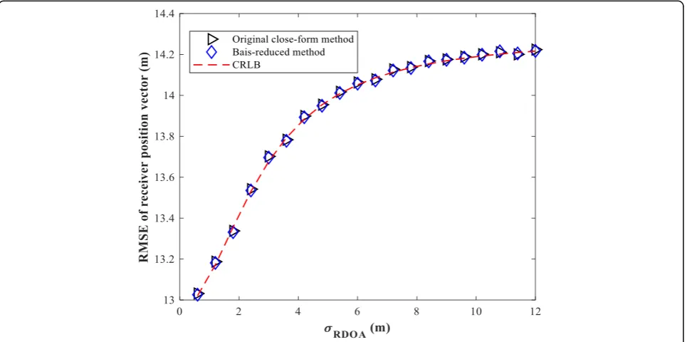
Sections3and5) and the corresponding CRLBs.

Fig. 3The RMSE of the source position as measurement noise varies

Assume that the RDOAs and receiver positions are contaminated by zero-mean Gaussian noise with covari-ance matrices Q1¼σ2RDOA~I and Q2¼σ2sI, where ~Ihas diagonal elements equal to unity and off-diagonal

ele-ments of 0.5. σRDOA and σs respectively represent the

noise level of the RDOAs and receiver positions. We

first set the clock bias vectorδ= [40 60 80 100]T m

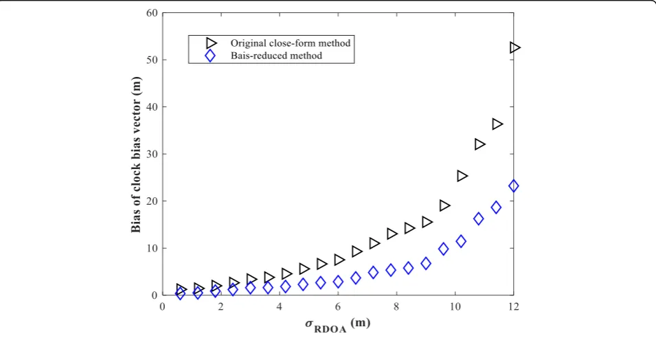
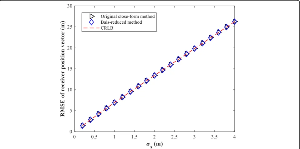
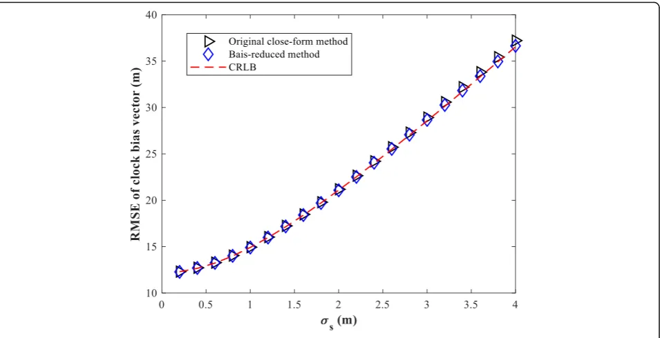
and the receiver position noise levelσs= 2 m. LetσRDOA vary from 0.6 to 12 m in intervals of 0.6 m. The RMSEs of the source position, receiver position, and clock bias

vector versus σRDOA are presented in Figs. 3, 4, and 5

while the biases of these estimates are shown in Figs.6,7, and 8. We next assume δ= [40 60 80 100]T m and

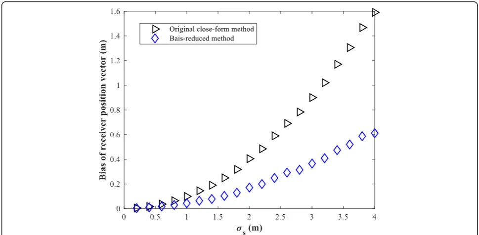
σRDOA= 2 m, and let σsvary from 0.2 to 4 m in

Fig. 5The RMSE of clock bias vector as measurement noise varies

intervals of 0.2 m. The simulation results are depicted in Figs. 9, 10, 11, 12, 13, and 14.

We draw the following conclusions from Figs. 9, 10,

11,12,13, and14.

1. The RMSEs of all estimates (including the source position, receiver position, and clock bias vector)

for both the proposed bias-reduced method and ori-ginal TSWLS algorithm can achieve the corre-sponding CRLBs at low noise levels, which verifies the theoretical derivation in Section5.

2. As the measurement noise or receiver position error increases, the original TSWLS algorithm gradually deviates from the CRLB after the

Fig. 7The bias of receiver position vector as measurement noise varies

thresholding effect occurs. However, the noise endurance threshold of the proposed method is always higher than that of the original TSWLS algorithm, which indicates that the proposed method is more robust to high noise levels than the original TSWLS algorithm.

3. The bias of the source position solution for both the proposed bias-reduced method and original

TSWLS algorithm coincides with the corresponding theoretical value under moderate noise levels, which validates the theoretical derivation in Sections 3 and 5.

4. Figures6,7,8,12, and14show that the proposed bias-reduced method can effectively reduce not only the bias of the source position but also the bias of the refined receiver positions and clock bias vector.

Fig. 9The RMSE of the source position as receiver position error varies

5. With an increase in measurement noise or receiver position error, the bias reduction of the proposed method is superior to that of the original TSWLS algorithm. Figure6shows that the bias of the source position estimated using the proposed method reduces by 288 m relative to the bias in the original TSWLS solution whenσs= 2 (m) andσRDOA= 6 (m).

6.2 Study of localization performance for different source ranges

According to the analysis in Remark 3, the proposed bias-reduced method is more effective for a far-field source. In this section, we examine the localization performance of the proposed method for different source ranges from the receivers. We fix the measurement noise level and receiver

Fig. 11The RMSE of clock bias vector as receiver position error varies

position error level asσRDOA= 2 m andσs= 2 m, respect-ively. Let source position u¼μuo_{, whereμrepresents the} distance factor that varies from 0.1 to 2. The other simula-tion condisimula-tions are the same as described in Subsecsimula-tion6.1. The simulation results for the RMSE and bias are shown in Figs.15,16,17,18,19, and20.

As expected, the improved bias of the proposed method is not obvious when the source is close to the receivers or even inside them (i.e., the distance factorμis small). How-ever, as the distance factor μincreases, the superiority of the proposed algorithm for bias reduction is gradually re-vealed. Moreover, the RMSE and bias of the source

Fig. 13The bias of receiver position vector as receiver position error varies

position solution for the proposed method coincide well with the corresponding CRLB and theoretical value, re-spectively, which again verifies the theoretical derivation in Section5.

6.3 Study of localization performance for different source positions

To highlight the superiority of the proposed

bias-reduced method, this subsection examines the

localization performance for 30 randomly placed sources. Assume that the source is randomly placed in a cubic region of 5 × 5 × 5 (km × km × km) around the point [15, 15, 15]T km. Fix the clock bias vector δ

= [40 60 80 100]T m and the receiver position

noise level σs= 2 m. Let σRDOA vary from 0.6 to 6 m

with 0.6 m intervals. The receiver positions and grouping situation are the same as described in

Sub-section 6.1. Figures 21, 22, and 23 show the boxplots

Fig. 15The RMSE of the source position as distance factor varies

[48] of the bias calculated using 30 random source

positions. For each source, we conduct L= 10000 MC

experiments.

These simulation results again validate that the proposed method has a smaller bias than the ori-ginal algorithm for all estimates including the source position, refined receiver positions, and clock bias

vector. Moreover, this improvement in reducing bias does not depend on the localization geometry.

7 Conclusions

This paper proposes a bias-reduced version for the well-known TSWLS solution using TDOAs in the pres-ence of receiver position errors and synchronization

Fig. 17The RMSE of clock bias vector as distance factor varies

clock bias. The new technique has two stages. In stage 1, through introducing an augmented matrix and imposing a quadratic constraint, the proposed method reduces the bias caused by the noise correlation of the WLS prob-lem. Stage 2 develops an effective WLS estimator to cor-rect the stage-1 solution, thereby avoiding the use of

nonlinear operations that increase the bias in the ori-ginal algorithm. Subsequently, the theoretical

perform-ance of the proposed method is derived via

second-order error analysis, demonstrating theoretically the effectiveness of the proposed method in reducing the bias and achieving the CRLB under moderate noise

Fig. 19The bias of receiver position vector as distance factor varies

for the far-field source. Finally, several simulation experi-ments are conducted to verify the superiority of the pro-posed method and the validity of the theoretical derivation. Several important conclusions can be drawn from the simulation results. (i) The RMSEs of all estimates (includ-ing the source position, receiver position, and clock bias vector) for the proposed method can achieve the corre-sponding CRLBs under moderate noise levels. (ii) The pro-posed method can reduce the bias of solution while not increasing the RMSE. (iii) The proposed method effectively reduces not only the bias of the source position but also the bias of the refined receiver positions and estimated

clock bias vector. (iv) As the source range increases, the bias reduction of the proposed method is more obvious. (v) The improvement of the proposed method in terms of reducing bias does not depend on the localization geometry.

Currently, the proposed method only uses TDOA in-formation of the emitted signal from a single target. Our future work will extend the proposed bias-reduced method to the following aspects:

1. Hybrid TDOA/FDOA localization

2. Localization in the multiple source scenario

(a)

(b)

Fig. 21The bias of source position for 30 randomly placed sources as measurement noise varies.aThe original algorithm.bThe proposed method

(a)

(b)

8 Appendix A

~

Applying the partitioned matrix inversion formula [49] and the definition ofBo₂in (29), we attain

Bo−1

Using (B.4), the definition ofG2in (13) and definition ofBo₃in below (40),Bo₃GT₂Bo₂−Tcan be reformulated as

Substituting (B.5) into (B.2) yields

EΔuΔuT¼ G~T₂B~−₂1 GoT₁ W1Go1

_~

B−21G~2

−1

¼EΔuΔuT ðB:6Þ

This completes the proof.

Abbreviations

3D:Three-dimensional; AOA: Angle of arrival; CRLB: Cramér–Rao lower bound; CTLS: Constrained total least-squares; FDOA: Frequency difference of arrival; GROA: Gain ratios of arrival; GSVD: Generalized singular value decomposition; MC: Monte Carlo; RDOA: Range difference of arrival; RMSE: Root mean square error; RSS: Received signal strength; TDOA: Time difference of arrival; TLS: Total least-squares; TOA: Time of arrival; TS: Taylor series; TSWLS: Two-step weighted least-squares; WLS: Weighted least-squares

Acknowledgements

The authors would like to thank the Editorial board and the Reviewers for considering and revising this manuscript. Meanwhile, we thank Glenn Pennycook, MSc, from Liwen Bianji, Edanz Group China (www.liwenbianji.cn/ac), for editing the English text of a draft of this manuscript.

Funding

This work is supported from the National Natural Science Foundation of China (Grant No. 61201381, No. 61401513 and No.61772548), China Postdoctoral Science Foundation (Grant No. 2016 M592989), the Self-Topic Foundation of Information Engineering University (Grant No. 2016600701), and the Outstanding Youth Foundation of Information Engineering University (Grant No. 2016603201).

Availability of data and materials

The datasets generated and/or analyzed during the current study are not publicly available but are available from the corresponding author on reasonable request.

Authors’contributions

XC and DW derived and developed the algorithm. XC and JY conceived of and designed the simulations. XC and YW performed the simulations. DW analyzed the results. XC wrote the manuscript. All authors read and approved the final manuscript.

Ethics approval and consent to participate

All data and procedures performed in paper were in accordance with the ethical standards of research community. This paper does not contain any studies with human participants or animals performed by any of the authors.

Consent for publication

Informed consent was obtained from all authors included in the study.

Competing interests

The authors declare that they have no competing interests.

Publisher’s Note

Springer Nature remains neutral with regard to jurisdictional claims in published maps and institutional affiliations.

Received: 17 July 2018 Accepted: 7 January 2019

References

1. A. Noroozi, M.A. Sebt, Target localization from bistatic range measurements in multi-transmitter multi-receiver passive radar[J]. IEEE Signal Processing Letters22(12), 2445–2449 (2015)

2. H. Ma, M. Antoniou, D. Pastina, F. Santi, F. Pieralice, M. Bucciarelli, M. Cherniakov, Maritime moving target indication using passive gnss-based bistatic radar[J]. IEEE Trans. Aerosp. Electron. Syst.54(1), 115_–130 (2018) 3. R. Amiri, F. Behnia, MAM Sadr, efficient positioning in momi radars with

widely separated antennas[J]. IEEE Commun. Lett.21(7), 1569–1572 (2017) 4. Y.L. Wang, Y. Wu, An efficient semidefinite relaxation algorithm for moving

source localization using TDOA and FDOA measurements[J]. IEEE Commun. Lett.21(1), 80–83 (2017)

5. C.W. Luo, L. Cheng, M.C. Chan, Y. Gu, J.Q. Li, Pallas: Self-bootstrapping fine-grained passive indoor localization using wifi monitors[J]. IEEE Trans. Mob. Comput.16(2), 466_–481 (2017)

6. T. Tirer, A.J. Weiss, Performance analysis of a high-resolution direct position determination method[J]. IEEE Trans. Signal Process.65(3), 544–554 (2017) 7. S. Tomic, M. Beko, R. Dinis, 3-D target localization in wireless sensor network

using RSS and AOA measurements[J]. IEEE Trans. Veh. Technol.66(4), 3197_– 3210 (2017)

8. C. Liu, D.Y. Fang, Z. Yang, H.B. Jiang, et al., RSS distribution-based passive localization and its application in sensor networks[J]. IEEE Trans. Wirel. Commun.15(4), 2883_–2895 (2016)

9. P.A. Forero, P.A. Baxley, L. Straatemeier, A multitask learning framework for broadband source-location mapping using passive sonar[J]. IEEE Trans. Signal Process.63(14), 3599–3614 (2015)

10. T. Chen, C.S. Liu, Y.V. Zakharov, Source localization using matched-phase matched-field processing with phase descent search[J]. IEEE J. Ocean. Eng.

37(2), 261–270 (2012)

11. Y.C. Hu, G. Leus, Robust differential received signal strength-based localization[J]. IEEE Trans. Signal Process.65(12), 3261_–3276 (2017) 12. R.M. Vaghefi, M.R. Gholami, R.M. Buehrer, E.G. Strom, Cooperative received

signal strength-based sensor localization with unknown transmit powers[J]. IEEE Trans. Signal Process.61(6), 1389–1403 (2013)

13. R. Niu, P.K. Varshney,Joint detection and localization in sensor networks based on local decisions[A], Proceedings of the Fortieth Asilomar Conference on Signals, Systems and Computers[C] (IEEE Press, Pacific Grove, 2006), pp. 525–529 14. D. Ciuonzo, P.S. Rossi, Distributed detection of a non-cooperative target

15. D. Ciuonzo, P.S. Rossi, P. Willett, Generalized rao test for decentralized detection of an uncooperative target[J]. IEEE Signal Processing Letters24(5), 678–682 (2017)

16. D. Ciuonzo, P.S. Rossi, Quantizer design for generalized locally-optimum detectors in wireless sensor networks[J]. IEEE Wireless Communications Letters7(2), 162–165 (2018)

17. K.C. Ho, M. Sun, Passive source localization using time differences of arrival and gain ratios of arrival[J]. IEEE Trans. Signal Process.56(2), 464_–477 (2008) 18. J.A. Luo, S.W. Pan, D.L. Peng, Z. Wang, Y.J. Li, Source localization in acoustic sensor networks via constrained least-squares optimization using AOA and GROA measurements[J]. Sensors18(4), 937 (2018)

19. W. Wang, G. Wang, J. Zhang, Y.M. Li, Robust weighted least squares method for TOA-based localization under mixed LOS/NLOS conditions[J]. IEEE Commun. Lett.21(10), 2226_–2229 (2017)

20. N. Wu, W.J. Yuan, H. Wang, J.M. Kuang, TOA-based passive localization of multiple targets with inaccurate receivers based on belief propagation on factor graph[J]. Digital Signal Processing49(C), 14_–23 (2016)

21. L. Yang, K.C. Ho, An approximately efficient TDOA localization algorithm in closed-form for locating multiple disjoint sources with erroneous sensor positions[J]. IEEE Trans. Signal Process.57(12), 4598_–4615 (2009) 22. K. Yang, J.P. An, X.Y. Bu, G.C. Sun, Constrained total least-squares location

algorithm using time-difference-of-arrival measurements[J]. IEEE Trans. Veh. Technol.59(3), 1558–1562 (2010)

23. K.H. Yang, G. Wang, Z.Q. Luo, Efficient convex relaxation methods for robust target localization by a sensor network using time differences of arrivals[J]. IEEE Trans. Signal Process.57(7), 2775–2784 (2009)

24. D. Wang, The geolocation performance analysis for the constrained Taylor-series iteration in the presence of satellite orbit perturbations[J]. Scientia Sinica Informations44(2), 231–253 (2014)

25. Z. Huang, L. J, Total least squares and equilibration algorithm for range difference location[J]. Electron. Lett.40(5), 121–122 (2004)

26. Y. Wang, K.C. Ho, TDOA positioning irrespective of source range[J]. IEEE Trans. Signal Process.65(6), 1447–1460 (2017)

27. G. Wang, A.M.C. So, Y.M. Li, Robust convex approximation methods for TDOA-based localization under NLOS conditions[J]. IEEE Trans. Signal Process.64(13), 3281–3296 (2016)

28. X.M. Qu, L.H. Xie, W.R. Tan, Iterative constrained weighted least squares source localization using TDOA and FDOA measurements[J]. IEEE Trans. Signal Process.65(15), 3990–4003 (2017)

29. K.C. Ho, X. Lu, L. Kovavisaruch, Source localization using TDOA and FDOA measurements in the presence of receiver location errors: analysis and solution[J]. IEEE Trans. Signal Process.55(2), 684–696 (2007) 30. Z. Wang, J.A. Luo, X.P. Zhang, A novel location-penalized maximum

likelihood estimator for bearing-only target localization[J]. IEEE Trans. Signal Process.60(12), 6166–6181 (2012)

31. S. Xu, K. Dogancay, Optimal sensor placement for 3D angle-of-arrival target localization[J]. IEEE Trans. Aerosp. Electron. Syst.53(3), 1196_–1211 (2017) 32. L. Kovavisaruch, K.C. Ho,Modified Taylor-series method for source and receiver

localization using TDOA measurements with erroneous receiver positions[A], Proceedings of the IEEE International Symposium on Circuits and Systems[C] (IEEE Press, Kobe, 2005), pp. 2295–2298

33. Y.T. Chan, K.C. Ho, A simple and efficient estimator for hyperbolic location[J]. IEEE Trans. Signal Process.42(4), 1905–1915 (1994)

34. L. X, K.C. Ho,Analysis of the degradation in source location accuracy in the presence of sensor location error[A], Proceedings of the IEEE International Conference on Acoustics, Speech and Signal Processing[C] (IEEE Press, Toulouse, 2006), pp. 14–19

35. Y. Wang, J. Huang, L. Yang, Y. Xue, TOA-based joint synchronization and source localization with random errors in sensor positions and sensor clock biases[J]. Ad Hoc Netw.27(C), 99–111 (2015)

36. Y. Wang, K.C. Ho, TDOA source localization in the presence of synchronization clock bias and sensor position errors[J]. IEEE Trans. Signal Process.61(18), 4532_–4544 (2013)

37. K. Dogancay, Bias compensation for the bearings-only pseudolinear target track estimator[J]. IEEE Trans. Signal Process.54(1), 59–68 (2006) 38. K.C. Ho, Bias reduction for an explicit solution of source localization using

TDOA[J]. IEEE Trans. Signal Process.60(5), 2101_–2114 (2012)

39. Y. Zhao, Z. Li, B.J. Hao, J.B. Si, P.W. Wan,Bias reduced method for TDOA and AOA localization in the presence of sensor errors[A], Proceedings of the IEEE International Conference on Communications[C] (IEEE Press, Paris, 2017), pp. 1_–6

40. Y. Liu, F.C. Guo, L. Yang, W.L. Jiang, An improved algebraic solution for TDOA localization with sensor position errors[J]. IEEE Commun. Lett.19(12), 2218–2221 (2015)

41. G. Wang, S. Cai, Y.M. Li, N. Ansari, A bias-reduced nonlinear WLS method for TDOA/FDOA-based source localization[J]. IEEE Trans. Veh. Technol.65(10), 8603_–8615 (2016)

42. B.J. Hao, L. Zan, P.H. Qi, L. GUAN, Effective bias reduction methods for passive source localization using TDOA and GROA[J]. SCIENCE CHINA Inf. Sci.56(7), 1–12 (2013)

43. R.J. Barton, D. Rao, Performance capabilities of long-range UWB-IR TDOA localization systems[J]. EURASIP Journal on Advances in Signal Processing

2008, 236791 (2007)

44. Y.T. Huang, J. Benesty, G.W. Elko, R.M. Mersereati, Real-time passive source localization: a practical linear-correction least-squares approach[J]. IEEE Transactions on Speech and Audio Processing9(8), 943–956 (2001) 45. Y.M. Ji, C.B. Yu, J.M. Wei, B. Anderson, Localization bias reduction in wireless

sensor networks[J]. IEEE Trans. Ind. Electron.62(5), 3004–3016 (2015) 46. T.K. Moon, W.C. Stirling,Mathematical methods and algorithms for signal

processing(Prentice-Hall, Upper Saddle River, NJ, 2000)

47. H.W. Sorenson,Parameter estimation: principles and problems(Marcel Dekker, New York, 1980)

48. M. Frigge, D.C. Hoaglin, B. Iglewicz, Some implementations of the boxplot[J]. Am. Stat.43(1), 50–54 (1989)