FULL PAPER
The Plasma Wave Experiment (PWE)
on board the Arase (ERG) satellite
Yoshiya Kasahara
1*, Yasumasa Kasaba
2, Hirotsugu Kojima
3, Satoshi Yagitani
1, Keigo Ishisaka
4,
Atsushi Kumamoto
2, Fuminori Tsuchiya
2, Mitsunori Ozaki
1, Shoya Matsuda
5, Tomohiko Imachi
1,
Yoshizumi Miyoshi
5, Mitsuru Hikishima
6, Yuto Katoh
2, Mamoru Ota
1, Masafumi Shoji
5, Ayako Matsuoka
6and Iku Shinohara
6Abstract
The Exploration of energization and Radiation in Geospace (ERG) project aims to study acceleration and loss mecha-nisms of relativistic electrons around the Earth. The Arase (ERG) satellite was launched on December 20, 2016, to explore in the heart of the Earth’s radiation belt. In the present paper, we introduce the specifications of the Plasma Wave Experiment (PWE) on board the Arase satellite. In the inner magnetosphere, plasma waves, such as the whistler-mode chorus, electromagnetic ion cyclotron wave, and magnetosonic wave, are expected to interact with particles over a wide energy range and contribute to high-energy particle loss and/or acceleration processes. Thermal plasma density is another key parameter because it controls the dispersion relation of plasma waves, which affects wave–par-ticle interaction conditions and wave propagation characteristics. The DC electric field also plays an important role in controlling the global dynamics of the inner magnetosphere. The PWE, which consists of an orthogonal electric field sensor (WPT; wire probe antenna), a triaxial magnetic sensor (MSC; magnetic search coil), and receivers named electric field detector (EFD), waveform capture and onboard frequency analyzer (WFC/OFA), and high-frequency analyzer (HFA), was developed to measure the DC electric field and plasma waves in the inner magnetosphere. Using these sensors and receivers, the PWE covers a wide frequency range from DC to 10 MHz for electric fields and from a few Hz to 100 kHz for magnetic fields. We produce continuous ELF/VLF/HF range wave spectra and ELF range waveforms for 24 h each day. We also produce spectral matrices as continuous data for wave direction finding. In addition, we inter-mittently produce two types of waveform burst data, “chorus burst” and “EMIC burst.” We also input raw waveform data into the software-type wave–particle interaction analyzer (S-WPIA), which derives direct correlation between waves and particles. Finally, we introduce our PWE observation strategy and provide some initial results.
Keywords: Plasma wave, Radiation belt, Geospace, Inner magnetosphere, Chorus
© The Author(s) 2018. This article is distributed under the terms of the Creative Commons Attribution 4.0 International License (http://creativecommons.org/licenses/by/4.0/), which permits unrestricted use, distribution, and reproduction in any medium, provided you give appropriate credit to the original author(s) and the source, provide a link to the Creative Commons license, and indicate if changes were made.
Open Access
*Correspondence: kasahara@is.t.kanazawa-u.ac.jp
1 Graduate School of Natural Science and Technology, Kanazawa University, Kakuma, Kanazawa 920-1192, Japan
Full list of author information is available at the end of the article Introduction
In the Earth’s magnetosphere, various plasma phenomena simultaneously occur at various time, spatial, and energy scales. The generation and disappearance mechanisms of the Earth’s radiation belt are critical issues in space weather and the science of magnetized planets, such as Jupiter and Saturn. It is well known that the high-energy particle population trapped in the Earth’s radiation belt
significantly changes during the magnetically disturbed period of magnetic storms and high-speed solar wind streams (HSS) (e.g., Paulikas and Blake 1979; Reeves et al.
from the VLF instruments (Kimura et al. 1990) on board the Akebono satellite. This study clarified that the whis-tler-mode chorus is primarily located near the inner edge of the outer radiation belt (L ~ 2.5) and gradually shifts outward (L ~ 4) with time and that the total wave energy generated during the storm is large enough to accelerate relativistic electrons. Recently, Miyoshi et al. (2013) dem-onstrated that whistler-mode waves accelerate relativistic electrons during HSS events with southward interplan-etary magnetic field (IMF)-dominant HSS (SBz-HSS), while this acceleration mechanism is not effective during HSS events with northward IMF-dominant HSS (NBz-HSS). They finally suggested that the responses of the outer radiation belt flux depend on the whistler-mode wave-electron interactions that are associated with a series of sub-storms.
It is well established that there are various types of plasma waves other than the whistler-mode chorus in the equatorial region, such as electromagnetic ion cyclotron wave (EMIC) (Young et al. 1981; Kasahara et al. 1992; Sakaguchi et al. 2013; Min et al. 2012; Usanova et al.
2012; Matsuda et al. 2014a; and the references therein) and magnetosonic wave (MSW) (Laakso et al. 1990; Kasahara et al. 1994; Fraser and Nguyen 2001; Santo-lik et al. 2004, 2016; and the references therein). It was also suggested that in addition to the whistler-mode cho-rus, the MSW plays an important role in acceleration processes in the inner magnetosphere (e.g., Horne et al.
2007; Meredith et al. 2008). On the other hand, pitch angle scattering caused by the EMIC is thought to be one plausible loss mechanism that contributes to relativistic electron precipitation (Miyoshi et al. 2008; Jordanova et al. 2008; Shprits et al. 2016). Furthermore, there are additional suggestions that plasmaspheric hiss (Brene-man et al. 2015) and VLF radio transmitters (Baker et al.
2014) could play important roles in the electron loss pro-cess in the radiation belt.
As described above, plasma waves from several Hz to a few tens of kHz, such as the whistler-mode chorus, EMIC, and MSW, are expected to interact with charged particles over a wide energy range from a few eV to MeV and contribute to high-energy particle loss and/or accel-eration processes in the inner magnetosphere. In these processes, thermal plasma density is a key parameter because it controls plasma wave dispersion relations, which affect wave–particle interaction conditions and wave propagation characteristics. In addition, DC electric field also plays an important role in controlling the global dynamics of the inner magnetosphere (e.g., Nishimura et al. 2007; Thaller et al. 2015; and the references therein).
Computer simulation is a powerful tool that can be used to understand the complex physical processes in the inner magnetosphere. Recent computer simulations have
clarified that the chorus emission is effectively generated in the region close to the magnetic equator through non-linear wave–particle interactions (e.g., Katoh and Omura
2007; Omura et al. 2008). Omura (2014) reviewed a non-linear theory of the generation mechanism of chorus emission, describing the nonlinear dynamics of resonant electrons and the electromagnetic electron “hole” for-mation in phase space that results in resonant currents generating rising-tone emissions. Conversely, falling-tone emissions are generated through the formation of electron “hills” (Omura 2014). Katoh and Omura (2016) carried out a self-consistent simulation of the whistler-mode chorus generation process and showed that simu-lated spectral fine structures were similar to the Cluster spacecraft observation. They also suggested that oblique propagation of waves with respect to the magnetic field is essential for forming the half gyrofrequency gap. Omura et al. (2015) demonstrated that chorus emissions can accelerate electrons from tens of keV to several MeV within a few minutes and that nonlinear trapping pro-cesses [i.e., relativistic turning acceleration (RTA) and ultra-relativistic acceleration (URA)] form a dumbbell distribution of relativistic electrons.
Wave–particle interactions related to EMIC waves have also been vigorously studied. Shoji and Omura (2014) performed parametric analyses of EMIC-triggered emis-sions with a gradient of non-uniform ambient magnetic field using a hybrid simulation. Nakamura et al. (2015) investigated sub-packet structures found in EMIC rising-tone emissions observed by THEMIS, showing that the time evolution of the observed frequency and amplitude can be reproduced consistently by nonlinear growth theory. Kubota et al. (2015) performed test particle sim-ulations of relativistic electrons interacting with EMIC-triggered emissions in the plasmasphere and concluded that EMIC-triggered emissions can efficiently precipitate electrons at 0.5–6 MeV.
The Exploration of energization and Radiation in Geo-space (ERG) project aims to study relativistic electron acceleration and loss mechanisms around the Earth (Miyoshi et al. 2012, 2017). The ERG satellite, launched on December 20, 2016, and nicknamed “Arase,” is a satel-lite to explore the Earth’s radiation belt using electric and magnetic field instruments and electron and ion detec-tors covering wide frequency and energy ranges, respec-tively. The inclination of the Arase is 31°, and the altitudes of the apogee and perigee are ~ 32,000 and 460 km, respectively. The orbital period is approximately 570 min. The Arase satellite is a spin-stabilized satellite, with its spin axis pointed 15° toward the sun (within 4°–20°) and a spin period of ~ 8 s.
et al. 2012, 2017). Conjugate observations of the Arase and the ground observation network are important in comprehensive understanding of particle precipita-tion processes, as consequences of wave–particle inter-actions. Furthermore, collaborative studies between observation and simulation are essential to clarify the multiscale plasma dynamics, in which macroscopic and microscopic processes complicatedly occur interacting with each other, in the inner magnetosphere. In these contexts, measurements of plasma waves are required to cover wide frequency ranges in both electric and mag-netic fields to observe various plasma waves interacting with ions and electrons over wide energy ranges. In par-ticular, it is very important to capture continuous wave-form as long as possible with a precise time resolution to analyze the phase difference between wave packets and particles, and also the time difference between measure-ments by the Arase and ground-network stations.
The NASA Van Allen Probes, formerly called Radia-tion Belt Storm Probes (RBSP), began their observaRadia-tions of the inner magnetosphere in 2012 (Mauk et al. 2013), prior to the launch of the Arase satellite. As for the meas-urements of the DC electric field and plasma waves, the EFW (Wygant et al. 2013) and the EMFISIS (Kletzing et al. 2013) on board the Van Allen Probes have resulted in many scientific achievements over the past 5 years. Although the orbit of the Arase satellite is quite similar to the orbits of the Van Allen Probes, the inclination of Arase (31°) is much larger than the ones of Van Allen Probes (~ 10°), which will allow for the ability to explore not only the equatorial region but also the off-equatorial region. We expect to measure plasma waves such as cho-rus and EMIC propagating from their generation regions near the equatorial plane and derive their plasma wave properties (e.g., wave normal direction and Poynting flux) that could be also important key parameters to clar-ify the wave–particle interaction along their propagation paths in the off-equatorial region.
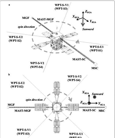
Figure 1 shows an overview of the Arase satellite. The “SGA” subscript in the coordinate system stands for “Spinning Satellite Geometry Axis” coordinates, which represent the geometrical positions of the components on board the satellite. The Arase has two sets of MAST named MAST-MGF and MAST-SC. A triaxial fluxgate magnetometer (referred to as MGF) is mounted on the top of the MAST-MGF to measure magnetic fields from DC to a few tens of Hz (Matsuoka et al. 2018). On the top of the MAST-SC, a triaxial magnetic search coil (referred to as MSC) is mounted to measure AC mag-netic fields from a few Hz to 100 kHz (Ozaki et al. 2018). The WPT consists of four wire antennas (wire probe antenna sensor; WPT-S) to measure electric fields from DC to 10 MHz (Kasaba et al. 2017). The branch numbers
attached after S (i.e., S1, S2, WPT-S3, and WPT-S4) are the serial numbers of the WPT-S component, and we hereafter call them as WPT-S-U1 and WPT-S-U2 oriented in the u-axis and WPT-S-V1 and WPT-S-V2 oriented in the v-axis, with respect to the observation axis. Details of the relationship among coordinates defined for the MSC and WPT-S is provided in “Overview” section. The lengths of each MAST and WPT-S are 5 and 15 m, respectively, which are deployed in the satellite spin plane.
Nine scientific instruments are installed in the Arase satellite to comprehensively measure charged parti-cles, DC electric and magnetic fields, and plasma waves (Miyoshi et al. 2012, 2017). The most distinctive part of the Arase satellite is the installation of the software-type wave–particle interaction analyzer (S-WPIA) (Katoh et al. 2018; Hikishima et al. 2018). The S-WPIA is a soft-ware module that functions as a “WPIA,” an innovative instrument that was originally proposed by Fukuhara et al. (2009). The WPIA measures wave–particle interac-tions directly and quantitatively by calculating the cor-relations between particles and waveforms (Katoh et al.
2013; Kitahara and Katoh 2016). To realize the S-WPIA, a huge data storage named mission data recorder (MDR) with a capacity of 32 GB was installed on board the Arase. The S-WPIA stores raw data measured by the onboard instruments in the MDR to perform correlation analyses between particles and waveforms.
The Plasma Wave Experiment (PWE) is one of instru-ments on board the Arase satellite to measure plasma waves and DC electric field. The PWE was elaborately designed to obtain maximum scientific outputs in coop-eration with the S-WPIA and other scientific instru-ments. In the present paper, we introduce the PWE specifications and initial results following the launch of Arase. In the following section, we introduce the PWE specifications. Next, we describe the electromagnetic compatibility (EMC) requirements applied to the Arase satellite to guarantee the quality of plasma wave meas-urements. In the following two sections, we introduce our observation strategy of the PWE and provide some initial results obtained by the PWE, respectively. Finally, we summarize the present study and our findings.
PWE instrumentation Overview
X
SGAY
SGAZ
SGAWPT-S-U1
(WPT-S1)
WPT-S-V1
(WPT-S3)
WPT-S-V2
(WPT-S4)
Sunward
spin direction
WPT-S-U2
(WPT-S2)
X
SGAY
SGAZ
SGASunward
spin direction
WPT-S-V1
(WPT-S3)
WPT-S-U1
(WPT-S1)
WPT-S-V2
(WPT-S4)
a
b
MAST-SC
MAST-MGF
MSC
MGF
MAST-MGF
MAST-SC MSC
MGF
WPT-S-U2
(WPT-S2)
X
SGAY
SGAZ
SGAWPT-S-U1
(WPT-S1)
WPT-S-V1
(WPT-S3)
WPT-S-V2
(WPT-S4)
Sunward
spin direction
WPT-S-U2
(WPT-S2)
X
SGAY
SGAZ
SGASunward
spin direction
WPT-S-V1
(WPT-S3)
WPT-S-U1
(WPT-S1)
WPT-S-V2
(WPT-S4)
a
b
MAST-SC
MAST-MGF
MSC
MGF
MAST-MGF
MAST-SC MSC
MGF
WPT-S-U2
(WPT-S2)
and onboard frequency analyzer (WFC/OFA), and high-frequency analyzer (HFA).
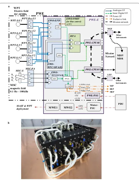
Figure 2a shows the block diagram of the PWE system. The WPT consists of two sets of orthogonal wire anten-nas dedicated to measuring the electric field. The MSC is the magnetic field sensor mounted on the top plate of the MAST with a length of 5 m to avoid electromagnetic contamination radiated from the satellite. The PWE-E is the main electronics box and is shown in Fig. 2b. The followings are the main components contained in the PWE-E.
The EWO (EFD/WFC/OFA) is an abbreviation, gener-ated from the initials of the EFD, WFC, and OFA receiv-ers. The EWO-EFD and EWO-WFC/OFA(E) are the receiver components responsible for electric field meas-urements, and the signals detected by the WPT sen-sor (WPT-S) are fed into these components through the preamplifiers (WPT-Pre). The EWO-EFD is dedicated to measuring the DC and very low-frequency electric fields, while the EWO-WFC/OFA(E) is the electric field receiver measuring from 10 Hz to 100 kHz. The EWO-WFC/ OFA(B) is the magnetic field receiver and the signals from the MSC sensors (MSC-S) are fed into the EWO-WFC/OFA(B) through the preamplifiers (MSC-PA). The HFA is the high-frequency electric and magnetic field receiver, into which two electric field components from the WPT-S and one magnetic field component from the MSC-S are fed (Kumamoto et al. 2018). Clock signals called “S-WPIA clock” are distributed from the PWE to the S-WPIA cooperative particle detectors named XEP (Extremely High-Energy Electron Experiments), HEP (High-Energy Electron Experiments) and MEP (Medium-Energy Particle Experiments) (Miyoshi et al. 2017) through three dedicated lines. As the S-WPIA observa-tion requires both high time resoluobserva-tion and high rela-tive time precision among the instruments, the S-WPIA clock is used to guarantee that the relative observation time precision is much better than 10 μs between the particle detectors and the PWE.
Two independent CPU boards (CPU#8 and CPU#9) are installed in the PWE-E. The design of the CPU board is common among the onboard scientific instruments, and ‘#8’ and ‘#9’ represent the serial numbers of the CPU boards for the scientific instruments on board the Arase. The CPU#8 is responsible for processing signals from the electric field receivers, and the digital data from the EWO-EFD, EWO-WFC/OFA(E) and HFA are fed into the CPU#8. The CPU#9 is responsible for processing sig-nals for the magnetic components that are digitized by the EWO-WFC/OFA(B). The CPU boards are mutually connected to form a mission network in the spacecraft. The CPU#8 and #9 assigned for the PWE are connected with the MGF (Matsuoka et al. 2018) and the Low-Energy
Particle Experiments (LEP) (Kazama et al. 2017; Asamura et al. 2018), respectively, as shown in Fig. 2a. The mission data processed by these CPU boards are transferred to the mission data processor (MDP), shown on the right in Fig. 2a, through the mission network in the spacecraft (Takashima et al. 2018).
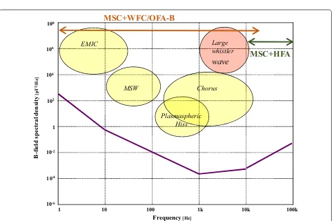
The MWE (MAST/WPT-S Electronics) is the electron-ics for extension control of the MAST and WPT-S. (The MWE1 is responsible for the extension control of the WPT-S-U1, WPT-S-U2, and the MAST. The MWE2 is responsible for the extension control of the WPT-S-V1 and WPT-S-V2.) The power supply units (PSU) for the instruments as well as extension motors and power dis-tributor (IPD; Instruments power disdis-tributor) are also implemented in the PWE-E. The mass and power con-sumption of the PWE is summarized in Tables 1 and 2.
Figure 3 shows the PWE sensor configurations and the coordinate systems. In this figure, the spinning sat-ellite geometry axis (SGA) coordinates are represented by X, Y, Z. In the SGA coordinates, the spin axis of the satellite is defined as the ZSGA-axis, and the MAST-SC
is directed toward the positive Y-direction. The WPT is radially deployed and directed in the ±u and ±v direc-tions. Coordinates u and v are orthogonal and deviate by 133.5° anticlockwise from the +XSGA and +YSGA
direc-tions, respectively. On the other hand, the coordinate systems for the MSC are defined by the symbols (α, β, γ), where α and β deviate by 45° clockwise from the +XSGA
and +YSGA directions, respectively, and γ is parallel to
the + ZSGA direction.
The main scientific objectives of the PWE are as follows:
1. To obtain measurements of waveforms and spectra of whistler-mode chorus, MSW, EMIC, etc., and to clarify the mechanisms of acceleration/loss of radia-tion belt particles through interacradia-tion with plasma waves, as well as the generation and propagation characteristics of plasma waves in the inner magne-tosphere.
2. To obtain measurements of the DC electric field, which is thought to play an important role in the development of plasma outflow from the plasmas-phere during magnetic storms, plume formation, and enhancement of injection processes of ring current particles. It is also important to clarify the genera-tion mechanism of the global DC electric field and its growth process.
tem-Bα
Bβ
Bγ
WPT-S-U1 EWO-EFD
EWO-WFC/OFA(E)
EWO-WFC/OFA(B)
PWE-CPU#8
MSC-PA
PWE-E
MDP/ MDR HFA
MGF
PDU ADC
ADC
EWO-99MV (for Bias control)
99V
MSC-S
WPT-Pre-U1
Mission Network
PWE-PSU 12V
+5V +3.3V
PWE
MWE1 MWE2 Motor-PSU
ADC FPGA
WPT
Electric field DC-10MHz
MSC
magnetic field 0.1 Hz – 100kHz WPT-S-U2WPT-Pre-U2
WPT-S-V1WPT-Pre-V1
WPT-S-V2WPT-Pre-V2
ADC
+28V +15V
PWE-CPU#9
LEP
MAST & WPT deployment
Other instruments Other instruments
Analogue I/F Inner Digital I/F Power I/F
Mission network
LVDS XEP
HEP MEP
Exclusive link
S-WPIA clock S-WPIA clock S-WPIA clock a
b
perature profile in the inner magnetosphere during magnetic storms. Another aim is to understand the generation and mode conversion processes of elec-tromagnetic waves.
In addition to the objectives mentioned above, we expect to estimate ion constituents of background plasma derived from characteristic frequencies of EMIC waves in multiple component plasma. As EMIC waves exhibit characteristic frequencies, such as lower hybrid resonance and cutoff frequencies (Matsuda et al. 2014a,
b, 2015, 2016), it is possible to estimate constituents of cold ions from these characteristic wave frequencies.
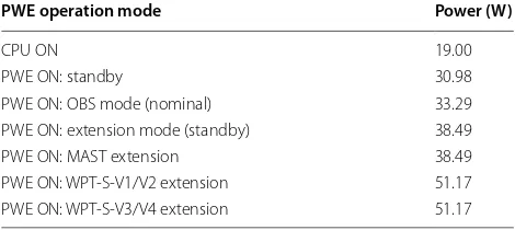
Finally, we show characteristic frequencies and inten-sities of expected wave phenomena in Fig. 4. The sen-sitivities and frequency coverage of the electric field measurements using the WPT and the receivers (EFD, WFC/OFA(E), and HFA) are also shown. Figure 5
shows the characteristic frequencies and intensities of
Table 1 PWE component masses
PWE (total) 14.549 kg
PWE-E 6.335 kg
WPT-PRE 0.733 kg (for four units)
WPT-S 3.059 kg (for four units)
MSC-PA 0.688 kg
MAST-MSC (including the MSC-S) 3.734 kg
Table 2 PWE power consumption
PWE operation mode Power (W)
CPU ON 19.00
PWE ON: standby 30.98
PWE ON: OBS mode (nominal) 33.29 PWE ON: extension mode (standby) 38.49
PWE ON: MAST extension 38.49
PWE ON: WPT-S-V1/V2 extension 51.17 PWE ON: WPT-S-V3/V4 extension 51.17
1 10 100 1k 10k 100k 1M 10M
10-6
10-8
10-10
10-12
10-4
10-2
1
102
104
Frequency[Hz]
E-field
spectral densit
y
[mV
2/m 2/Hz]
Chorus
Plasmaspheric Hiss EMIC
AKR (potential)
WPT-Pre(AC) + WFC/OFA-E WPT-Pre(DC) + EFD
WPT-Pre(AC) + HFA
MSW
ECH
Continuum UHR
Fig. 4 Electric field wave phenomena as the scientific targets of the ERG mission, and electric field sensor sensitivities and frequency coverage using the WPT and the receivers (EFD, WFC/OFA(E), and HFA)
1 10 100 1k 10k 100k
Plasmaspheric Hiss
MSC+WFC/OFA-B
Chorus Large whistler
wave
MSC+HFA
EMIC
B-field
spectral
densit
y
[p
T
2/Hz
]
Frequency[Hz]
10-6
10-4
10-2
1
102
104
106
108
MSW
expected wave phenomena as well as the sensitivities and frequency coverage of the magnetic field measure-ments using the MSC and the receivers (WFC/OFA(B), and HFA). As shown in these figures, the sensitivity and frequency coverage of the PWE allow it to measure all expected plasma waves and radio waves in the inner mag-netosphere. In the following subsections, we describe the subcomponents of the PWE.
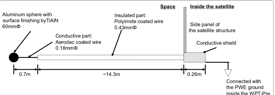
WPT
The WPT is designed to pick up the electric field from DC to 10 MHz. As shown in Fig. 6, the total length of the WPT is 15 m (32 m from tip to tip), and a 60-mm-diameter sphere is attached to the end of a sensor wire. Apart from the upper 70 cm, the wire is covered by poly-imide insulator. These wires extend orthogonally in the spacecraft spin plane, almost perpendicular to the Sun. This system is similar to the WPT that was developed for the Plasma Wave Investigation (PWI) (Kasaba et al. 2010) on board the BepiColombo Mercury Magnetospheric Orbiter (MMO), except that aluminum alloy was used to reduce the sphere probe mass (as opposed to titanium alloy in the MMO). The detailed specifications and per-formance of the WPT developed for the Arase are pre-sented in Kasaba et al. (2017).
MSC
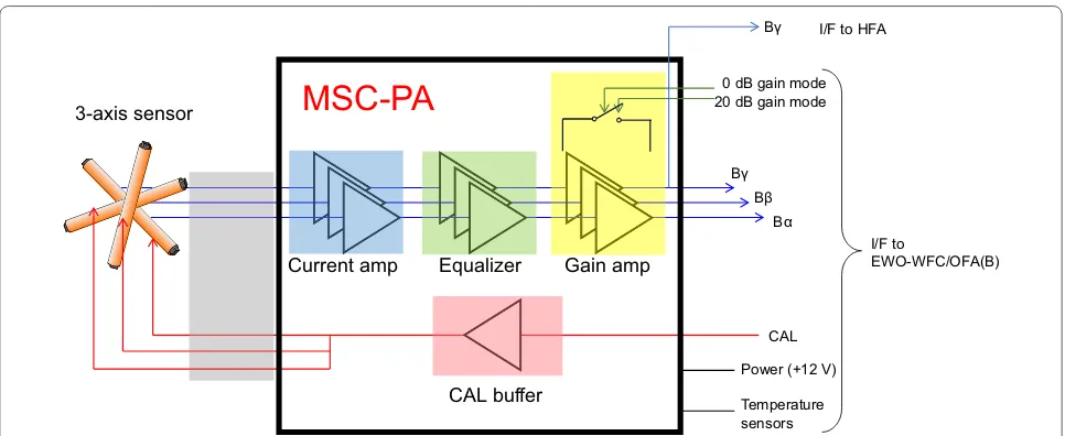
The AC magnetic field vector observations are essential for probing plasma waves. The magnetic field observa-tions are generally performed using search coil mag-netometers for low-frequency bands (less than several tens of kHz) and loop antennas for high-frequency bands (over 100 kHz). The Arase satellite carries a triaxial search coil magnetometer to measure the whistler-mode waves
below the local electron cyclotron frequency, which is the main target of the mission. The MSC is inherited from the AKEBONO (Fukunishi et al. 1990), GEOTAIL (Mat-sumoto et al. 1994), and MMO (Kasaba et al. 2010) mis-sions. The MSC on board the Arase was developed based on the design for the future MMO spacecraft because the flight model for the MMO was constructed in advance for the Arase. Figure 7 shows the block diagram of the MSC. The MSC adopts a current-sensitive amplifier (Ozaki et al. 2014) instead of a common voltage amplifier using the flux feedback technique (Matsumoto et al. 1994). The advantages of the current-sensitive amplifier include a lower input impedance and an elimination of the flux feedback coil. The disadvantage is that it consumes more power than the voltage amplifier using the flux feedback, as an equalizer is required to improve the signal dynamic range. This problem was, however, solved by low power applications using application-specific integrated circuits (ASIC) technology (Ozaki et al. 2014, 2016).
Three components of the magnetic field below 20 kHz detected by the MSC are fed to the WFC/OFA(B), and one component of the magnetic field along the satellite spin axis from 10 to 100 kHz is fed to the HFA. Each sen-sor of the MSC has a gain adjustment amplifier to avoid signal saturation by abnormally large-amplitude whistler-mode waves in the radiation belts (Cattell et al. 2008). The saturation levels for high and low gains are 1 and 10 nT, respectively, at 1 kHz. The EWO-WFC/OFA(B) supplies the gain control signal, squared pulses for cali-bration, and power line. The MSC covers a frequency range from a few Hz to 100 kHz. The noise equivalent magnetic induction is 20 fT/Hz1/2 (femto-Tesla/Hz1/2) at
1 kHz, and the nominal power consumption is 0.43 W
Aluminum sphere with
with a 12-V supply. A detailed description of the MSC performance is available in Ozaki et al. (2018).
EFD
The EFD measures DC and extremely low-frequency electric field. Two types of measurements, single probe (SPB) and double probe (DPB), are performed by the EFD. As shown in Fig. 3, the SPB provides four channels of satellite potential (i.e., Vu1, Vu2, Vv1, and Vv2) using the
four sets of WPT-S independently at a sampling rate of 128 Hz. The dynamic range of the SPB is ± 100 V. The satellite potential is an important diagnostic of elec-tron density in combination with the UHR frequency, measured by the HFA. The DPB provides two channels of differential signals (Eu and Ev shown in Fig. 3) that
are measured by the two pairs of orthogonal WPT at a 512 Hz sampling rate. The dynamic range of the DPB is nominally ± 200 mV/m, but data with a dynamic range of
± 3 V/m and a sampling rate of 128 Hz can be also pro-vided from the SPB output using onboard software. The DPB is dedicated to measuring the DC electric field and ion mode waves, such as EMIC. The waveforms measured by the DPB are expected to be analyzed by combining the magnetic waveforms measured by the MGF (Matsuoka et al. 2018). Detailed specifications and performance of the EFD are presented in Kasaba et al. (2017).
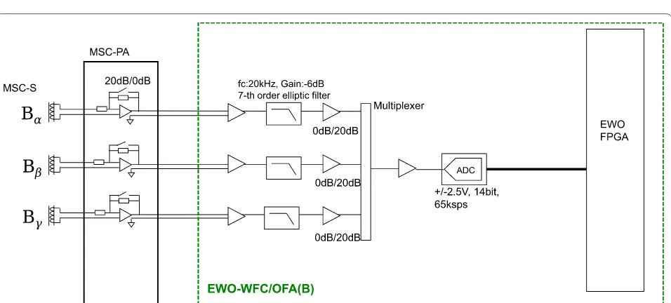
Waveform capture/onboard frequency analyzer
The WFC and OFA are dedicated to measuring plasma waves between 10 Hz and 100 kHz for the two electric field components and between 10 Hz and 20 kHz for the three magnetic field components. The alternative upper
frequency bound of 20 and 120 kHz for the electric field components is selected by the telemetry command. The WFC/OFA covers the crucial frequency range, in which chorus waves, hiss waves, and magnetosonic waves appear. The WFC and OFA share the same analog cir-cuits. While the WFC provides the time domain data as waveforms, the OFA outputs digitally processed fre-quency domain data from the waveforms. Figures 8 and
9 show the block diagrams of the WFC/OFA(E) and WFC/OFA(B), respectively, as well as their sensors and preamplifiers.
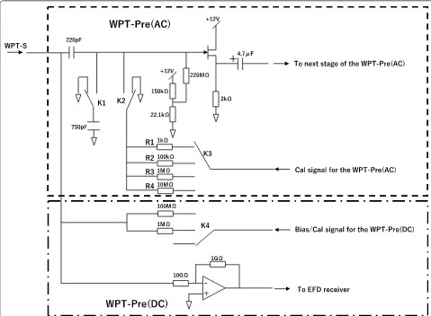
Preamplifier for the plasma wave electric field component
The electric fields picked up by the WPT-S are fed into the WFC/OFA(E) through its preamplifier (WPT-Pre). The PWE has two types of preamplifiers, depending on their frequency range coverage (Kasaba et al. 2017). Figure 10 shows the simplified front-end circuit of the preamplifiers for the electric field measurements. The WPT-Pre (DC) covers the signal at lower frequencies from DC to ~ 200 Hz, while the WPT-Pre (AC) is dedi-cated to measuring frequencies above a few Hz. Details of the WPT-Pre (DC) are described by Kasaba et al. (2017). The output of the WPT-Pre (AC) is connected to the WFC/OFA(E) input, which is also shared by the HFA (Kumamoto et al. 2018).
The antenna impedance of the electric field sensor strongly depends on plasma parameters, such as plasma density and temperature, which implies that the imped-ance varies by satellite location. Since the efficiency of electric field antenna detection is related to its antenna impedance, the input impedance of the preamplifier
CAL buffer
Current amp Equalizer Gain amp
MSC-PA
0 dB gain mode20 dB gain mode
Bγ Bβ
Bα Bγ
CAL
Power (+12 V)
Temperature sensors
I/F to
EWO-WFC/OFA(B) I/F to HFA
3-axis sensor
should be much higher than the expected antenna impedance to pick up electric field component of plasma waves regardless of satellite location. In WPT-Pre (AC) design the input impedance is 220 MΩ. As we adopt a
decoupling capacitance of 220 pF, a high-pass filter (HPF) with a cutoff frequency of 3 Hz is formed. The filter eliminates ultra-low-frequency waves as well as the elec-tric field caused by V×B, through the spacecraft spin
0dB / -20dB
fc:120kHz, Gain:-6dB 7-th order elliptic filter
fc:20kHz, Gain:-6dB 7-th order elliptic filter
Level shifter Gain: +4dB
+/-2.5V, 14bit 256ksps(Intermittent) 65ksps(Continuous)
ADC EX+
CAL
EX-CAL
50Ω
50Ω
HFA(EX-) WPT-Pre-U1
HFA(EX+)
ADC WPT-Pre-U2
0dB/20dB/40dB/60dB WPT-S-U1
WPT-S-U2
0dB / -20dB
CAL
CAL
WPT-Pre-V1
WPT-Pre-V2 WPT-S-V1
WPT-S-V2
HFA(EY-)
HFA(EY+) 50Ω
EWO-WFC/OFA(E) 50Ω
Main amplifier
fc:120kHz, Gain:-6dB 7-th order elliptic filter
fc:20kHz, Gain:-6dB 7-th order elliptic filter
+/-2.5V, 14bit 256ksps(Intermittent) 65ksps(Continuous)
Level shifter Gain: +4dB
Main amplifier
0dB/20dB/40dB/60dB
*Switch
*1
*2
*3
*4 *a
*b
*c
*d
*a *b *c *d
Nominal *1 *2 *3 *4
Monopole *3 GND *4 GND
*switch combination
Fig. 8 Simplified block diagram of the WPT and EWO-WFC/OFA(E). Two sets of differential signals between WPT-S-U1 and WPT-S-U2, and WPT-S-V1 and WPT-S-V2 are fed to the WFC/OFA(E) in the “Nominal mode”, while the WPT-S-V1 and WPT-S-V2 are connected to each electric field channel of the WFC/OFA(E) and both are used as monopole antennas in the “Monopole mode”
motion, typically at a frequency of 1/8 Hz. Here, V and
B denote the satellite velocity and the ambient magnetic
field, respectively.
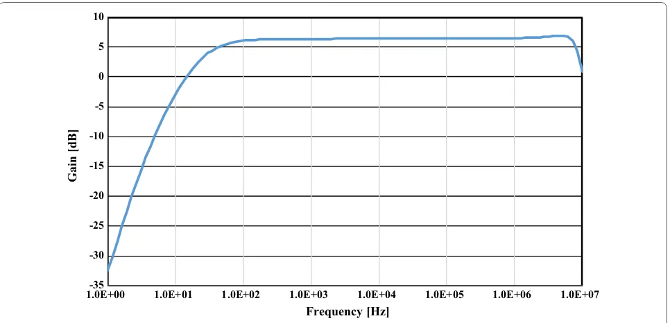
The WPT-Pre (AC) has an alternative gain control that is selected by the telemetry command. Figure 11 shows the frequency response of the WPT-Pre (AC) in high gain mode. As shown in the upper panel, the WPT-Pre (AC) covers frequencies above a few 10 Hz at approxi-mately 6 dB gain. As the loss at the WPT-S input exists in the coupling with its input capacitance, peripheral capacitance, and the antenna impedance, the total gain of the WPT-Pre (AC) accounting for antenna impedance is almost unity. “Onboard calibration system” section describes the equivalent circuit, which considers the cou-pling of the WPT-Pre (AC) input and the WPT-S.
The attenuation at the WPT-Pre (AC) input is effective by turning on the K1 switch (Fig. 10) in low-gain mode. The 750-pF capacitance attenuates the detected plasma waves in combination with the antenna impedance. This means that the precise attenuation level primarily
depends on the ratio of the antenna impedance to the 750-pF capacitance. Using the onboard calibration sys-tem, described in “Onboard calibration system” sec-tion, the precise preamplifier gain in low-gain mode is measured.
The precise electric field sensitivity, displayed in Fig. 4, can be obtained from the flight data of the WPT-Pre (AC) after launch. The sensitivity shown in Fig. 4 is obtained by assuming 70 pF, 10 MΩ and 15 m for the theoretical antenna capacitance in vacuum, typical plasma imped-ance, and the effective length of the WPT-S, respectively.
The identification of the electric field antenna imped-ance is necessary to calibrate the observed electric field data. In particular, since waveform data contain the phase information, the precise phase calibration (considering the antenna impedance) using the PWE onboard calibra-tion system is very important. The system inputs known waveforms at the WPT-Pre (AC) input through different resistances (R1, R2, R3, and R4 shown in Fig. 10). The
detailed function of the onboard calibration system is described in “Onboard calibration system” section.
Main receivers
As shown in Figs. 8 and 9, each channel of the WFC/ OFA consists of a differential amplifier, a low-pass filter (LPF) as the antialiasing filter, a main amplifier, an A/D converter, and a digital processing part. The LPF is the seventh-order elliptic filter that avoids the aliasing effect at the A/D converter.
For the electric field channels (Fig. 8), two sets of the LPF with different cutoff frequencies are installed. These cutoff frequencies are 20 and 120 kHz, and can be selected by the telemetry command. In the nominal operation, 20 kHz is used for the cutoff LPF value. For the magnetic field channel, one LPF with a 20-kHz cutoff fre-quency is used.
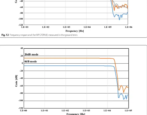
The gains of the main amplifier can be controlled in four steps for electric field channels and in two steps for magnetic field channels. Figures 12 and 13 show the frequency responses of the WFC/OFA for electric and magnetic field channels, respectively. As shown in these figures, the gain of the electric field channels varies from 0 to 60 dB, while the magnetic field channel gains vary from 0 to 20 dB by 20 dB step. The gain change is con-trolled by the telemetry command and the onboard soft-ware. The onboard software has an Auto Gain Control (AGC) function, which controls the WFC/OFA gain con-sidering the received plasma wave intensities (Matsuda et al. 2018).
The WFC directly samples waveforms detected by sen-sors. While either a 65.536 or 262.144 kHz sampling rate is selected for the electric field component channels by the telemetry command, the sampling rate for the mag-netic field component channels is fixed at 65.536 kHz. Since these sampling clocks are generated by divid-ing the common source oscillator with its frequency at 16.777216 MHz, synchronization is guaranteed in the sampling of all WFC/OFA channels. The simultaneous sampling through all WFC/OFA channels guarantees the precision of the relative phase difference between differ-ent channels, enabling us examine plasma wave proper-ties, such as polarity and Poynting flux.
The WFC/OFA(E) includes a special mode called “Monopole mode.” In this mode, the WPT-S-V1 and WPT-S-V2 are connected to each electric field chan-nel of the WFC/OFA(E) and both are used as monopole antennas. This configuration realizes the “Interferometry mode,” which can identify phase difference between the waves detected by the WPT-S-V1 and WPT-S-V2.
HFA
The signals from the WPT-Pre (AC) are fed to the HFA via the differential buffer amplifiers in the EWO-WFC/ OFA(E). In addition, the signal from the MSC-PA is fed directly to the HFA, which consists of two channels of analog receiver (HFA-A) and digital circuit (HFA-D) for signal processing. In the HFA-A, two signals from two electric field sensors (i.e., Eu, and Ev) and one magnetic
field sensor (Bγ) are selected and fed to two receiver
-35 -30 -25 -20 -15 -10 -5 0 5 10
1.0E+00 1.0E+01 1.0E+02 1.0E+03 1.0E+04 1.0E+05 1.0E+06 1.0E+07
Gain [dB]
channels. The receivers consist of attenuators (0 or 10 dB), HPF, and LPF. The passband of the receiver is from 10 kHz to 10 MHz. The analog signals are sampled by an A/D converter in the HFA-D with a 25-MHz sam-pling rate. The spectra are obtained in two signal process-ing modes by field-programmable gate array (FPGA) in HFA-D. In the 10-MHz mode, a fast Fourier transform
(FFT) is directly applied to the 2048 digital waveform data points. In the 1-MHz mode, a cascade integrator-comb (CIC) filter with a passband below 1 MHz and decimation are applied to the signal from A/D converter, resulting in waveform data at 2.5 mega-samples per sec-ond (MSPS). FFT is applied to the 2048 points of the 2.5 MSPS waveform. Detailed specifications including a -120
-100 -80 -60 -40 -20 0 20 40
1.E+00 1.E+01 1.E+02 1.E+03 1.E+04 1.E+05
Gain [dB]
Frequency [Hz] 0dB mode
20dB mode
Fig. 13 Frequency response of the WFC/OFA(B) measured in the ground tests -120
-100 -80 -60 -40 -20 0 20 40 60 80
1.E+01 1.E+02 1.E+03 1.E+04 1.E+05 1.E+06
Gain[dB]
Frequency [Hz] 0dB mode
20dB mode 60dB mode
4
0dB modeblock diagram of the HFA are presented in Kumamoto et al. (2018).
Onboard calibration system
The WFC/OFA, including the WPT-S and MSC-S sen-sors and their preamplifiers, has an onboard calibration function that measures the frequency responses of sen-sors and receivers by applying the standard signals gener-ated by the known signal source. The onboard calibration system is used to examine the degradation of sensors and receivers. The signal source we use is the main clock (16.777216 MHz) of the WFC/OFA digital parts and is divided by the FPGA. The divided signal is fed to both the WPT-Pre input and the calibration coil wound inside of the MSC (Ozaki et al. 2018). As the waveform of the cali-bration signal is rectangular, it consists of odd harmon-ics, and the waveform covers the wide frequency range. The fundamental frequency of the rectangular waveform can be altered by changing the frequency-dividing rate, which in turn can change by telemetry commands.
The onboard calibration for the MSC is described in Ozaki et al. (2018). Here, we describe the detailed cali-bration of the electric field sensor with the WPT-Pre (AC) using the onboard calibration system. Identifying the complex impedance of the electric field sensors in plasma is essential to calibrate the observed electric field components of plasma waves. The antenna impedance of the electric field sensor strongly depends on the sur-rounding plasma environment. In particular, the antenna
impedance is sensitive to the plasma densities and tem-peratures. Since the efficiency in detecting electric fields depends on the antenna impedance, the precise value of the antenna impedance is necessary to calibrate the electric field data. Figure 14 shows the equivalent circuit including the front end of the WPT-Pre (AC). Here, ZA is
the antenna impedance and ZW is the impedance of the antenna wire, including the inductance and resistance of the wire. ZS and ZC are the shield and cable capaci-ties, respectively, between the WPT-S and preamplifiers. ZD and ZI are the decoupling impedance and the input
capacitance, respectively, of the WPT-Pre (AC).
The calibration signal is fed into the WPT-Pre (AC) through the specific resistance as the output impedance (K) of the calibration signal. The fed calibration signal is affected by the combined impedance (ZT) of ZA, ZW, ZS,
ZC, ZD, and ZI. ZT is defined as
where || represents the combined impedance connected in parallel. The calibration signal is divided by its output impedance (K) and ZT. As the input impedance of the WPT-Pre (AC) is large enough, the input voltage (VI) of the calibration signal (VC) is described as
The output impedance (K) is selected by the telemetry command among four different resistances of 1, 100 kΩ ,
ZT(f)=[{(ZA+ZW)||ZS||ZC} +ZD]||ZI,
VI=
ZT
ZT+K
VC
1, and 100 MΩ (Fig. 14). The divided calibration
sig-nal is measured as the waveform through the WFC(E) receiver. Since the original waveform of the calibration signal is known, the complex transfer function (GWFC(f) ) is obtained by correlating the measured waveform with the original waveform. Here GWFC(f) includes the effects of ZT and K. However, when the output impedance K is
much smaller than ZT, the effect of ZT is negligible and
the calculated GWFC(f) is equivalent to the end-to-end transfer function of the WPT-Pre (AC) and the WFC/ OFA(E). In this instance, the output impedance of 1 kΩ
is used in the end-to-end calibration of the electric field waveform observation. Other output impedances are used for deriving the antenna impedance ZA from
ZT . Since the impedances other than ZA are known in
advance, we can derive ZA using the obtained transfer
function GWFC(f) by changing the resistances of K. The output resistance K and frequencies of the calibration sig-nals be altered by the telemetry command and onboard software. The detailed sequence of onboard calibration and antenna impedance measurement can be found in Matsuda et al. (2018).
CPU
The CPU board is responsible for the digital processing and consists of the CPU, the SDRAM of 128 MB, space-wire communication devices, and their peripheral cir-cuits (i.e., ECSS-E-ST-50-12C 2008; ECSS-E-ST-50-51C
2010; ECSS-E-ST-50-52C 2010). The CPU is the newly developed SOI-Soc chip (silicon-on-insulator-system-on-chip) (Kuroda et al. Kuroda 2011). Through the CPU board, the PWE participates in the spacewire network, connected to all of the scientific instruments, and com-municates with other instruments as well as the MDR.
The PWE-E has two independent CPU boards (CPU#8 and CPU#9). The data from EWO-EFD, EWO-WFC/ OFA(E), and HFA are sent to CPU#8 and the data from the EWO-OFA/WFC(B) are sent to CPU#9 using space-wire cables. Commands to the receivers and sensors are sent from these CPU boards, and housekeeping and mis-sion data of the PWE are sent to the CPU boards. The onboard software running on these CPU boards provides the FFT calculation function for the OFA and the data compression for the WFC (Matsuda et al. 2018).
Data from the PWE are sent to the CPU boards in units of blocks per second, and these data are stored in the ring buffer on the CPU board. There are two kinds of ring buffers, “Long buffer” and “Short buffer.” The maximum recording times stored in these buffers are ~ 200 and ~ 16 s in the long and short buffers, respectively. The long buffer is primary used in the EFD (except the raw wave-form data), OFA, and HFA data processing, which are continuously generated when the PWE is in observation
mode. On the other hand, the data stored in the long buffer are frozen during the WFC data processing and the subsequent measured data are sent to the short buffer, as it is necessary to apply a time-consuming (non-real-time) processes, such as data compression or digital filtering to the WFC data. We, therefore, perform the WFC data processing as a background process using the data frozen in the long buffer, while continuing to process the EFD (except the raw waveform data), OFA, and HFA data using the subsequent data sent to the short buffer in par-allel. After the WFC data processing is finished, the data flow is switched back to the long buffer. As a result, the WFC data are intermittently generated, while the other data are continuously produced without any data gaps. We show the onboard data processing details in “Features of the PWE functions” section and further specifications of the onboard software are presented in Matsuda et al. (2018).
Electromagnetic compatibility
The concept of EMC is essential to guarantying the PWE data quality. The Arase mission introduces the EMC con-cept with respect to the critical measurements of plasma waves and ambient magnetic fields. The serious contami-nation to the PWE as “noise” degrades the data quality and the EMC requirements with regard to the PWE aim to avoid contamination from other onboard instruments. Note that we do not describe the EMC requirements with regard to the ambient magnetic field measurements in this paper. The noise from onboard instruments is classified into three categories, which include (1) con-ducted (CE), (2) radiated electric field (RE02), and (3) radiated magnetic field emissions (RE04). The Arase EMC requirements are introduced according to the above three categories. Figures 15, 16, and 17 represent the ERG EMC requirements of the CE, RE02, and RE04, respectively. Each onboard instrument and subsystem are requested to suppress their noise levels below the speci-fied category thresholds.
Figures 16 and 17 show the limit levels of the radiated electric field noise and radiated magnetic field noise, respectively. f in each figure denotes the frequency
bandwidth used in the noise measurements. By referring to the sensor sensitivities and the specifications of the PWE receivers, we defined the limit levels as the levels at a 1-m distance from each instrument or a subsystem. The two limit levels shown in Fig. 16 were determined by considering the shielding effect of the satellite body. Since the shield effect, due to the satellite panels, is expected
for the electric field noise, the limit level is higher for instruments installed inside the satellite than that for instruments exposed to space. The two limit curves in Fig. 17 represent the distance dependence of the radiated magnetic field noise. As is well established, the distance dependence of the magnetic field noise level is related to the size of the current loop of the noise source, and the limit levels are defined in accordance with the case that the level is inversely proportional to the square or the cube of the distance.
Fig. 15 Limit level for the electromagnetic compatibility (EMC) requirements of the conducted emission (CE)
Hz 30
= ∆f
Hz 10
=
∆f ∆f =100Hz ∆f =1kHz ∆f =10kHz
The Arase missions apply these EMC requirements to all onboard instruments and subsystems. The noise level measurements from each instrument or subsystem were conducted in the electromagnetic shield chamber in JAXA.
Observation strategy Features of the PWE functions
This section describes the observation strategy taking advantage of the specifications of the PWE. The most unique point of the Arase satellite is the installation of the MDR with a capacity of 32 GB. We can store the waveform data in the MDR and transmit them to the ground after data selection, which enables us to obtain scientifically important and/or interesting data efficiently. The maximum length of the continuous waveforms by the WFC is 200 s, and we can store much longer wave-forms (a few tens of minutes) continuously when we per-form the S-WPIA operation. The detailed data selection process is described later in “Onboard data processing and data reduction” section.
Fine time resolution of the OFA is another feature of the PWE. We nominally operate the OFA with a time res-olution of 1 s. This time resres-olution is sufficient to distin-guish the chorus emission from the other plasma waves, even though the time variation of OFA spectra data does not correspond to each chorus element. This fea-ture is also very important in the data selection process described in “Onboard data processing and data reduc-tion” section.
Wide frequency coverage is also an appealing point of the PWE. As the Arase surveys not only in the radiation
belt but also inside the plasmasphere changing its alti-tude between 460 and ~ 32,000 km, the local cyclotron and plasma frequencies drastically change. The upper frequency bound of the HFA at 10 MHz, however, allows for the ability to derive the local electron density from UHR frequency even deep inside the plasmasphere.
Further unique points of the PWE are indebted to the abundance and flexibility of the observation modes and calibration functions utilizing the onboard software com-bining with the hardware specifications. Detailed speci-fications and performance of the onboard software are presented in Matsuda et al. (2018).
Onboard data processing and data reduction
As described in “PWE instrumentation” section, the elec-tric and magnetic data measured by the WPT and MSC are fed into the EWO and HFA, processed by two CPU boards (CPU#8 and CPU#9) after analog-to-digital con-version, and sent to the satellite bus system as telem-etry data. Table 3 shows the amount of raw data that are digitized by each receiver in the PWE and subsequently stored in the SDRAM on the CPU boards for onboard data processing. As described in “EFD” section, two types of digital data, DPB and SPB, are generated in the EFD. The output from the DPB consists of two component of signals (i.e., Eu and Ev) (see Fig. 3) with a sampling
fre-quency of 512 Hz (except for the sweep mode case, in which signals are sampled at 1024 Hz). On the other hand, the output from the SPB consists of four compo-nents of signals (i.e., Vu1, Vu2, Vv1, Vv2) (see Fig. 3) with
a sampling frequency of 128 Hz (Kasaba et al. 2017). As described in “Waveform capture/onboard frequency
Hz 10
=
∆f ∆f =30Hz ∆f =300Hz
2
−
∝r Noise
3
−
∝r Noise
Table 3 Raw data produced in the PWE
analyzer” section, the measured data provided to the OFA and WFC are common in the analog-to-digital con-version process within the EWO boards. The OFA data are produced by a frequency analysis in the CPU boards, while the intermittent WFC data are output following digital signal processing: waveform compression for cho-rus mode or down-sampling for EMIC mode (Matsuda et al. 2018). The raw data for OFA and WFC, therefore, consist of two electric field components and three mag-netic field components that are nominally sampled at 65,536 Hz. The WFC/OFA(E) also has a special mode, in accordance with the S-WPIA measurements, in which electric waveforms are sampled at 262,144 Hz with a duty ratio of 1/4. On the other hand, WFC/OFA (B) has a spe-cial operation mode in which waveform acquisition is performed at a 16,384 Hz sampling rate.
Table 4 shows a list of PWE mission telemetry data that will be produced after the onboard data processing in the CPU boards. In addition to these mission data, the
housekeeping (HK) data from the PWE are transferred from two CPU boards to the Arase satellite bus system. The mission data produced from the PWE are classi-fied into two types: continuous data and burst data. The data flow produced from the PWE CPU boards is shown in Fig. 18. The continuous data are mission data that are continuously generated during PWE observation opera-tion. The HK data and continuous data are sent directly to the system data recorder (SDR) through the mission data processor (MDP). Since accumulated data in the SDR are all transmitted to ground tracking stations, the continuous data are used for surveying the entire obser-vation. On the other hand, burst data are mission data that are used for detailed measurements, and thus we assign waveform data to this data type. Due to the telem-etry capacity limitation, however, all data produced for the burst data cannot be transmitted to the ground. To efficiently obtain scientifically important and/or interest-ing data, the data produced for the burst data are once stored in the MDR and transmitted to the ground after the data selection process.
We prepare two types of burst modes; waveforms sam-pled at 65 kHz will be produced as “chorus burst” mode data and waveforms down-sampled at 1024 Hz will be produced as “EMIC burst” mode data. We also have an “EFD burst” mode, in which the raw data from the EFD are sent to the MDR. The “chorus burst” and the “EMIC burst” are operated exclusively due to the CPU resource limitation, while the “EFD burst” is nominally performed simultaneously to either of these operations. We also provide raw waveform data to the S-WPIA, which is expected to derive direct correlations between wave and particles. During active S-WPIA observation, the high-est priority on the Arase mission, the PWE will send raw EWO waveform data to the MDR without any preproc-essing in the PWE CPU boards. The PWE burst and the S-WPIA observation are exclusively operated. Because the S-WPIA observation is the highest priority on the Arase mission, the burst observation is suspended when the S-WPIA operation starts and is resumed after the S-WPIA operation is stopped.
The capacity of the MDR is 32 GB, of which 13.2 GB is allocated to the PWE burst mode and the rest is allo-cated to the S-WPIA. There are several partitions for the S-WPIA data storage to record several operations of the S-WPIA (Hikishima et al. 2018). As for the PWE burst mode data, we first divide the allocated 13.2 GB into two categories (1) and (2) for each burst mode data, which include EFD, chorus, and EMIC bursts, as shown in Fig. 18. Detailed specifications and contents of the MDR allocated for the PWE burst data are presented in Matsuda et al. (2018). We use one of category as “write category” in which burst data sent from the PWE to the
Table 4 Products contained in the PWE mission data
Receivers Telemetry data
EFD
E-field Continuous data Spectrum (~ 224 Hz)Potential (fs= 8 Hz)
Waveform (fs= 64 Hz or 256 Hz) Burst data Raw Waveform (fs= 512 Hz) WFC
E&B fields Burst data Waveform Chorus mode EMIC mode OFA
E&B fields Continuous data Spectrum (OFA-SPEC)Spectral matrix (OFA-MATRIX) Complex spectrum (OFA-COMPLEX) HFA
MDR are written, while we use another category as “read category” from which we reproduce the burst data stored during past observations and send them to the ground. Thanks to the large MDR capacity, we are able to store the burst data in the MDR for several days (nominally 1 week). To select scientifically important and/or inter-esting events efficiently from the burst data, data selec-tion is performed according to the following processes. (See numbered actions shown in Fig. 18.) As the con-tinuous data are transmitted to the ground within 2 days after observation, (1) we hold an internet meeting once or twice a week to evaluate the continuous data, and (2) we select the burst data stored in the “read category” considering the available telemetry capacity assigned for the burst data. (3) Finally, we upload a timeline command plan to reproduce the selected burst data. The selected burst data are then read by the MDP and are transmitted to the ground via the SDR. In the nominal operation, we exchange the write category and the read category every week.
Table 5a, b shows lists of PWE data produced as con-tinuous data and burst data, respectively, with obser-vation modes and their specifications. For details of product contents, please refer to the following papers: EFD in Kasaba et al. (2017), WFC and OFA in Matsuda et al. (2018) and HFA in Kumamoto et al. (2018).
Nominal observation mode
Operation of the PWE is performed according to the timeline command plan. The timeline commands are planned and transmitted to the satellite approximately twice a week. During regular operation, we organ-ize timeline commands for the PWE according to the following:
1. Apogee mode
When the Arase satellite is located outside of the plasma-pause (L > 4), the EFD covers the frequency range of ion mode waves such as EMIC, while the WFC/OFA covers the frequency range of VLF waves, such as whistler-mode chorus and plasmaspheric hiss. In particular, when the apogee is located in the dawn side or night side, which corresponds to the first half-year after the launch of Arase, we nominally operate the chorus burst mode in the equatorial region around the apogee to capture cho-rus waveforms as much as possible. The EFD is operated in “apogee mode,” in which we produce the EFD-DPB waveform, sampled at 64 Hz, in cooperation with the MGF to focus on EMIC waves less than 30 Hz.
2. Perigee mode
System DR 2GB MDP
S-WPIA data or
PWE burst data
House Keeping data Continuous Data
PWE CPU
Tracking Station SWPIA (1)
SWPIA (2)
EFD burst (1) EFD burst (2) Chorus burst (1) Chorus burst (2) EMIC burst (1) EMIC burst (2) Storage area
for S-WPIA
Storage area for PWE burst
House Keeping Continuous data Burst data (from MDR)
1. Evaluation of continuous data 2. Selection of important event
3. Reproduction of the selected burst data
Mission DR 32GB
On the other hand, when the Arase is located in the plas-masphere (L < 4) where ion cyclotron frequency exceeds 30 Hz, we change the sampling frequency of the EFD-DPB to 256 Hz to cover ion mode waves. During “perigee mode” operation, the MGF will also measure magnetic waveforms sampled at 256 Hz. We operate the EMIC burst mode to measure EMIC waves as well as MSW that are expected at higher frequency ranges (from a few tens Hz to a few hundred Hz).
3. Plasmapause mode
To observe spatial variation of electron density at the boundary of the plasmasphere (plasmapause), we oper-ate the plasmapause mode (PP-mode), in which the HFA measures detailed spectrum with a time resolution of 1 s
with an upper frequency limit at 400 kHz (Kumamoto et al. 2018).
Special operations
In addition to the nominal observation modes introduced in “Nominal observation mode” section, special obser-vation modes and/or specific obserobser-vation parameters are selected and operated in accordance with campaign observations. Furthermore, as the satellite potential and the electric field antenna impedance change drastically depending on the background plasma density and tem-perature, we operate a bias sweep operation for the EFD at least once a month. We also implement a software cali-bration (SW-CAL) for the evaluation of WPT antenna impedance before and after PWE burst operation and/or S-WPIA observation.
Table 5 Observation modes with their specifications
a Data amount in chorus burst mode is compressed to ~ 55% from the original data
Receiver Data products Mode Specification Data rate (bps)
(a) Continuous data EFD
(f < 256 Hz) 3104 (Apo.)/9248
(Peri.) Waveform DPB (dual probe) Apo-mode 64 Hz × 16bit × 2ch 2048
Peri-mode 256 Hz × 16bit × 2ch 8192 SPB (single
probe) 8 Hz × 8bit × 4ch 256
Spectrum DPB (dual probe) 8bit × 1ch × 100 points/s 800 OFA
(f < 20 kHz) Spectrum OFA-SPEC OFA_500MS Δt= 0.5 s, freq. = 66 points 86002112 E: 1ch OFA_1S Δt= 1.0 s, freq. = 132 points B: 1ch OFA_2S Δt= 2.0 s, freq. = 264 points OFA_4S Δt= 4.0 s, freq. = 528 points S-Matrix OFA-MATRIX
E: 4 elements B: 9 elements
The time and frequency resolution changes in conjunction with the OFA-SPEC Time resolution (Δt) is 1/8 of the OFA-SPEC, while the number of frequency points
is the same as the OFA-SPEC.
3848
Complex OFA-COMPLEX E: 2 ch B: 3 ch
2640
HFA 1018
(Nomi-nal)/1822 (PP-mode) E: 10 k–10 MHz Spectrum E: 2ch EE-mode Δt= 8.0 s, E(480 pts.) × 2ch 992 B: 10 k–100 kHz E: 1ch + B: 1ch EB-mode Δt= 8.0 s, E (480 pts.) B (160
pts.) Phase of E*B (160 pts.x2) 992
E: 1ch PP-mode Δt= 1.0 s 1796
Receiver Data products Mode Specification Data amount(/s)
(b) Burst data EFD
(f < 256 Hz) Raw data(DPB + SPB) EFD burst Identical with the raw data produced by the EFD (see Table 3) 24.6 kbit WFC
(f < 20 kHz) Waveform Chorus burst 65,536 Hz × 5ch (E × 2ch, B × 3ch) 2.88 Mbit
a
Ground data analysis
The downloaded telemetry data from the Arase satel-lite will be stored in the archive system at ISAS/JAXA. We collect all raw data related to the PWE (hereinafter referred to as Level-0 data). Next we divide the Level-0 data into data product species, such as EFD, OFA-E, OFA-B, and HFA (hereinafter referred to as Level-1 data), and record them in Common Data Format (CDF), which is a standardized data format that is suitable for solar-terrestrial physics. As the Level-1 data are still non-calibrated, we calibrate and convert them to Level-2 data in CDF. All of the products shown in Table 4 will be con-verted into Level-2 CDF data and finally made available to the public at the ERG science center at Nagoya Univer-sity (Miyoshi et al. 2017).
Initial results
The Arase has passed its critical operation phase, and we confirmed successful extension of the WPT, MAST-MGF, and MAST-SC by January 23, 2017. The initial checkout of the PWE was also conducted and we began to fully operate the PWE in the middle of March 2017. In this section, we introduce initial data from the PWE.
Figure 19 is an example 8-h stack plot of the PWE. The data observed from 05:00 to 13:00 UT on April 11, with corresponding observation statuses, are shown in the upper panels, and the L-value, magnetic local time (MLT), magnetic latitude (MLAT), and universal time (UT) are presented at the bottom of the horizontal axis. During this period, the Arase satellite entered into the plasmasphere and passed its perigee at approximately 07:08 UT at an altitude of 425 km and ~ 15.3 MLT. Then, the Arase satellite left the plasmasphere and passed its apogee at approximately 11:52 UT at an altitude of 32,300 km and ~ 3.1 MLT.
Figure 19a shows a wave spectrogram for Ev electric
field component, measured by the HFA, that covered the frequencies from 2 kHz to 10 MHz (vertical axis). Note that the color scales for the HFA are provided in relative values at the right.
Figure 19b, c shows wave spectrograms for electric and magnetic fields observed by the OFA-E and OFA-B, respectively, at frequencies of 32 Hz to 20 kHz. Note that the electric field intensity in Fig. 19b is calculated under the assumptions of theoretical antenna capacitance (70 pF) in a vacuum, typical plasma impedance (10 MΩ) and an effective WPT-S length of 15 m. The solid and dotted lines shown in these three spectrograms indi-cate the local electron cyclotron frequency (fc) and half
of fc, respectively, derived from the DC magnetic field
measured by the MGF along the trajectory. Figure 19d shows a wave spectrogram for electric fields measured by the EFD, covering the frequencies from 3 to 224 Hz.
Figure 19e, f shows the absolute value of the DC electric field and satellite potential measured by the EFD, respec-tively. The shadows superposed on Fig. 19e, f represent the eclipse period that occurred from 07:53 to 08:34 UT along the trajectory of the Arase. The upper two panels in Fig. 19g represent the times when the PWE burst mode was active, while “65 k” and “1 k” shown in each panel correspond to “chorus burst” and “EMIC burst,” respec-tively. The lowest panel in Fig. 19g, with the “WP” abbre-viation, shows the time duration of the S-WPIA mode operation. Note that the wideband noises with dura-tions of a few minutes, shown in Fig. 19a, b, at approxi-mately 11:19 and 11:35 UT are artificial signals caused by the PWE calibration. The effect of the calibration is also faintly evident in Fig. 19d.
We operated the HFA in “plasmapause mode” from 05:11 to 06:27 UT and from 07:54 to 09:32 UT to measure the detailed electron density profile along the trajectory around the plasmapause, as the Arase was predicted to traverse the L-shell region of ~ 4. In “plasmapause mode,” the upper frequency of the HFA is limited to 400 kHz (Fig. 19a), but the time resolution is 1 s. In the spectro-gram obtained by the HFA (Fig. 19a), we can clearly rec-ognize an upper hybrid wave, which was continuously observed at ~ 100 kHz at 05:00 UT and increased to ~ 7 MHz at perigee around 07:08 UT. The upper hybrid wave frequency gradually decreased after passing the perigee, but a sudden decrease was observed at 08:57 UT, which indicated the Arase satellite experienced a sudden density gap at plasmapause. It is interesting that at this time, intense electromagnetic waves below 150 Hz sud-denly disappeared, although the wave intensity gradu-ally increased between 08:20 and 08:57 UT as shown in Fig. 19b–d.
From the HFA data, we recognize auroral kilomet-ric radiation (AKR) from 07:30 to 12:00 UT between 100 and 400 kHz, although the upper part of the AKR (f > 400 kHz) was not measured due to “plasmapause mode” operation. Furthermore, strong electron cyclo-tron harmonic (ECH) waves were observed after the plasmapause crossing at 08:55 UT and continued until 13:00 UT. The ECHs were also clearly observed by OFA-E (Fig. 19b).
the Arase was orbiting outside of the plasmasphere in the dawn-side region, a dual-band chorus with a gap at approximately fc/2 was observed. We also recognize DC
electric field fluctuations and negative satellite charging
from 09:50 to 12:10 UT (shown in Fig. 19e, f), which may be related to hot and sub-relativistic electron injections observed by the Arase particle instruments during this period.
Table 6 Total amount of waveform data obtained by PWE burst and S-WPIA operations from March 21, 2017 to August 4, 2017
Observation mode Amounts of data (received/
measured)
Chorus burst mode 32.5 GB (1644 min/3884 min) EMIC burst mode 5.26 GB (16,420 min/28,420 min) S-WPIA mode (waveform data only) 12.8 GB (577 min/1135 min)
Figure 20 shows example spectra produced from the WFC burst data in “chorus mode” captured between 10:03:05 and 10:03:30 UT on April 11, 2017. We applied a short-time Fourier transform (STFT) analysis every 4096 sampling points (62.5 ms) with a Hanning window that shifted by 256 samples (94% overlap). Figure 20a, b shows the power spectra of Eu and Ev (two channels of
waveforms in the electric field components), respectively, measured by the WPT. Figure 20c–e shows the power spectra of Bα, Bβ, Bγ (three channels of waveforms in the
magnetic field components), respectively, measured by the MSC. The dotted lines shown in these spectrograms indicate half of the local fc, derived from DC magnetic
field measured by the MGF. During this period, the upper and lower band chorus waves were simultaneously observed with a clear frequency gap at fc/2. Each chorus
element shows a frequency increase that is characteristic of a “rising-tone” chorus.
Conclusion
In this paper, we introduced the specifications and initial results from the PWE on board the Arase satellite that was launched on December 20, 2017. Thus far, the PWE has been successfully operated and has acquired high-quality continuous and burst data.
Table 6 summarizes the burst mode data that have been obtained. The amounts in the table represent total amounts of data that are selected from the MDR and downloaded to the ground between March 21, 2017, and August 4, 2017. Note that the S-WPIA mode data in the table include only the PWE waveform data. The time intervals in parentheses represent the durations of the observation data that were downloaded to the ground and were produced by the PWE, respectively. As shown in Table 6, waveform data exceeding 50 GB were acquired. We expect that analyses of these data will clar-ify the micro-physics of wave–particle interaction in the Earth’s inner magnetosphere.
Currently, we are conducting detailed calibration of the PWE data, according to the regular operation of the onboard calibration functions. While the mag-netic field calibration is almost complete, the electric
field calibration is ongoing, as it is essential to evalu-ate the variation of the WPT antenna impedance due to plasma density and temperature influences. Further-more, in waveform data calibration, it is necessary to calibrate considering not only gain but also phase of the WFC/OFA frequency responses, as the waveform shape depends on both. Following these calibration processes, the data are scheduled to be released as Level-2 data from the ERG Science Center in Nagoya University.
Simultaneous observations with other satellites and ground observation networks will be important in future studies. In particular, cooperative observations with the Van Allen Probes, THEMIS (Angelopoulos 2008) and MMS (Burch et al. 2016) will allow comprehensive understanding of plasma wave generation and propaga-tion characteristics in the inner magnetosphere. Conju-gate observations of the Arase satellite and the ground observation network are also important in clarifying par-ticle precipitation processes, as consequences of wave– particle interactions. When the nominal operation of the Arase began in the mid-March, 2017, campaign observa-tions were conducted with ground observation networks, such as EISCAT and the PWING project (Shiokawa et al. 2017). We expect comparisons of the simultane-ous observation data from these ground-network sta-tions with Arase data will produce many new scientific achievements.
Abbreviations
AGC: automatic gain control; AKR: auroral kilometric radiation; ASIC: applica-tion-specific integrated circuits; CDF: common data format; CE: conducted emission; DPB: double pr