FULL PAPER
Subsurface velocity structure and site
amplification characteristics in Mashiki
Town, Kumamoto Prefecture, Japan, inferred
from microtremor and aftershock recordings
of the 2016 Kumamoto earthquakes
Takumi Hayashida
1*, Masumi Yamada
2, Masayuki Yamada
3, Koji Hada
3, Jim Mori
2, Yoshinori Fujino
3,
Hiromu Sakaue
4, Sosuke Fukatsu
3, Eiko Nishihara
3, Toru Ouchi
3and Akio Fujii
3Abstract
In order to investigate the seismic velocity structure in the region of concentrated severe damage during the 2016 Kumamoto earthquake sequence, we conducted continuous seismic observations in the central area of Mashiki Town, Kumamoto Prefecture. During 4 days of observations at eight temporary sites, 2 months after the mainshock, recordings from 30 aftershocks (1.7 ≤ Mj≤ 4.3, 1.9 km ≤ depth ≤ 13.5 km) were obtained. The aftershock data showed that site amplifications at approximately 1 Hz are dominant in a zone where almost no buildings were damaged along the Akitsu riverside, whereas site amplifications at higher than 3 Hz are observed in the heavily damaged zones. Our data also showed that the peak acceleration and velocity amplitudes, as well as seismic intensities for the small events in the less damaged zone, are clearly larger than those in the damaged zones, implying that the dam-age distribution is inconsistent with site response based on linear site amplifications. The estimated phase velocities of Rayleigh waves using the aftershock and microtremor data show dispersive characteristics in the lower frequency range (0.26 ≤ f ≤ 1.27 Hz), but the values are substantially smaller than those derived from the P–S logging model at the nearest KiK-net strong-motion observation station KMMH16. The derived microtremor horizontal-to-vertical spec-tral ratios and earthquake radial-to-vertical (R/V) specspec-tral ratios show common distinct peaks at around 0.4 Hz, which are possibly related to the response of deep sedimentary layers beneath the area. The refined velocity structure model that better accounts for both the phase velocity and common dominant peak indicates that the values of S wave velocity (Vs) above the bedrock layer (Vs = 2700 m/s) are smaller than those inferred from the logging model and the depth to the bedrock layer could be much deeper (about 600 m) in comparison with the logging model (234 m). The derived R/V spectral ratio at station KMMH16 also shows a distinct peak at 0.4 Hz, suggesting that there is no large difference of deep sedimentary structure between the observation area and station KMMH16.
Keywords: 2016 Kumamoto earthquake, Aftershock, Ground motion, Site amplification, Microtremor, Surface wave, Phase velocity
© The Author(s) 2018. This article is distributed under the terms of the Creative Commons Attribution 4.0 International License (http://creat iveco mmons .org/licen ses/by/4.0/), which permits unrestricted use, distribution, and reproduction in any medium, provided you give appropriate credit to the original author(s) and the source, provide a link to the Creative Commons license, and indicate if changes were made.
Open Access
*Correspondence: takumi-h@kenken.go.jp
Introduction
The 2016 Kumamoto earthquake sequence includ-ing the largest foreshock (MW 6.1 on April 14) and the
mainshock (MW 7.1 on April 16) occurred in the central
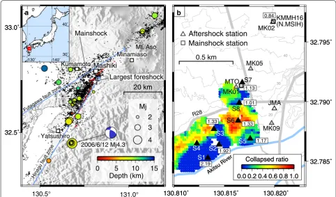
part of Kumamoto Prefecture, southwestern Japan, and caused severe damage in areas between Kumamoto City and Minamiaso Village near the Futagawa and Hinagu fault zones (see the locations in Fig. 1a). Significant sur-face ruptures associated with the earthquake sequence appeared in Mashiki Town, which is located at the junc-tion of the two major fault zones (Shirahama et al. 2016; Sugito et al. 2016; Toda et al. 2016) and seismic intensity of 7, the maximum seismic intensity scale of the Japan Metrological Agency (JMA), was measured during both larger events. The results of damage investigations (e.g., National Institute for Land and Infrastructure Manage-ment and Building Research Institute 2016; Sugino et al.
2016b; Tomozawa et al. 2017; Yamada 2017; Yamada et al.
2017a, b) showed that heavily damaged buildings were concentrated in a narrow region between Kumamoto Prefectural Route 28 (R28) and the Akitsu River running from east to west in the central part of Mashiki (Fig. 1b).
Field surveys after the mainshock also showed that the cause of the varying damage distribution could be explained by different site conditions of this area. According to the landform classification map for flood control published by the Geospatial Information Author-ity of Japan, the distribution of damaged buildings cor-responds well to the river terrace between R28 and the Akitsu River, whereas almost no buildings collapsed in the floodplain and old river channel along the Akitsu riverside (e.g., Yamada 2017; Yamada et al. 2017a, c). These findings indicate that the building damage pat-tern is strongly affected by the site conditions associated with local subsurface geology. The results of single-point
32.5˚
microtremor observations in this area (e.g., Kagawa et al.
2017; Kawase et al. 2017; Nagao et al. 2017) showed a clear correlation between the patterns of peak frequency in the horizontal-to-vertical (H/V) spectral ratios and the landform characteristics. Yamada et al. (2017c) per-formed further microtremor observations with miniature arrays at 108 sites in Mashiki and clarified the differences of Rayleigh wave dispersion characteristics between the damaged and undamaged zones. They found that an extremely low S wave velocity (Vs) layer (< 100 m/s) exists at very shallow depth beneath Mashiki. The estimated thickness of this layer is less than several meters in the severely damaged zones, where the dominant frequencies of microtremor H/V spectral ratio are higher than 2 Hz. In contrast, in the floodplain of the Akitsu River where almost no buildings were collapsed, the low-velocity layer is thicker than 10 m and the dominant H/V frequencies were around 1 Hz.
The predominant frequency of soil layers is funda-mental information in seismic microzonation and a rea-sonable indicator that relates the local site condition to earthquake damage. Past observations of damaging earthquakes in Japan showed that the strong ground motions in the frequency range between 0.5 and 1 Hz greatly affect wooden buildings (e.g., Kitagawa and Hirai-shi 2004; Sakai et al. 2008). The natural frequency of low-rise wooden buildings is between 2 and 10 Hz (e.g., Sugino et al. 2016a), but the frequency may shift to lower values (around 1 Hz) when they are subjected to strong shaking. Therefore, larger damage was expected along the Akitsu river where the frequencies around 1 Hz are dominant. However, the damage investigations showed very different results with relatively light damage close to the river and more severe damage associated with sites of higher natural frequencies that were located farther from the river. Besides the local differences in site conditions, there are several other possible factors that could account for the damage concentration in Mashiki; the construc-tion years of buildings (e.g., Mori et al. 2017; Sugino et al.
2016b; Yamada 2017), types of foundations in the build-ings (e.g., Mori et al. 2017), and/or surface fault ruptures (e.g., Suzuki et al. 2016). There were no strong-motion records of the larger events in the heavily damaged zones so that aftershock data recorded in both the damaged and undamaged zones are used to help understand the difference of seismic response.
Recent studies have tried to explain this unusual site amplification in Mashiki using nonlinear site response analyses, assuming that frequencies between 0.5 and 1 Hz were dominant in the heavily damaged zones and lower frequencies were dominant in the less damaged zone. Yamada et al. (2017c) calculated the seismic response for both damaged and undamaged zones of Mashiki using
shallow seismic velocity structure models obtained from microtremor observations with typical nonlinear proper-ties of sand and clay. Shingaki et al. (2017) and Yoshimi et al. (2017) determined dynamic properties of surface soils including volcanic ash clay, using actual soil sam-ples in Mashiki, and Nakagawa et al. (2017) performed time-history response analysis for the mainshock at two sites in Mashiki using the obtained dynamic deforma-tion properties. For analyzing the ground modeforma-tions of the mainshock, information from the borehole (252 m in depth) of the closest KiK-net strong-motion observation station, KMMH16 (see the location in Fig. 1b) was used. The station is operated by the National Research Institute for Earth Science and Disaster Resilience (NIED) and located about 1 km to the northeast of the severely dam-aged area. Velocity models obtained from the borehole logging are well constrained for the shallower depths (less than a few tens of meters) but have lower resolution for the deeper structure. Therefore, it is important to evalu-ate the deep sedimentary structure in the damaged area.
To investigate the differences of ground motion charac-teristics in the heavily and less damaged zones as well as station KMMH16, we conducted aftershock and micro-tremor (ambient noise) observations in and around the damaged zones of Mashiki (see the observation locations in Fig. 1b). Figure 1b also shows the locations of after-shock observation stations deployed by Yamanaka et al. (2016) (gray triangles: MK01, MK02, MK05 and MK09) and a seismic intensity station deployed by JMA (white triangle) just after the mainshock. Our aftershock obser-vation sites were installed in the heavily damaged zones, while the existing temporary aftershock stations were located outside of this zone. In this paper, we show the differences of the ground motion characteristics between the contrasting zones and propose a velocity structure model of the entire area for seismic response analysis. Field observations
The aftershock and microtremor observations were con-ducted from June 10 to June 13, 2016, 2 months after the mainshock. Dimensions of the observation area are approximately 500 m in the east–west direction and 750 m in the north–south direction, which corresponds to the area of our damage and microtremor surveys (Yamada et al. 2017a, c). This area is a fluvial terrace of the Akitsu River and the altitude increases as a function of distance toward the north from the river. We installed eight accelerometers in and around the damaged zones at intervals of approximately 150–200 m (S1–S8: see Table 1
MTO. We used JEP-6A3 (Mitsutoyo Corp.) over-damped accelerometers at sites S1–S4, and SMAR-6A3P (Mit-sutoyo Corp.) over-damped accelerometers at the other sites. Each sensor was connected to a 24-bit data logger DATAMARK LS-8800 (Hakusan Corp.), with a sampling frequency at 200 Hz. All the sensors were installed on the ground surface, outside of buildings and power was supplied from external batteries. Both types of sensors have the same response characteristics, except different sensitivities (0.112 V/m/s2 for JEP-6A3 and 0.224 V/m/s2
for SMAR-6A3P). The pretests confirmed that all of the sensors have the correct frequency response to an input signal between 0.2 and 10.0 Hz for both horizontal and vertical components.
We distributed the sensors in areas with different building damage ratios; sites S1 and S2 were located in a zone with no collapsed buildings near the Akitsu riv-erside, and the other sites were located in the damaged zones. Figure 1b also shows the ratio of the totally col-lapsed wooden buildings that correspond to damage grade D5 (story failure) in the damage scale proposed by Okada and Takai (1999). The sensor at site S6 was deployed at a location where 77% of the wooden build-ings were collapsed. The distance between site S7 and the station MTO was about 30 m so that we will discuss the ground motion differences between the mainshock observation station and the other temporary stations in the latter part. We excluded the data at site S4 in the following analyses due to a possible problem in the sen-sor cable, although signals related to earthquake ground motions were recorded.
We also used data from the surface and borehole com-ponents of KiK-net station KMMH16 and co-located Hi-net station M.MSIH. We confirmed that the frequency responses from 0.14 to 20 Hz were very consistent for the two instruments in the borehole (see an example in Addi-tional file 1: Fig. S1).
Results
Aftershock data on July 12, 2016
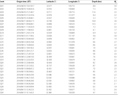
Earthquake ground motion data from the after-shocks were manually extracted from the continuously recorded waveforms, based on the unified earthquake catalogue provided by JMA. We selected events with maximum JMA seismic intensity in the Kumamoto Pre-fecture higher than or equal to 1. Ground motion data from 30 events with clear P- and S wave signals were obtained (see the event information in Table 2 and the hypocenter distribution in Fig. 1a). Epicenters of the aftershocks are in the regions correspond to the mid-dle and northern sections of the Hinagu fault zone, the west part of the Futagawa fault zone and the north side of Mt. Aso. The JMA magnitude (Mj) of the selected
events ranged from 1.7 to 4.3 and the depths were rela-tively shallow (between 1.9 and 13.5 km).
The largest event with Mj 4.3 (MW 4.2; EQ18 in Table 2)
occurred in the southern Yatsushiro City (see the hypo-central location in Fig. 1a) at 22:08 JST on June 12. JMA seismic intensity 5-lower was measured nearby Saka-moto, Yatsushiro City. This event was one of the three events from April 20, 2016, to the present time (June 2018) with maximum JMA seismic intensity larger or equal to 5-lower in Kumamoto Prefecture. Epicentral distance from Mashiki is about 40 km, and JMA seismic intensity of the event was 1 at MTO. Figures 2 and 3 show the observed accelerograms and Fourier amplitude spec-tra of the Mj 4.3 recordings at the observation sites S1–S8
except S4, together with those for the surface and bore-hole components of KiK-net station KMMH16. In Fig. 2, the accelerograms recorded at sites S1 and S2 clearly show the long period components and long duration with large amplitude in the horizontal components. The Fou-rier amplitude spectra at sites S1 and S2 have dominant peaks around 1 Hz in the horizontal components which are not seen at other sites (Fig. 3).
Table 1 Temporary stations for aftershock observation of the 2016 Kumamoto earthquake
a From the Denshi-kokudo web system (https ://maps.gsi.go.jp/) provided by the Geospatial Information Authority of Japan
b Observed data at site S4 were not used in this study
Site Latitude (°) Longitude (°) Altitudea (m) Start End
S1 32.78533 130.81335 11 2016/06/10 15:51 2016/06/13 13:01
S2 32.78636 130.81449 11 2016/06/10 15:13 2016/06/13 13:34
S3 32.78774 130.81398 14 2016/06/10 14:23 2016/06/13 13:17
S4b 32.78655 130.81231 12 2016/06/10 17:30 2016/06/13 13:50
S5 32.78692 130.81761 12 2016/06/10 17:30 2016/06/13 13:01
S6 32.78837 130.81638 19 2016/06/10 16:30 2016/06/13 13:15
S7 32.79157 130.81685 33 2016/06/10 14:25 2016/06/13 13:44
Characteristics of the site amplifications
Figure 4 shows the spectral ratios of the S wave (20.48 s segment from the S wave onsets) between our surface observation sites and the borehole station M.MSIH, for all the detected events. A cosine taper was applied to both sides of the S wave segments with a 5% width of the segment time length. Assuming that the input ground motions beneath our observation area and KMMH16 station are similar and the S wave is dominant in the segments, the spectral ratios represent the approximate borehole to surface S wave transfer functions of subsur-face layers at each site. The shapes of the derived spec-tral ratios look slightly different between the NS and EW components at some sites possibly due to the complex velocity structure, but there are no significant differences in the dominant peak frequencies. The spectral ratios clearly show dominant peaks around 1–2 Hz at sites
S1 and S2 with amplitudes greater than 20, while other sites show peaks at higher frequencies (> 3 Hz). This is consistent with the results of past microtremor surveys which showed site amplifications at around 1 Hz near the Akitsu River (Kawase et al. 2017; Nagao et al. 2017; Yam-ada et al. 2017c).
Next, we obtained H/V spectral ratios at each obser-vation site from the ambient noise sections of the recordings. The derived probability density functions for our continuous data show the measurable frequency range of microtremor down to 0.2 Hz (see an example in Additional file 1: Fig. S2). We selected 1-h continu-ous waveform data during a quiet period of the 4-day continuous records (between 0:00 and 1:00 JST on June 11). The three-component recordings were divided into 40.96 s window segments with 50% overlap, and fast Fourier transforms were applied to each segment. Then, Table 2 List of the detected events
From the unified earthquake catalog provided by JMA
Event Origin time (JST) Latitude (°) Longitude (°) Depth (km) Mj
EQ01 2016/06/10 15:41:59.7 32.577 130.715 8.6 3.0
EQ02 2016/06/10 15:44:43.6 32.555 130.669 7.3 2.5
EQ03 2016/06/10 21:21:48.7 32.711 130.715 11.6 2.2
EQ04 2016/06/10 21:32:29.6 32.976 131.077 8.4 2.2
EQ05 2016/06/10 23:38:48.1 32.557 130.649 2.2 1.7
EQ06 2016/06/11 04:58:27.3 32.740 130.606 10.8 2.8
EQ07 2016/06/11 09:56:08.1 32.806 130.525 13.5 3.1
EQ08 2016/06/11 11:59:34.9 32.553 130.662 7.2 3.3
EQ09 2016/06/11 17:08:34.3 32.801 130.720 6.1 1.7
EQ10 2016/06/11 23:41:27.8 32.559 130.669 6.9 3.2
EQ11 2016/06/12 01:17:49.2 33.056 131.147 9.6 3.0
EQ12 2016/06/12 03:56:54.0 32.694 130.802 8.7 1.9
EQ13 2016/06/12 04:35:16.8 32.982 131.078 8.4 2.7
EQ14 2016/06/12 15:58:43.0 32.643 130.693 8.4 2.2
EQ15 2016/06/12 19:47:45.3 32.591 130.681 1.9 1.8
EQ16 2016/06/12 20:31:21.7 32.655 130.695 8.6 2.2
EQ17 2016/06/12 21:20:13.9 32.801 130.672 9.4 2.5
EQ18 2016/06/12 22:08:15.0 32.449 130.681 7.4 4.3
EQ19 2016/06/12 22:53:29.3 32.450 130.679 7.4 3.1
EQ20 2016/06/12 23:08:30.6 32.654 130.693 8.2 2.6
EQ21 2016/06/12 23:12:55.2 32.737 130.628 8.7 2.8
EQ22 2016/06/13 00:00:41.2 32.451 130.679 7.5 2.2
EQ23 2016/06/13 00:39:04.2 32.663 130.721 8.5 2.5
EQ24 2016/06/13 04:03:29.0 32.646 130.671 9.6 2.2
EQ25 2016/06/13 04:21:35.0 32.632 130.686 6.8 2.1
EQ26 2016/06/13 04:46:28.0 32.633 130.682 6.8 2.2
EQ27 2016/06/13 09:26:28.0 32.450 130.676 7.0 2.1
EQ28 2016/06/13 09:39:09.9 32.803 130.705 6.3 1.8
EQ29 2016/06/13 12:34:22.5 32.452 130.677 7.2 2.6
the H/V ratios were computed and smoothed using a Parzen window with bandwidth of 0.1 Hz, and all the ratios were stacked together. Note that we removed seg-ments with large amplitude irregular noise in advance and the total number of segments used for the analy-sis was more than 140 for each site. Figure 5 shows the derived microtremor H/V ratios, as well as the spectral
ratios of the north–south and east–west horizontal components with the vertical component (NS/V and EW/V, respectively) at all observation sites. The derived spectral ratios indicate predominant peaks in the fre-quency around 1–2 Hz at sites S1 and S2, where there was no building damage. This feature is consistent with the surface/borehole spectral ratios derived from our aftershock data. The trend in the dominant frequency
NS EW UD
0 20 40 60
Time [s]
4
-4
cm/s
2
0 20 40 60
Time [s] 0 20 Time [s] 40 60
4.03
3.25
2.08
2.73
2.61
2.26
2.21
2.12
0.30
5.10
5.41
3.41
2.84
3.40
2.86
1.42
2.05
0.27
2.84
1.58
1.11
1.02
1.28
1.74
0.75
1.65
0.17 S1
S2
S3
S5
S6
S7
S8
KMMH16 (surface)
KMMH16 (borehole)
Fig. 2 Three-component acceleration waveforms recorded at temporary observation sites and KiK-net station KMMH16 during event EQ18. The peak ground acceleration (cm/s2) values are denoted at the upper right-hand side of each trace
101
100
10-1
10-2
10-3
0.2 0.5 1 2 5 10
Frequency [Hz]
NS
EW
UD
S1 S2 S3-S8 KMMH16 (surface)
cm/s
0.2 0.5 1 2 5 10
Frequency [Hz]
0.2 0.5 1 2 5 10
Frequency [Hz]
0.1 1 10 100
Spectral ratio
0.2 0.5 1 2 5 10
Frequency[Hz]
0.1 1 10 100
0.2 0.5 1 2 5 10
Frequency[Hz]
0.1 1 10 100
0.2 0.5 1 2 5 10
Frequency[Hz]
0.1 1 10 100
Spectral ratio
0.2 0.5 1 2 5 10
Frequency[Hz]
0.1 1 10 100
0.2 0.5 1 2 5 10
Frequency[Hz]
0.1 1 10 100
0.2 0.5 1 2 5 10
Frequency[Hz]
0.1 1 10 100
0.2 0.5 1 2 5 10
Frequency[Hz]
S1 S2 S3
S5 S6 S7 S8
surface/borehole(NS) surface/borehole(EW)
Fig. 4 Fourier spectral ratios between each temporary aftershock observation site and Hi-net station N.MSIH for all detected events. Blue and red traces show the ratios for the S wave portions from NS and EW components, respectively. Thin traces show the spectral ratios derived for each event and thick traces corresponds to the median values. Note that the sampling frequencies at the temporary sites have been reduced to 100 Hz
0.1 1 10 100
Spectral ratio
0.2 0.5 1 2 5 10 Frequency[Hz]
0.1 1 10 100
0.2 0.5 1 2 5 10 Frequency[Hz]
0.1 1 10 100
0.2 0.5 1 2 5 10 Frequency[Hz]
0.1 1 10 100
Spectral rati
o
0.2 0.5 1 2 5 10 Frequency[Hz]
0.1 1 10 100
0.2 0.5 1 2 5 10 Frequency[Hz]
0.1 1 10 100
0.2 0.5 1 2 5 10 Frequency[Hz]
0.1 1 10 100
0.2 0.5 1 2 5 10 Frequency[Hz]
S1 S2 S3
S5 S6 S7 S8
Microtremor H/V Microtremor NS/UD Microtremor EW/UD
Earthquake R/V (EQ18)
is also comparable with the results of single-station microtremor H/V spectral ratios (Yamada et al. 2017c).
We also derived earthquake radial-to-vertical (R/V) spectral ratios using the data of event EQ18 (Mj 4.3 and
MW 4.2) that contain surface waves in the coda. After
rotation of the two horizontal components (NS and EW) to radial and transverse components with respect to each source-sensor azimuth, we selected 20.48 s segments from 10 s after the S wave arrivals. The spectral ratios of radial-to-vertical motions that would correspond to Rayleigh wave ellipticity were computed at each site. Here, the same smoothing filter as the microtremor H/V calculations above was applied. Figure 5 also shows the derived earthquake R/V ratios at each observation site. They show peak frequencies similar to the H/V spec-tra and the predominant peaks (ratios of 30 or greater) around 1–2 Hz are also seen at sites S1 and S2. The peaks at 1–2 Hz are also recognized at sites S3, S5, S6 and S8, but the ratios are substantially smaller (between 5 and 20) compared to those in the less damaged zone and other predominant peaks with larger values are seen at the higher frequency range (> 2 Hz).
Besides the predominant peaks at frequencies higher than 1 Hz, there are distinct peaks at 0.4 Hz for all the spectra, especially at S5–S8. This peak can also be observed in the microtremor H/V spectra with smaller amplitudes. The common dominant peaks of the micro-tremor H/V and earthquake R/V ratios at this lower frequency are possibly related to the response of deep sedimentary layers beneath the area, which will be dis-cussed in a later section.
Rayleigh wave phase velocity
We estimated dispersion characteristics of Rayleigh wave phase velocities in the lower frequency range using con-tinuous microtremor and event data. We applied the two-site SPAC (2sSPAC) method (e.g., Morikawa et al.
2004; Hayashi et al. 2013) for the microtremor data, assuming that the microtremor wave-field around the area is spatially and temporally uniform. We selected four sensor pairs around the heavily damaged zones (S6–S8: 167 m, S5–S8: 201 m, S3–S6: 238 m, and S3–S5: 349 m) for the data processing. We used the vertical compo-nent of microtremors recorded during the entire obser-vation period (from June 10, 18:00 to June 13, 13:00). At first, 1-h continuous data were divided into 87 segments (time window of 40.96 s) without overlap. After removal of segments containing irregular noise or earthquake signals, fast Fourier transforms were performed on the datasets and the complex coherence functions between the selected site-to-site pairs were calculated. The coher-ence functions from all the segments were stacked and an hourly stacked coherence function was derived. If an
hourly derived coherence function showed small values around 1 Hz in comparison with many other traces, indi-cating small coherence between the two datasets, those data were excluded. Finally, all the hourly derived coher-ence functions were summed and the averaged function (with the variance) was regarded as the SPAC coefficients for the sensor pair. The Rayleigh wave phase velocities were estimated from the derived SPAC coefficients using a fifth-degree polynomial that approximates the inverse function of the zero order Bessel function of the first kind. The frequency range we used for the determination of phase velocity depended on the sensor distance; it is determined so that the wavelength corresponding to the estimated phase velocity was 2–7 times the sensor dis-tances. The estimated phase velocity dispersion curves from the four sensor-to-sensor pairs were combined to derive a single dispersion curve. Since each SPAC coef-ficient curve has the variance so that the dispersion curve has been derived by the inverse-variance weighted method. The coherence functions of microtremors are not always stable in the lower frequency band due to the low detection performances and the final accepted fre-quency range for the 2sSPAC analysis was between 0.98 and 1.27 Hz (Fig. 6a).
We also estimated the Rayleigh wave phase veloci-ties from aftershock data (event EQ18) based on the semblance analysis of the S-coda wave (Fukumoto et al.
2004), assuming that the coda wave is dominated by sur-face waves. The phase velocities were estimated at fre-quencies from 0.2 to 0.9 Hz with an interval of 0.01 Hz, using narrow-band velocity waveforms (0.9 and 1.1 times the target frequency for the low-frequency and the high-frequency cutoffs, respectively) in the vertical compo-nent. The length of the time window for the analysis is twice the reciprocal of the target frequency, and the win-dow was shifted every 0.5 s throughout the dominant wave train. For each time window, the apparent veloc-ity as well as incident angle was calculated. The derived apparent velocities with sufficient semblance values (≥ 0.9) were averaged, and the phase velocity for each fre-quency was determined.
our phase velocity results. For the semblance analysis, we obtained dispersive characteristics of phase velocities in the frequency range between 0.24 and 0.86 Hz. The esti-mated phase velocities from microtremor and event data also show similar continuous characteristics for the com-mon frequency range, suggesting that our estimations are reasonable.
S wave velocity structure model beneath KiK‑net station KMMH16
We refined the P–S logging model at the closest KiK-net station KMMH16 (see Table 3 and Fig. 6b) by using our
dispersion curve of Rayleigh wave phase velocity. We performed velocity structure inversions using a genetic algorithm (GA) technique (Yamanaka and Ishida 1996) to obtain a velocity structure model that can explain the estimated Rayleigh wave dispersion curve.
There are several previous velocity structure models in this area. The P–S logging model at KiK-net station KMMH16 has information down to 252 m depth. Goto et al. (2016) tuned the KiK-net logging model (hereinaf-ter called GOTO model; see Table 3) using the surface/ borehole spectral ratio of the small event data. They inverted for Vs values of the top five layers to fit the
a
b
d
c
0 500 1000 1500 2000 2500 3000
Phase velocity [m/s]
0.2 0.5 1 2 5 10
Frequency [Hz]
0
300
600
900
1200
1500
Depth [m
]
0 1000 2000 3000 Vs [m/s]
PS logging GOTO J−SHIS SIP2017 This study
0 500 1000 1500 2000 2500 3000
Phase velocity [m/s]
0.2 0.5 1 2 5 10
Frequency [Hz]
0.1 1 10 100
H/
V
0.2 0.5 1 2 5 10
Frequency [Hz] S1
S6 S7 KMMH16
surface/borehole spectral ratio, and used 75% of the Vs in the logging model for the 6th–12th layers due to the limited sensitivity to the deeper structure (Table 3). For deeper structures, the Seismic Hazard Informa-tion StaInforma-tion of NIED (J-SHIS: http://www.j-shis.bosai .go.jp) provides a nationwide velocity model based on the borehole logging, reflection and gravity surveys. In the J-SHIS model, the velocity structure beneath the target area consists of six layers; three subsurface layers (600 m/s ≤ Vs ≤ 2100 m/s) along with three upper
crus-tal layers (3100 m/s ≤ Vs ≤ 3400 m/s). Figure 6c shows the
theoretical dispersion curves obtained from the KiK-net logging data, GOTO and J-SHIS models, respectively. The KiK-net P–S logging model clearly overestimates the Rayleigh wave velocity for almost the entire fre-quency range, suggesting the actual Vs values are much lower than those of the logging model. The GOTO model explains the dispersion curve reasonably well at the higher frequency range (3–10 Hz) that corresponds to the target frequency range of miniature microtremor survey at the site (Yamada et al. 2017c), but still under-estimates the lower frequency range even after the 75% reduction of Vs. The observed dispersion curve in Fig. 6c suggests that the hard rock layer (Vs > 3000 m/s) as in the J-SHIS model is necessary to explain the low-frequency range of the dispersion curve.
We constructed an initial model for the GA in the fol-lowing procedure. We directly use the GOTO model for
the top five layers, since the theoretical dispersion curve explains the observed dispersion curve at the higher fre-quency range. We also use the GOTO model as the start-ing model for the 6th–12th layers in the inversion. Due to the uncertainty of the deeper structure, we use the thick-nesses and Vs values of the J-SHIS model for the layers of bedrock (Vs ≥ 2700 m/s). In the preliminary analysis,
we found that the Vs = 2700 m/s layer in the P–S
log-ging model (234 m) is too shallow to explain our disper-sion curve. Therefore, we assumed that the layer would be deeper than the depth of the borehole. Based on this assumption, we modified the properties of the 13th layer in the GOTO model to those of the 12th layer, and added an extra layer (Vs = 1470 m/s) underneath the borehole
with an unknown depth.
In total, we have 18 layers for our initial velocity model: the 1st–5th layers of the GOTO model, 6th–13th layers of the GOTO model for which Vs values will be deter-mined, 14th layer with Vs = 1470 m/s with unknown
thickness, and four bedrock layers of the J-SHIS model with Vs = 2700–3400 m/s at the bottom (Table 3). Since
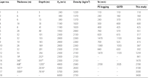
there is a trade-off between Vs and thickness of layers, we fix the thickness for the 1st–13th layers and the Vs for the 14th layers just above the bedrock. Other observa-tions such as receiver funcobserva-tions might reduce trade-offs between the velocity and thickness of each layer; however, the small events (M3 and smaller) in our dataset were not appropriate for this method. Therefore, we validate Table 3 Seismic velocity structures at KiK-net Mashiki station (KMMH16)
a Parameters only for the optimized velocity model in this study
Layer no. Thickness (m) Depth (m) VP (m/s) Density (kg/m3) Vs (m/s)
PS logging GOTO This study
1 3 3 240 1220 110 110 110
2 6 9 380 1370 240 160 160
3 6 15 380 1370 240 370 370
4 18 33 1180 1820 500 600 600
5 8 41 1180 1820 400 425 425
6 28 69 1950 2060 760 570 551
7 32 101 2300 2150 820 615 517
8 32 133 2800 2260 1470 1103 564
9 10 143 2800 2260 700 525 415
10 26 169 2800 2260 1380 1035 587
11 32 201 2300 2150 840 630 392
12 33 234 2300 2150 1470 1103 1239
13 18a 252a 2300 2150 – – 841
14 345a 597a 2300 2150 – – 1470
15 608a 1205a 4800 2580 2700 2025 2700
16 1411a 2616a 5360 2650 – – 3100
17 5000a 7616a 5700 2690 – – 3300
the reliability of the inversion results focusing on the predominant frequency of the theoretical microtremor H/V, as well as the travel-times of body waves between the ground surface and borehole sensor depth in com-parison with the GOTO model. The determined param-eters for the inversion are Vs values of eight layers and thickness of the 14th layer; the range of the parameter search for Vs is ± 50% of the initial value, and 0–1024 m for the thickness. Since there is no available information on the density profile at station KMMH16, we assigned the parameters based on the relation between Vp and density (Gardner et al. 1974). In the GA optimization, the number of generations that corresponds to the total number of iteration is 500 and the number of population in each generation is 30. Crossover and mutation rates were set to 0.5 and 0.01, respectively. We repeated this optimization process twice by setting the output of the first process as an input of the second process, so that the most optimal values are inside of the range of the param-eter search. We used a subroutine program package DIS-PER80 (Saito 1988) to compute the theoretical dispersion curves for the generated models.
The optimal velocity profile is shown in Fig. 6b and Table 3 with the phase velocities of Rayleigh wave, and theoretical H/V ratios are shown in Fig. 6c, d, respec-tively. The estimated values for Vs at the 6th–13th layers are substantially smaller than those of the logging model and GOTO model. The estimated depth of the bedrock layer is about 600 m. The comparisons of H/V ratios and phase velocities show that the agreements between the theoretical and estimated phase velocities are sub-stantially improved. Also, the H/V spectral peak around 0.4 Hz is reproduced well by our model, which does not
appear in the theoretical H/V spectra of the P–S logging model and GOTO model. Based on the quarter wave-length law, this peak reflects the velocity contrast of the bedrock, suggesting that the bedrock depth can be much deeper than the logging data (234 m).
Discussion
Earthquake damage and site amplification
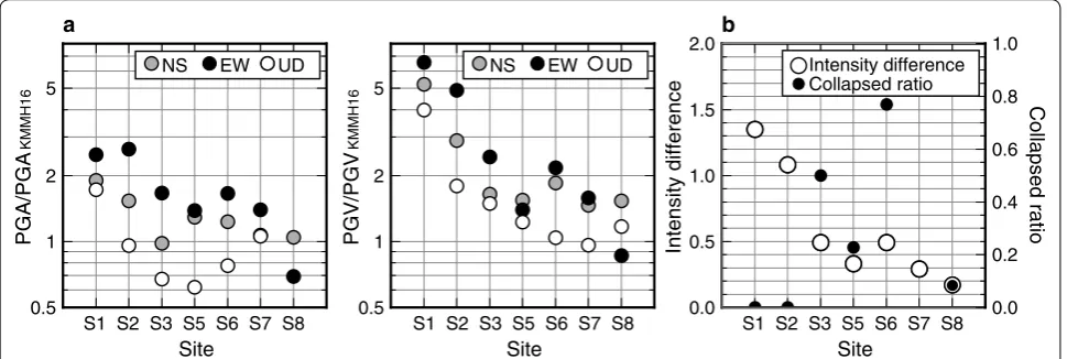
We discuss the relationship between the damage dis-tribution and the largest aftershock (EQ18) during our observation period. For various ground motion meas-ures, Fig. 7a, b shows the ratios of the peak ground accel-eration (PGA) and peak ground velocity (PGV), and the differences of the JMA seismic intensity values between our observation sites and the KiK-net KMMH16 sur-face station (actual seismic intensity values are shown in Fig. 1b), respectively. Figure 7b also shows the ratios of the totally collapsed wooden buildings within 50 m radius at each site. Note that site S7 was located inside the town office where there were no houses nearby and the damage ratio was not available. This also shows that the ground motions of EQ18 are larger than those at other sites at sites S1 and S2 where there were no collapsed buildings around the sensors sites during the largest foreshock and mainshock. Figure 8 shows the acceleration response spectra for the EW component using the data of EQ18 at sites S1, S2, S6, S7 and KMMH16 together with the geo-metrical mean of the spectra (sites S1–S3, S5–S8). This clearly indicates that the different site response between the minimally damaged zone (S1 and S2) and the severely damaged zones (S6) as well as site nearby MTO (S7) and station KMMH16, and that the larger response at around 1 Hz can be seen only in the less damaged zone.
0.5 1 2 5
PGA/PGA
KMMH16
Site
a
0.5 1 2 5
PGV/PGV
KMMH16
Site
0.0 0.5 1.0 1.5 2.0
Intensity difference
Site
0.0 0.2 0.4 0.6 0.8 1.0
Collapsed ratio
b
S1 S2 S3 S5 S6 S7 S8 S1 S2 S3 S5 S6 S7 S8 S1 S2 S3 S5 S6 S7 S8
NS EW UD
NS EW UD Intensity difference
Collapsed ratio
As we expected from microtremor geotechnical sur-veys, our aftershock data show that ground motions around 1 Hz were amplified on the floodplain of the Akitsu River, while the amplification of this frequency range is much less in the damaged zone. This observa-tion is inconsistent with the damage distribuobserva-tion of the mainshock, which shows severe damage away from the river. We need to consider other mechanisms, such as nonlinear site amplification, to explain the strong ground motions in Mashiki.
Comparisons of the velocity model with existing models We determined a subsurface Vs structure model above the seismic bedrock with the derived dispersion curves of Rayleigh-wave phase velocities from our 4-day obser-vation data in the entire area and miniature microtremor array at KiK-net station KMMH16. We assumed that the deep sedimentary layers for the damaged area are the same as in the vicinity of station KMMH16. If the assumption is correct, the dominant peak around 0.4 Hz in the earthquake R/V spectral ratios that corresponds to the velocity contrast at the seismic bedrock, should be seen in the KMMH16 data. Figure 9 shows R/V spectral ratios at station KMMH16 computed from the 19 shal-low crustal earthquakes (> M4) that occurred prior to the 2016 Kumamoto earthquake (see the earthquake lists in Table 4). The length of the time window and the band-width for smoothing is the same as the R/V analysis. This
averaged spectrum also shows the peak at 0.4 Hz, which suggests that the velocity contrast should exist over a relatively wide area, at least across the area of our after-shock observations and the KiK-net KMMH16 station.
We would like to compare our velocity model to other existing models. In the nationwide J-SHIS model, the depth of the bottom of the subsurface layers is 602 m, which is consistent with our estimation. Since the shal-lower part of the structure with low Vs (< 600 m/s) is not included in the J-SHIS model, the shallow veloc-ity was greatly overestimated and the computed dis-persion curve of Rayleigh waves beneath Mashiki has a large discrepancy with our observed dispersion curve (Fig. 6c). Also, the peak in the H/V spectrum at 0.4 Hz could not be explained (Fig. 6d). A group in NIED con-ducted microtremor observations with large-sized arrays after the Kumamoto earthquake and constructed a three-dimensional (3D) structure model of the deep sedimentary layers (Ogawa et al. 2017; Senna et al. 2017a,
b). In their model (hereinafter called SIP2017 model), the velocity structure consists of five subsurface lay-ers (350 m/s ≤ Vs ≤ 2100 m/s) and the bedrock layer (Vs = 2700 m/s) that was not included in the J-SHIS model. The velocity profile, theoretical H/V ratio, and dispersion curve of Rayleigh wave phase velocity com-puted from the SIP2017 model are shown in Fig. 6b–d, respectively. The depth to the bedrock layer in the SIP2017 model is much deeper than the P–S logging
Spectral cceleration (cm/s
2)
0 5 10 15 20 25
0.1 1 10
Period (s)
S1
S2
S6
S7
KMMH16
Fig. 8 Acceleration response spectra with 5% of damping ratio derived from recordings of event EQ18 in Mashiki. Yellow, purple, blue and red traces indicate the response spectra at sites S1, S6, S7 and KMMH16. Dashed line shows the geometric mean of the response spectra derived using observed accelerograms at S1–S3 and S5–S8
0.1 1 10 100
R/V
0.2
Frequency[Hz]
10 5
2 1
0.5
model and the consistency between the estimated and theoretical phase velocity characteristics are reasonable in comparison with the J-SHIS model, although the peak frequency of the theoretical H/V is slightly higher than that of our observations. Our velocity model calibrated by the existing Vs profile at the KiK-net KMMH16 site (Goto et al. 2016) and dispersion curve of Rayleigh wave phase velocity can explain the H/V peak reasonably well. In the SIP2017 model the depth to the Vs = 2700 m/s layer (1417 m) is much deeper than our estimation but the depth of the high-Vs layer (Vs = 2100 m/s) above the bedrock layer (597 m), which was not included in our model, is very close to our estimated bedrock depth, indi-cating that the difference in starting structure models for inversions produced different solutions for the bedrock depth. The exact depth of the bedrock for this area is still controversial, but at least both observations suggest that the depth of Vs > 2000 m/s layer is much deeper than that of the KiK-net logging data (234 m) and is expected to be about 600 m. Our aftershock data and velocity model help improve knowledge of the deep sedimentary struc-ture model in this area.
Conclusions
We conducted aftershock and microtremor observations at eight sites in and around the damaged areas in Mashiki Town, Kumamoto Prefecture, 2 months after the 2016
Kumamoto earthquakes. The aftershock data indicate that site amplifications at approximately 1 Hz are sig-nificant during the small events in the less damaged zone where a thick low-velocity surface layer exists, whereas the dominant frequencies are higher than 3 Hz in the damaged zones. These trends are similar to the results from microtremor surveys in the area, indicating that the characteristics of ground motions for the mainshock and small earthquakes show opposite trends in Mashiki. Our observations support the idea that the dominant frequen-cies of the heavily damaged area were shifted to 1–2 Hz which has a great effect on wooden buildings during the largest foreshock and mainshock, while in the less dam-aged zone, the 1–2 Hz peaks would be shifted to much lower frequency range, which had less effect on the build-ings. The estimated phase velocities of Rayleigh wave using microtremor data as well as the aftershock data (EQ18) are smaller than those of the P–S logging model at the KiK-net station KMMH16. The derived micro-tremor H/V and earthquake R/V ratios from our data show common dominant peaks around 0.4 Hz, which is possibly related to the response of deeper structure beneath the observation area. We performed a GA inver-sion for the deep sedimentary structure model with the derived phase velocities and the dominant frequency peaks to estimate an optimal structure model near sta-tion KMMH16. The estimated velocity structure model indicates that the Vs values at shallower depths in the target area are substantially smaller compared to exist-ing models. Also, the depth to the bedrock layer might be much deeper (about 600 m), in comparison with the existing model from logging data (234 m). The earth-quake R/V spectral ratios at station KMMH16 also show the common peak at 0.4 Hz, suggesting that the similarity of deeper structures between the KiK-net station and our observation area in the severely damaged zone. There-fore, mainshock data recorded in the borehole at station KMMH16 could be directly used as input motions for seismic response analysis in the damaged zone.
Additional file
Additional file 1. Fig.S1: Observed accelerograms and Fourier amplitude spectra at KiK-net KMMH16 and Hi-net N.MSIH stations. a Compari-sons of the observed three-component acceleration records, b Fourier amplitude spectra at KiK-net borehole station KMMH16 (black traces) and Hi-net station N.MSIH (red traces) for event EQ18. Note that the original velocity seismograms observed at N.MSIH have been differentiated after the removal of instrumental responses. Fig. S2: Four-day long power spectral density of the recorded seismic noise at site S6. Here the power is expressed as decibel (dB), which corresponds to 10log10(m2/s4/Hz) of spectral acceleration.
Table 4 Events used for calculation of earthquake R/V ratios at station KMMH16
From the unified earthquake catalog provided by JMA
Origin time (JST) Latitude (°) Longitude (°) Depth (km) Mj
Authors’ contributions
TH, MY1, JM, MY2 and KH planned the survey, and TH, MY1, MY2, KH, JM, YF, HS, SF, EN, TO and AF participated in the observations. TH analyzed the observed data and MY1 performed velocity structure inversions. TH, MY1, MY2, KH, JM and YF contributed to interpretations of the results. TH wrote the initial draft of the manuscript and MY1 and JM edited it. All authors read and approved the final manuscript.
Author details
1 International Institute of Seismology and Earthquake Engineering, Building Research Institute, 1 Tachihara, Tsukuba, Ibaraki 305-0802, Japan. 2 Disaster Prevention Research Institute, Kyoto University, Gokasho, Uji, Kyoto 611-0011, Japan. 3 The New Japan Engineering Consultants Incorporated, 2-3-20 Honjo-Higashi, Kita-ku, Osaka 531-0074, Japan. 4 Graduate School of Science, Kyoto University, Gokasho, Uji, Kyoto 611-0011, Japan.
Acknowledgements
We appreciate two reviewers and Dr. Takuji Yamada for their helpful com-ments to improve the manuscript. We used the ground motion data from KiK-net and Hi-net Mashiki stations and referred a survey report of P–S logging at the site provided by NIED. We also used the unified earthquake catalogue and seismic intensity database published by JMA. Dr. Shin Koyama provided four sets of observation systems (SMAR-6A3P and LS-8800) for this survey. We would also like to show our gratitude to Dr. Hiroyuki Goto for showing us the modified S wave velocity model at station KMMH16 and Dr. Shigeki Senna for providing us a newly constructed 3D deep sedimentary structure model of Kumamoto plain, including Mashiki. We express our deepest gratitude to the local people in Mashiki for their understanding and cooperation with our observations.
Competing interests
The authors declare that they have no competing interests.
Availability of data and materials
Aftershock and microtremor data measured in this study (except site S4) are available to all interested researchers upon request, after the approval by all authors.
Ethics approval and consent to participate Not applicable.
Funding
This work was partly supported by a research grant from the Kinki Kensetsu Association in FY2016.
Publisher’s Note
Springer Nature remains neutral with regard to jurisdictional claims in pub-lished maps and institutional affiliations.
Received: 30 March 2018 Accepted: 28 June 2018
References
Fukumoto S, Yamanaka H, Midorikawa S, Irie K (2004) Array measurements of microtremors and seismic motions for evaluating long-period ground motions-estimation of S-wave velocity structure and characteristics of surface-wave propagation in the Keiyo coastal area of the Kanto plain, Japan. J Jpn Assoc Earthq Eng 4(4):87–106. https ://doi.org/10.5610/
jaee.4.4_87(in Japanese with English abstract)
Gardner GHF, Gardner LW, Gregory AR (1974) Formation velocity and den-sity—the diagnostic basics for stratigraphic traps. Geophysics 39(6):770– 780. https ://doi.org/10.1190/1.14404 65
Goto H, Hata Y, Yoshimi M, Yoshida N (2016) Non-linear site response at KiK-net Mashiki site. In: Proceedings of the 36th JSCE earthquake engineering symposium, Kanazawa Theatre, Kanazawa, 17–18 October 2016 (in Japanese with English abstract)
Hayashi K, Martin A, Hatayama K, Kobayashi T (2013) Estimating deep S-wave velocity structure in the Los Angeles Basin using a passive surface-wave method. Lead Edge 32(6):620–626. https ://doi.org/10.1190/tle32 06062 0.1 Kagawa T, Yoshida S, Ueno H (2017) Strong motion characteristics in the
vicin-ity of surface fault rupture at suburbs of Mashiki Town due to the 2016 Kumamoto earthquake. J Jpn Soc Civil Eng 73(4):I_841–I_846. https ://doi.
org/10.2208/jscej seee.73.i_841(in Japanese with English abstract)
Kawase H, Matsushima S, Nagashima F, Baoyintu Nakano K (2017) The cause of heavy damage concentration in downtown Mashiki inferred from observed data and field survey of the 2016 Kumamoto earthquake. Earth Planets Space 69:3. https ://doi.org/10.1186/s4062 3-016-0591-1 Kitagawa Y, Hiraishi H (2004) Overview of the 1995 Hyogo-ken Nanbu
earth-quake and proposals for earthearth-quake mitigation measures. J Jpn Assoc Earthq Eng 4(3):1–29. https ://doi.org/10.5610/jaee.4.3_1
Mori T, Matsushita K, Kawasaki A (2017) Buildings and residential lands dam-age survey in Mashiki-machi, Kumamoto Prefecture on the 2016 Kuma-moto earthquake. Jpn Geotech J 12(4):439–455. https ://doi.org/10.3208/
jgs.12.439(in Japanese with English abstract)
Morikawa H, Sawada S, Akamatsu J (2004) A method to estimate phase veloci-ties of Rayleigh waves using microseisms simultaneously observed at two sites. Bull Seismol Soc Am 94(3):961–976. https ://doi.org/10.1785/01200 30020
Nagao T, Lohani TN, Fukushima Y, Ito Y, Hokugo A, Oshige J (2017) A study on the correlation between ground vibration characteristic and damage level of structures at Mashiki Town by the 2016 Kumamoto earthquake. J Jpn Soc Civil Eng 73(4):I_294–I_309. https ://doi.org/10.2208/jscej
seee.73.i_294(in Japanese with English abstract)
Nakagawa H, Kashiwa H, Arai H (2017) Dynamic deformation properties and ground motion amplification characteristics in Mashiki Town. Paper pre-sented at the 13th annual meeting of JAEE, the University of Tokyo, Tokyo, 13–14 November 2017 (in Japanese)
National Institute for Land and Infrastructure Management and Building Research Institute (2016) Quick report of the field survey on the building damage by the 2016 Kumamoto earthquake. Technical note of NILIM 929/building research data 173, Tsukuba (in Japanese with English abstract)
Ogawa N, Suzuki H, Senna S, Jin K, Wakai A, Matsuyama H, Sakurai K, Yatagai A, Komazawa M (2017) 3D subsurface structural model using microtremor array measurements for strong motion simulation around Kumamoto plain. In: Abstracts of the 136th SEGJ conference, Waseda University, Tokyo, 5–7 June 2017 (in Japanese)
Okada S, Takai N (1999) Classifications of structural types and damage patterns of buildings for earthquake field investigation. J Struct Constr Eng Trans AIJ 64(524):65–72. https ://doi.org/10.3130/aijs.64.65_5(in Japanese with English abstract)
Saito M (1988) DISPER80: a subroutine package for the calculation of seismic normal mode solutions. In: Doorn-bos DJ (ed) Seismological Algorithms. Academic Press, Newyork, pp 293–319
Sakai Y, Nojiri S, Kumamoto T, Tanaka Y (2008) Damage investigation of sur-roundings of the seismic stations in the 2007 Noto-hanto earthquake and correspondence of damage to buildings with strong ground motions. J Jpn Assoc Earthq Eng 8(3):79–106. https ://doi.org/10.5610/jaee.8.3_79(in Japanese with English abstract)
Senna S, Wakai A, Jin K, Cho I, Matsuyama H, Yatagai A, Fujiwara H (2017a) Modeling of the subsurface structure from the seismic bedrock to the ground surface for a broadband strong motion evaluation in Kumamoto plain. In: Abstracts of the 136th SEGJ conference, Waseda University, Tokyo, 5–7 June 2017 (in Japanese)
Senna S, Wakai A, Jin K, Matsuyama H, Fujiwara H (2017b) Modeling of the subsurface structure from the seismic bedrock to the ground surface for a broadband strong motion evaluation in Kumamoto plain. In: Abstracts of the 2017 AGU fall meeting, Ernest N. Morial Convention Center, New Orleans, 11–15 December 2017
Shingaki Y, Yoshimi Y, Goto H, Kurita T, Sato K, Hosoya Y, Arai Y, Morita S (2017) Physical and dynamic properties of the volcanic ash soil in the heavily damaged site of the 2016 Kumamoto earthquake, Mashiki Town. J Jpn Soc Civil Eng 73(3):552–559. https ://doi.org/10.2208/jscej seee.73.552(in Japanese with English abstract)
Kumamoto earthquake sequence, central Kyushu, Japan. Earth Planets Space 68:191. https ://doi.org/10.1186/s4062 3-016-0559-1
Sugino M, Ohmura S, Tokuoka S, Hayashi Y (2016a) Maximum response evalua-tion of tradievalua-tional wooden houses based on microtremor measurements. J Struct Constr Eng Trans AIJ 81(729):1869–1879. https ://doi.org/10.3130/
aijs.81.1869(in Japanese with English abstract)
Sugino M, Yamanuro R, Kobayashi S, Murase S, Ohmura S, Hayashi Y (2016b) Analyses of building damages in Mashiki Town in the 2016 Kumamoto earthquake. J Jpn Assoc Earthq Eng 16(10):10_69–10_83. https ://doi.
org/10.5610/jaee.16.10_69(in Japanese with English abstract)
Sugito N, Goto H, Kumahara Y, Tsutsumi H, Nakata T, Kagohara K, Matsuta N, Yoshida H (2016) Surface fault ruptures associated with the 14 April foreshock (Mj 6.5) of the 2016 Kumamoto earthquake sequence, south-west Japan. Earth Planets Space 68:170. https ://doi.org/10.1186/s4062 3-016-0547-5
Suzuki Y, Watanabe M, Nakata T (2016) Problems and recommendations for active fault and disaster mitigation learned from the 2016 Kumamoto earthquake. Kagaku 86(8):839–847 (in Japansese)
Toda S, Kaneda H, Okada S, Ishimura D, Mildon ZK (2016) Slip-partitioned sur-face ruptures for the Mw 7.0 16 April 2016 Kumamoto, Japan, earthquake. Earth Planets Space 68:188. https ://doi.org/10.1186/s4062 3-016-0560-8 Tomozawa Y, Motoki K, Kato K, Hikita T, Ishiki K (2017) Investigation of tomb-stones fall-down rates and damages of wooden houses due to the 2016 Kumamoto earthquake—comparative examination of near-fault region and Mashiki-machi Miyazono. J Jpn Assoc Earthq Eng 17(4):4_62–4_80.
https ://doi.org/10.5610/jaee.17.4_62(in Japanese with English
abstract)
Yamada M (2017) Damage islands in Mashiki Town from the 2016 Kumamoto earthquakes. J Jpn Assoc Earthq Eng 17(5):5_38–5_47. https ://doi.
org/10.5610/jaee.17.5_38(in Japanese with English abstract)
Yamada M, Mori J, Yamada M, Hada K, Fujino Y, Hayashida T (2017a) Uncon-ventional damage patterns in Mashiki town during the 2016 Kumamoto earthquakes. In: Abstracts of the 2017 AGU fall meeting, Ernest N. Morial Convention Center, New Orleans, 11–15 December 2017
Yamada M, Omura J, Goto H (2017b) Wooden building damage analysis in Mashiki Town for the 2016 Kumamoto earthquakes on April 14 and 16. Earthq Spectra 33(4):1555–1572. https ://doi.org/10.1193/09081 6EQS1 44M
Yamada M, Yamada M, Mori J, Sakaue H, Hayashida T, Hada K, Fujino Y, Fukatsu S, Nishihara E, Ouchi T, Fujii A (2017c) Investigation of building damage in Mashiki-town for the 2016 Kumamoto earthquake—effect of local soil conditions. J Jpn Soc Civil Eng 73(4):I_216–I_224. https ://doi.org/10.2208/
jscej seee.73.i_216(in Japanese with English abstract)
Yamanaka H, Ishida H (1996) Application of genetic algorithms to an inversion of surface-wave dispersion data. Bull Seismol Soc Am 86(2):436–444 Yamanaka H, Chimoto K, Miyake H, Tsuno S, Yamada N (2016) Observation of
earthquake ground motion due to aftershocks of the 2016 Kumamoto earthquake in damaged areas. Earth Planets Space 68:197. https ://doi. org/10.1186/s4062 3-016-0574-2