Single channel noise reduction using unified joint diagonalization and optimal filtering

(1)

R E S E A R C H

Open Access

Single-channel noise reduction using unified

joint diagonalization and optimal filtering

Sidsel Marie Nørholm

1*

, Jacob Benesty

1,2

, Jesper Rindom Jensen

1

and Mads Græsbøll Christensen

1

Abstract

In this paper, the important problem of single-channel noise reduction is treated from a new perspective. The problem is posed as a filtering problem based on joint diagonalization of the covariance matrices of the desired and noise signals. More specifically, the eigenvectors from the joint diagonalization corresponding to the least significant eigenvalues are used to form a filter, which effectively estimates the noise when applied to the observed signal. This estimate is then subtracted from the observed signal to form an estimate of the desired signal, i.e., the speech signal. In doing this, we consider two cases, where, respectively, no distortion and distortion are incurred on the desired signal. The former can be achieved when the covariance matrix of the desired signal is rank deficient, which is the case, for example, for voiced speech. In the latter case, the covariance matrix of the desired signal is full rank, as is the case, for example, in unvoiced speech. Here, the amount of distortion incurred is controlled via a simple, integer parameter, and the more distortion allowed, the higher the output signal-to-noise ratio (SNR). Simulations

demonstrate the properties of the two solutions. In the distortionless case, the proposed filter achieves only a slightly worse output SNR, compared to the Wiener filter, along with no signal distortion. Moreover, when distortion is allowed, it is possible to achieve higher output SNRs compared to the Wiener filter. Alternatively, when a lower output SNR is accepted, a filter with less signal distortion than the Wiener filter can be constructed.

Keywords: Noise reduction; Speech enhancement; Single-channel; Time-domain filtering; Joint diagonalization

1 Introduction

Speech signals corrupted by additive noise suffer from a lower perceived quality and lower intelligibility than their clean counterparts and cause listeners to suffer from fatigue after extended exposure. Moreover, speech processing systems are frequently designed under the assumption that only a single, clean speech signal is present at the time. For these reasons, noise reduction plays an important role in many communication and speech processing systems and continues to be an active research topic today. Over the years, many different meth-ods for noise reduction have been introduced, including optimal filtering methods [1], spectral subtractive meth-ods [2], statistical methmeth-ods [3-5], and subspace methmeth-ods [6,7]. For an overview of methods for noise reduction, we refer the interested reader to [1,8,9] and to [10] for a

*Correspondence: smn@create.aau.dk

1Audio Analysis Lab, Department of Architecture, Design and Media Technology, Aalborg University, Aalborg 9220, Denmark

Full list of author information is available at the end of the article

recent and complete overview of applications of subspace methods to noise reduction.

In the past decade or so, most efforts in relation to noise reduction seem to have been devoted to track-ing of noise power spectral densities [11-14] to allow for better noise reduction during speech activity, exten-sions of noise reduction methods to multiple channels [15-18], and improved optimal filtering techniques for noise reduction [1,8,19-21]. However, little progress has been made on subspace methods.

In this paper, we explore the noise reduction problem from a different perspective in the context of single-channel noise reduction in the time domain. This per-spective is different from traditional approaches in several respects. Firstly, it combines the ideas behind subspace methods and optimal filtering via joint diagonalization of the desired and noise signal covariance matrices. Since joint diagonalization is used, the method will work for all kinds of noise, as opposed to, e.g., when an eigen-value decomposition is used where preprocessing has to be performed when the noise is not white. Secondly, the

(2)

perspective is based on obtaining estimates of the noise signal by filtering of the observed signal and, thereafter, subtracting the estimate of the noise from the observed signal. This is opposite to a normal filtering approach where the observed signal is filtered to get the estimated signal straight away. The idea of first estimating the noise is known from the generalized sidelobe canceller tech-nique in a multichannel scenario [22]. Thirdly, when the covariance matrix of the desired signal has a rank that is lower than that of the observed signal, the perspective leads to filters that can be formed such that no distortion is incurred on the desired signal, and distortion can be introduced so that more noise reduction is achieved. The amount of distortion introduced can be controlled via a simple, integer parameter.

The rest of the paper is organized as follows. In Section 2, the basic signal model and the joint diagonal-ization perspective are introduced, and the problem of interest is stated. We then proceed, in Section 3, to intro-duce the noise reduction approach for the case where no distortion is incurred on the desired signal. This applies in cases where the rank of the observed signal covari-ance matrix exceeds that of the desired signal covaricovari-ance matrix. In Section 4, we then relax the requirement of no distortion on the desired signal to obtain filters that can be applied more generally, i.e., when the ranks of the observed and desired signals are the same. Simulation results demonstrating the properties of the obtained noise reduction filters are presented in Section 5, whereafter we conclude on the work in Section 6.

2 Signal model and problem formulation

The speech enhancement (or noise reduction) problem considered in this work is the one of recovering the desired (speech) signal x(k), k being the discrete-time index, from the noisy observation (sensor signal) [1,8,9]:

y(k)=x(k)+v(k), (1)

where v(k) is the unwanted additive noise which is assumed to be uncorrelated withx(k). All signals are con-sidered to be real, zero mean, broadband, and stationary.

The signal model given in (1) can be put into a vec-tor form by considering theLmost recent successive time samples of the noisy signal, i.e.,

y(k)=x(k)+v(k), (2)

where

y(k)=y(k) y(k−1) · · · y(k−L+1)T (3)

is a vector of lengthL, the superscriptT denotes trans-pose of a vector or a matrix, andx(k)andv(k)are defined in a similar way toy(k)from (3). Sincex(k)andv(k)are

uncorrelated by assumption, the covariance matrix (of size L×L) of the noisy signal can be written as

whereE[·] denotes mathematical expectation, andRx = Ex(k)xT(k)andRv = E

v(k)vT(k)are the covariance matrices ofx(k)andv(k), respectively. The noise covari-ance matrix,Rv, is assumed to be full rank, i.e., equal toL. In the rest, we assume that the rank of the speech covari-ance matrix,Rx, is equal to P ≤ L. Then, the objective of speech enhancement (or noise reduction) is to estimate the desired signal sample,x(k), from the observation vec-tor,y(k). This should be done in such a way that the noise is reduced as much as possible with little or no distortion of the desired signal.

Using the joint diagonalization technique [23], the two symmetric matricesRxandRvcan be jointly diagonalized as follows:

BTRxB=, (5)

BTRvB=IL, (6)

whereBis a full-rank square matrix (of sizeL×L),is a diagonal matrix whose main elements are real and non-negative, andILis theL×Lidentity matrix. Furthermore, and B are the eigenvalue and eigenvector matrices, respectively, ofR−v1Rx, i.e.,

R−v1RxB=B. (7)

Since Rx is semidefinite and its rank is equal to P, the eigenvalues ofR−_v1Rxcan be ordered asλ1 ≥λ2≥ · · · ≥

λ_P > λ_P₊₁= · · · =λ_L=0. In other words, the lastL−P eigenvalues of the matrix productR−v1Rxare exactly zero, while its first P eigenvalues are positive, with λ₁ being the maximum eigenvalue. We denote byb1,b2,. . .,bL, the corresponding eigenvectors. The noisy signal covariance matrix can also be diagonalized as

BTRyB=+IL. (8)

We end this section by defining the input and output signal-to-noise ratios (SNRs):

(3)

3 Noise reduction filtering without distortion

In this section, we assume that P < L; as a result, the speech covariance matrix is rank deficient.

The approach proposed here is based on two successive stages. Firstly, we apply the filter of lengthL:

h=h0 h1 · · · hL−1T (11)

to the observation signal vector, y(k), to get the filter output:

z(k)=hTy(k)=hTx(k)+hTv(k). (12)

From (4) and (12), we deduce that the output SNR from the filter is

which, in this case, is not the same as the output SNR after noise reduction stated in (10). Since the objective is to estimate the noise, we findhthat minimizes oSNRf(h). at least one of them different from 0. With the filter having the form of (14), oSNRf(hP) = 0 andz(k)can be seen as an estimate of the noise,v(k)=z(k)=hT_Py(k).

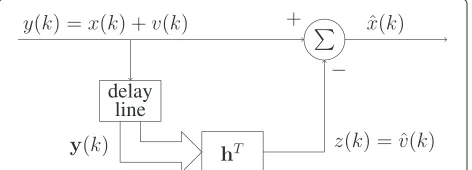
Secondly, we estimate the desired signal,x(k), as

x(k)=y(k)−v(k)=x(k)+v(k)−

An overview of the estimation process is shown in the block diagram in Figure 1.

Figure 1Block diagram of the estimation process.

Now, we find the βi’s that minimize the power of the residual noise, i.e., whereiLis the first column of theL×Lidentity matrix. We get

βi=iTLRvbi. (17)

Substituting (17) into (15), the estimator becomes

x(k)=x(k)+v(k)−

We deduce that the output SNR after noise reduction is

oSNRnr(hP)=

It is clear that the largerL−P is, the larger is the value of the output SNR. Also, from (18), we observe that the desired signal is not distorted so that the speech distortion index [1] is

The noise reduction factor [1] is

ξnr(hP)=

and since there is no signal distortion, we also have the relation:

oSNRnr(hP)

(4)

From (18), we find a class of distortionless estimators: y(k). The latter is the observation signal itself. It is obvious that the output SNR corresponding toxQ(k)is

4 Noise reduction filtering with distortion

In this section, we assume that the speech covariance matrix is full rank, i.e., equal to L. We can still use the method presented in the previous section, but this time we should expect distortion of the desired signal.

Again, we apply the filter:

h=h₀ h₁ · · · h_L₋₁T (27)

of lengthLto the observation signal vector. Then, the filter output and output SNR are, respectively,

z(k)=hTx(k)+hTv(k) (28) With this choice ofh, the output SNR becomes

oSNRf

This time, however, the output SNR cannot be equal to 0, but we can make it as small as we desire. The larger is the value of oSNRf

h_P

, the more the speech signal is distorted. If we can tolerate a small amount of distortion, then we can still considerz(k)as an estimate of the noise,

v(k)=z(k)=hT_Py(k).

In the second stage, we estimate the desired signal as

x(k)=y(k)−v(k)

By minimizing the power of the residual noise:

J_rn =E

Substituting (34) into (32), we obtain

x(k)=x(k)−

We deduce that the output SNR and speech distortion index are, respectively,

The smallerPis compared toL, the larger is the distor-tion. Further, the speech distortion index is independent of the input SNR, as is the gain in SNR. This can be observed by multiplying eitherRxin (5) orRv in (6) by a constant c, which leads to a corresponding change in the input SNR. Insertion of the resultingλi’s andbi’s in (37) and (38) will show that the output SNR is changed by the factor c and that the speech distortion index is independent ofc.

The output SNR and the speech distortion index are related as follows:

(5)

Figure 2Spectrum of the signal vector,x(k), and the corresponding filter,hP.

Interestingly, the exact same estimator is obtained by minimizing the power of the residual desired signal:

J_rd =E ⎧ ⎪ ⎨ ⎪ ⎩ ⎡ ⎣x(k)−

L

i=P+1

β_ibT_ix(k)

⎤ ⎦

2⎫_⎪

⎬ ⎪ ⎭

=σ_x2−2 L

i=P+1

β_iiT_LRxbi+ L

i=P+1 λiβi2.

(41)

Again, minimizingJ_rn orJ_rd leads to the estimatorx(k). Alternatively, another set of estimators can be obtained by minimizing the mean squared error betweenx(k)and

x(k):

J_mse =E ⎧ ⎪ ⎨ ⎪ ⎩ ⎡ ⎣v(k)−

L

i=P+1

β_ibT_iv(k)− L

i=P+1

β_ibT_i x(k)

⎤ ⎦

2⎫_⎪

⎬ ⎪ ⎭

=σ_v2−2 L

i=P+1

β_iiT_LRvbi+ L

i=P+1

(1+λi)βi2,

(42)

which leads to

β_i= i T LRvbi

1+λ_i. (43)

In the special case whereP=0, the estimator is the well-known Wiener filter.

5 Simulations

In this section, the filter design with and without tion is evaluated through simulations. Firstly, the distor-tionless case is considered in order to verify that the basics of the filter design hold and the filter works as expected. Secondly, we turn to the filter design with distortion to investigate the influence of the input SNR and the choice ofPon the output SNR and the speech distortion index.

The distortionless filter design was tested by the use of a synthetic harmonic signal. The use of such a signal makes it possible to control the rank of the signal covariance

(6)

Figure 4Performance as a function ofLfor a signal with rank-deficient covariance matrix.(a)Output SNR and(b)speech distortion index as a function of the filter length,L, for a real synthetic harmonic signal simulating voiced speech.

matrix, which is a very important feature in the present study. Further, the harmonic signal model is used to model voiced speech, e.g., in [24]. The harmonic signal model has the form:

x(k)= M

m=1

Amcos(m2πf0/fsk+φm) (44)

where Mis the model order,Am > 0 andφm ∈[ 0, 2π] are the amplitude and phase of themth harmonic,f0 ∈

[0,π/m] is the fundamental frequency, andfsis the

sam-pling frequency. The rank of the signal covariance matrix, Rx, is then P = 2M. In the simulations M = 5, the amplitudes are decreasing with the frequency, f, as 1/f, normalized to give A1 = 1, and the fundamental

fre-quency is chosen randomly such thatf0 ∈[ 150, 250] Hz,

the sampling frequency is 8 kHz, and the phases are ran-dom. The covariance matrices ofRxandRvare estimated from segments of 230 samples and are updated along with the filter for each sample. The number of samples is 1,000.

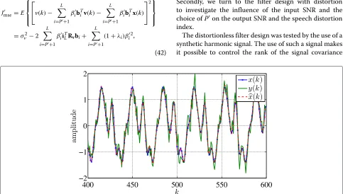
As an example, the spectrum of a synthetic signal is shown in Figure 2 along with the frequency response of the corresponding filter. The fundamental frequency is in this case f0 = 200 Hz, and the filter has a length

of L = 110. After subtraction of the filter output from the noisy observation, the estimate of the desired signal, shown in Figure 3, results. The desired signal and the noisy observation are shown as well. Comparing the sig-nals, it is easily seen that the filtering has improved the output SNR in the estimated signal relative to the noisy observation.

In order to support this, 100 Monte Carlo simulations have been performed for different lengths of the filter, and the performance is evaluated by the output SNR and speech distortion index. The output SNR is calcu-lated according to (10) as the ratio of the variances of the desired signal after noise reduction, [x(k)−hT_Px(k)], and the noise after noise reduction, [v(k)−hT_Pv(k)], whereas the speech distortion index is calculated according to (21) as the ratio of the variance of the filtered desired signal to the variance of the original desired signal. As seen in

a

b

(7)

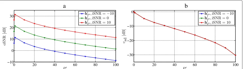
Figure 6Performance as a function ofP.(a)Output SNR and(b)speech distortion index as a function ofPfor a speech signal with full-rank covariance matrix.

Figure 4a, it is definitely possible to increase the SNR, but the extent is highly dependent on the length of the filter. For short filter lengths, the filter has almost no effect and oSNR≈iSNR, but as the filter length is increased, the out-put SNR is increased as well. Even though the estimates of the covariance matrices worsen when the filter length is increased, the longest filter gives rise to the best out-put SNR. By increasing the filter length from 20 to 110, a gain in SNR of more than 15 dB can be obtained. The cor-responding speech distortion index, shown in Figure 4b, is zero for all filter lengths, as was the basis for the filter design. As a reference, results for the Wiener filter (hw) are

shown as well. The Wiener filter is constructed based on [15] where it is derived based on joint diagonalization. The proposed method has a slightly lower output SNR, espe-cially at short filter lengths. On the other hand, the Wiener filter introduces distortion of the desired signal at all filter lengths, whereas the proposed filter is distortionless.

When the covariance matrix of the desired signal is full rank, speech distortion is introduced in the recon-structed speech signal. This situation was evaluated by

the use of autoregressive (AR) models, since these can be used to describe unvoiced speech [25]. The models used were of second order, and the coefficients were found based on ten segments of unvoiced speech from the Keele database [26], resampled to give a sampling frequency of 8 kHz and a length of 400 samples after resampling. Again,Pwas set to 10, the signal was added white Gaus-sian noise to give an average input SNR of 10 dB, and 100 Monte Carlo simulations were run on each of the ten generated signals in order to see the influence of the fil-ter length when the signal covariance matrix is full rank. The results are shown in Figure 5. As was the case for voiced speech, it is possible to gain approximately 15 dB in SNR by increasing the filter length from 20 to 110. How-ever, this time the speech distortion is also dependent on the filter length, and the longer the filter, the more signal distortion. In this case, comparison to the Wiener filter shows just the opposite situation than with the harmonic model. Now, the gain in SNR is higher for the proposed method for all filter lengths, but the signal is also more distorted.

(8)

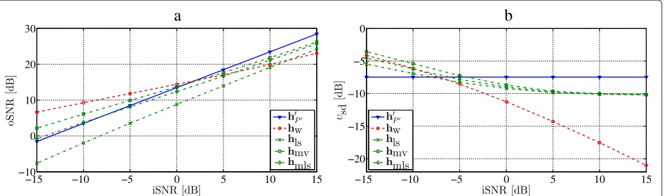
Figure 8Performance as a function of the input SNR.(a)Output SNR and(b)speech distortion index as a function of the input SNR for a speech signal with full-rank covariance matrix.

After having investigated the filter performance for dif-ferent filter lengths using synthetic signals, the influence of input SNR and the choice ofPare investigated directly in speech signals. Again, we used signals from the Keele database withfs=8 kHz. Excerpts with a length of 20,000

were extracted from different places in the speech signals from two male and two female speakers. Noise was added to give the desired average input SNR, and filters with a lengthL=110 and varyingPwere applied. Three differ-ent kinds of noise were used - white Gaussian, babble, and car noise - the last two from the AURORA database [27]. The output SNR and signal distortion index are depicted as a function ofPin Figure 6. Both the output SNR and the speech distortion index are decreasing withP, as was depicted in Section 4. Thereby, the choice ofP will be a compromise between a high output SNR and a low speech distortion index. In Figure 7, the proposed filter is com-pared, at an input SNR of 10 dB, to the Wiener filter, and three filters from [10] (hls,hmv,hmls), which are

subspace-based filters as well. These filters are subspace-based on a Hankel

representation of the observed signal, which we, from the segment length of 230 samples, construct with a size of 151×80. Due to restrictions on the chosen rank (accord-ing toP), this is only varied from 1 to 71. The performance of the Wiener filter is of course independent of P, and it is, therefore, possible to construct a filter that either gives a higher output SNR or a lower speech distortion than the Wiener filter, dependent on the choice ofP. The filters from [10] are dependent onPas well, but the pro-posed filter has a broader range of possible combinations of output SNR and speech distortion. AtP=1, a gain in output SNR of approximately 5 dB can be obtained while the speech distortion is comparable. At the other extreme, it is possible to obtain the same output SNR ashlswhile

the speech distortion index is lowered by approximately 5 dB.

The choice of the value of P is, however, not depen-dent on the input SNR, as seen in Figure 8, since both the gain in SNR and the speech distortion index are constant functions of the input SNR, as was also found theoretically

(9)

Table 1 PESQ scores at different filter lengths and SNRs for

P=31

SNR [dB] hP,P

₌₃₁

L=70 L=90 L=110

0 2.160 2.353 2.467

5 2.476 2.656 2.737

10 2.808 2.919 2.920

in Section 4. This means that it is possible to construct a filter according to the desired combination of gain in SNR and speech distortion, and then this will apply no matter the input SNR. This is not the case for either the Wiener filter or the filters from [10] as seen in Figure 9. For these filters, the gain in SNR is decreasing with input SNR (except forhlswhich is also constant) as is the speech

distortion index.

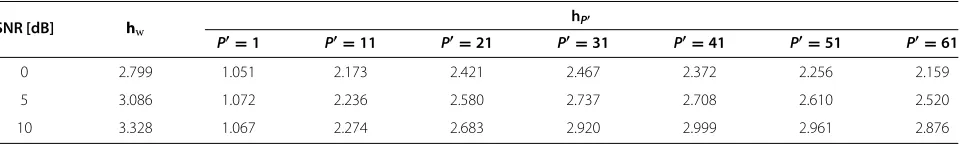
As a measure of the subjective evaluation, Perceptual Evaluation of Speech Quality (PESQ) scores [28] have been calculated for different filter lengths, different values ofP, and different SNRs. The used speech signal contains 40,000 samples from the beginning of the speech signal from the first female speaker in the Keele database. The results are shown in Tables 1 and 2. It is seen that the PESQ scores are increasing with increasing filter length and SNR, even though the effect of going from a filter length of 90 to 110 seems smaller than increasing the length from 70 to 90. The PESQ score is rather low for low values ofP, peaks forP= 31 orP=41, depending on the SNR, and then decreases again for higher val-ues of P. This is also heard in informal listening tests of the resulting speech signal. At low values of P, the speech signal sounds rather distorted, whereas at high levels of P, the signal is noisy, but not very distorted, which also confirms the findings in Figure 6. As reflected in the PESQ score, a signal with a compromise between the two is preferred if the purpose is listening directly to the output. In such a context, the performance of the Wiener filter is slightly better than the proposed filter with PESQ scores approximately 0.3 units larger. However, the purpose of noise reduction is sometimes as a pre-processor to, e.g., a speech recognition algorithm. Here, the word error rate increases when the SNR decreases [29,30], but on the other hand, the algorithms are also

sensible to distortion of the speech signal [31,32]. In such cases, it might, therefore, be optimal with another rela-tionship between SNR and speech distortion than the one having the best perceptual performance. This opti-mization is possible with the proposed filter due to its flexibility.

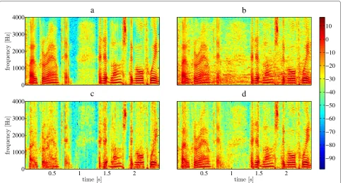
The effect of choosing different values ofP is visual-ized in Figure 10. Figure 10a shows the spectrogram of a piece of a clean speech signal from the Keele database, and in Figure 10b, babble noise was added to give an average input SNR of 10 dB. Figure 10c,d shows the spec-trograms of the reconstructed speech signal with two different choices of P. The former is a reconstruction based onP=10. Definitely, the noise content is reduced when comparing to the noisy speech signal in Figure 10b. However, a high degree of signal distortion has been intro-duced as well, which can be seen especially in the voiced speech parts, where the distinction between the harmon-ics is blurred compared to both the clean speech signal and the noisy speech signal. In the latter figure,P = 70, and therefore, both noise reduction and signal distortion are not as prominent as when P = 10. Here, the har-monics are much more well preserved, but, as is seen in the background, it comes with the price of less noise reduction.

A feature of the proposed filter, which is not explored here, is the possibility of choosing different values ofP over time. The optimal value ofP depends on whether the speech is voiced or unvoiced, and how many harmon-ics there are in the voiced parts. By adapting the value of Pat each time step based on this information, it should be possible to simultaneously achieve a higher SNR and a lower distortion.

6 Conclusions

In this paper, we have presented a new perspective on time-domain single-channel noise reduction based on forming filters from the eigenvectors that diagonalize both the desired and noise signal covariance matrices. These filters are chosen so that they provide an estimate of the noise signal when applied to the observed signal. Then, by subtraction of the noise estimate from the observed signal, an estimate of the desired signal can be obtained. Two cases have been considered, namely one where no

Table 2 PESQ scores for different values ofPand SNR for a filter length of 110

SNR [dB] hw

hP

P₌1 P₌11 P₌21 P₌31 P₌41 P₌51 P₌61

0 2.799 1.051 2.173 2.421 2.467 2.372 2.256 2.159

5 3.086 1.072 2.236 2.580 2.737 2.708 2.610 2.520

(10)

a

b

c

d

Figure 10Spectra of desired signal, noisy signal and two reconstructions with different choices ofP.(a)Spectrum of a part of a speech signal from the Keele database.(b)Speech signal from (a) contaminated with babble noise to give an average input SNR of 10 dB.(c)Reconstructed speech signal usingP=10.(d)Reconstructed speech signal usingP=70.

distortion is allowed on the desired signal and one where distortion is allowed. The former case applies to signals that have a rank that can be assumed to be less than the rank of the observed signal covariance matrix, which is, for example, the case for voiced speech. The latter case applies to desired signals that have a full-rank covari-ance matrix. In this case, the only way to achieve noise reduction is by also allowing for distortion on the desired signal. The amount of distortion introduced depends on a parameter corresponding to the rank of an implicit approximation of the desired signal covariance matrix. As such, it is relatively easy to control the trade-off between noise reduction and speech distortion. Experiments on real and synthetic signals have confirmed these principles and demonstrated how it is, in fact, possible to achieve higher output signal-to-noise ratio or a lower signal dis-tortion index with the proposed method than with the classical Wiener filter. Moreover, the results show that only a small loss in output signal-to-noise ratio is incurred when no distortion can be accepted, as long as the filter is not too short. The results also show that when distortion is allowed on the desired signal, the amount of distor-tion is independent of the input signal-to-noise ratio. The presented perspective is promising in that it unifies the ideas behind subspace methods and optimal filtering, two methodologies that have traditionally been seen as quite different.

Competing interests

The authors declare that they have no competing interests.

Acknowledgements

This research was supported by the Villum Foundation and the Danish Council for Independent Research, grant ID: DFF - 1337-00084.

Author details

1_{Audio Analysis Lab, Department of Architecture, Design and Media}

Technology, Aalborg University, Aalborg 9220, Denmark.2_{INRS-EMT, University}

of Quebec, Montreal, QC H2X 1L7, Canada.

Received: 19 December 2013 Accepted: 17 March 2014 Published: 26 March 2014

References

1. J Benesty, J Chen,Optimal Time-Domain Noise Reduction Filters – A Theoretical Studyvol. VII, 1st edn. (Springer, Heidelberg, 2011)

2. S Boll, Suppression of acoustic noise in speech using spectral subtraction. IEEE Trans. Acoust., Speech, Signal Process.27(2), 113–120 (1979) 3. RJ McAulay, ML Malpass, Speech enhancement using a soft-decision

noise suppression filter. IEEE Trans. Acoust., Speech, Signal Process.

28(2), 137–145 (1980)

4. Y Ephraim, D Malah, Speech enhancement using a minimum mean-square error log-spectral amplitude estimator. IEEE Trans. Acoust., Speech, Signal Process.33(2), 443–445 (1985)

5. S Srinivasan, J Samuelsson, WB Kleijn, Codebook-based Bayesian speech enhancement for nonstationary environments. IEEE Trans. Audio, Speech, and Language Process.15(2), 441–452 (2007)

6. Y Ephraim, HL Van Trees, A signal subspace approach for speech enhancement. IEEE Trans. Speech Audio Process.3(4), 251–266 (1995) 7. SH Jensen, PC Hansen, SD Hansen, JA Sørensen, Reduction of broad-band

noise in speech by truncated QSVD. IEEE Trans. Speech Audio Process.

(11)

8. J Benesty, J Chen, Y Huang, I Cohen,Noise Reduction in Speech Processing

(Springer, Heidelberg, 2009)

9. P Loizou,Speech Enhancement: Theory and Practice(CRC Press, Boca Raton, 2007)

10. PC Hansen, SH Jensen, Subspace-based noise reduction for speech signals via diagonal and triangular matrix decompositions: survey and analysis. EURASIP J. Adv. Signal Process.2007(1), 24 (2007)

11. S Rangachari, P Loizou, A noise estimation algorithm for highly nonstationary environments. Speech Commun.28, 220–231 (2006) 12. I Cohen, Noise spectrum estimation in adverse environments: improved

minima controlled recursive averaging. IEEE Trans. Speech Audio Process.

11(5), 466–475 (2003)

13. T Gerkmann, RC Hendriks, Unbiased MMSE-based noise power estimation with low complexity and low tracking delay. IEEE Trans. Audio, Speech, Lang. Process.20(4), 1383–1393 (2012)

14. RC Hendriks, R Heusdens, J Jensen, U Kjems, Low complexity DFT-domain noise PSD tracking using high-resolution periodograms. EURASIP J. Appl. Signal Process.2009(1), 15 (2009)

15. S Doclo, M Moonen, GSVD-based optimal filtering for single and multimicrophone speech enhancement. IEEE Trans. Signal Process.

50(9), 2230–2244 (2002)

16. M Souden, J Benesty, S Affes, On optimal frequency-domain multichannel linear filtering for noise reduction. IEEE Trans. Audio, Speech, Lang. Process.18(2), 260–276 (2010)

17. J Benesty, M Souden, J Chen, A perspective on multichannel noise reduction in the time domain. Appl. Acoustics.74(3), 343–355 (2013) 18. RC Hendriks, T Gerkmann, Noise correlation matrix estimation for

multi-microphone speech enhancement. IEEE Trans. Audio, Speech, Lang. Process.20(1), 223–233 (2012)

19. MG Christensen, A Jakobsson, Optimal filter designs for separating and enhancing periodic signals. IEEE Trans. Signal Process.58(12), 5969–5983 (2010)

20. JR Jensen, J Benesty, MG Christensen, SH Jensen, Enhancement of single-channel periodic signals in the time-domain. IEEE Trans. Audio, Speech, Lang. Process.20(7), 1948–1963 (2012)

21. JR Jensen, J Benesty, MG Christensen, SH Jensen, Non-causal

time-domain filters for single-channel noise reduction. IEEE Trans. Audio, Speech, Lang. Process.20(5), 1526–1541 (2012)

22. LJ Griffiths, CW Jim, An alternative approach to linearly constrained adaptive beamforming. IEEE Trans. Antennas Propag.30(1), 27–34 (1982) 23. JN Franklin,Matrix Theory(Prentice-Hall, New York, 1968)

24. J Jensen, JHL Hansen, Speech enhancement using a constrained iterative sinusoidal model. IEEE Trans. Speech Audio Process.9(7), 731–740 (2001) 25. JR Deller, JHL Hansen, JG Proakis,Discrete-Time Processing of Speech

Signals(Wiley, New York, 2000)

26. F Plante, GF Meyer, WA Ainsworth, A pitch extraction reference database, inProc. Eurospeech(Madrid, Spain, 18–21 September 1995), pp. 837–840 27. D Pearce, HG Hirsch, The AURORA experimental framework for the

performance evaluation of speech recognition systems under noisy conditions, inProc. Int. Conf. Spoken Language Process(Beijing, China, 16–20 October 2000), pp. 29–32

28. Y Hu, P Loizou, Evaluation of objective quality measures for speech enhancement. IEEE Trans. Speech Audio Process.16(1), 229–238 (2008) 29. X Cui, A Alwan, Noise robust speech recognition using feature

compensation based on polynomial regression of utterance SNR. IEEE Trans. Speech Audio Process.13(6), 1161–1172 (2005)

30. RP Lippmann, Speech recognition by machines and humans. Speech Commun.22(1), 1–15 (1997)

31. JM Huerta, RM Stern, Distortion-class weighted acoustic modeling for robust speech recognition under GSM RPE-LTP coding, inProc. of the Robust Methods for Speech Recognition in Adverse Conditions(Tampere, Finland, 25–26 May 1999), pp. 11–14

32. T Takiguchi, Y Ariki, PCA-based speech enhancement for distorted speech recognition. J. Multimedia.2(5), 13–18 (2007)

doi:10.1186/1687-6180-2014-37

Cite this article as:Nørholmet al.:Single-channel noise reduction using unified joint diagonalization and optimal filtering. EURASIP Journal on Advances in Signal Processing20142014:37.

Submit your manuscript to a

journal and beneﬁ t from:

7Convenient online submission 7Rigorous peer review

7Immediate publication on acceptance 7Open access: articles freely available online 7High visibility within the ﬁ eld

7Retaining the copyright to your article