Open Access
Proceedings
Application of an iterative Bayesian variable selection method in a
genome-wide association study of rheumatoid arthritis
Soonil Kwon, Dai Wang and Xiuqing Guo*
Address: Medical Genetics Institute, Cedars-Sinai Medical Center, 8635 West Third Street, Suite 665, Los Angeles, California 90048, USA
Email: Soonil Kwon - [email protected]; Dai Wang - [email protected]; Xiuqing Guo* - [email protected] * Corresponding author
Abstract
Genome-wide association studies usually involve several hundred thousand of single-nucleotide polymorphisms (SNPs). Conventional approaches face challenges when there are enormous number of SNPs but a relatively small number of samples and, in some cases, are not feasible. We introduce here an iterative Bayesian variable selection method that provides a unique tool for association studies with a large number of SNPs (p) but a relatively small sample size (n). We applied this method to the simulated case-control sample provided by the Genetic Analysis Workshop 15 and compared its performance with stepwise variable selection method. We demonstrated that the results of iterative Bayesian variable selection applied to when p » n are as comparable as those of stepwise variable selection implemented to when n » p. When n > p, the iterative Bayesian variable selection performs better than stepwise variable selection does.
Background
Advances in genotyping technology have made genome-wide association studies feasible. Usually, a large number of single-nucleotide polymorphisms (SNPs) are engaged in a genome-wide association study. Many statistical approaches have been used to analyze the genome-wide association data. Conventional statistical approaches, however, face many challenges for analyzing the data in which a relatively small number of samples that are real-istic to recruit for a research study contain hundreds of thousands of markers densely spaced over the genome. Various statistical approaches that can be utilized when p » n have been applied to reduce dimension. West et al. [1] utilized singular value decomposition in the design
matri-ces of Bayesian regression analysis with binary responses. Sha et al. [2] applied stochastic search variable selection, which is a Bayesian variable selection (BVS) approach proposed by George and McCulloch [3], to identify molecular signatures of disease stage.
Although shown to be very promising, BVS uses quite long iterations and take a long time to search for signifi-cant SNPs. In order to overcome these problems, we pro-pose an iterative Bayesian variable selection (IBVS) method, which repeatedly uses the BVS with relatively small iterations until a proper number of SNPs are selected. We applied the IBVS to randomly selected sub-samples of the simulated rheumatoid arthritis (RA) data
from Genetic Analysis Workshop 15
St. Pete Beach, Florida, USA. 11–15 November 2006
Published: 18 December 2007
BMC Proceedings 2007, 1(Suppl 1):S109
<supplement> <title> <p>Genetic Analysis Workshop 15: Gene Expression Analysis and Approaches to Detecting Multiple Functional Loci</p> </title> <editor>Heather J Cordell, Mariza de Andrade, Marie-Claude Babron, Christopher W Bartlett, Joseph Beyene, Heike Bickeböller, Robert Culverhouse, Adrienne Cupples, E Warwick Daw, Josée Dupuis, Catherine T Falk, Saurabh Ghosh, Katrina A Goddard, Ellen L Goode, Elizabeth R Hauser, Lisa J Martin, Maria Martinez, Kari E North, Nancy L Saccone, Silke Schmidt, William Tapper, Duncan Thomas, David Tritchler, Veronica J Vieland, Ellen M Wijsman, Marsha A Wilcox, John S Witte, Qiong Yang, Andreas Ziegler, Laura Almasy and Jean W MacCluer</editor> <note>Proceedings</note> <url>http://www.biomedcentral.com/content/pdf/1753-6561-1-S1-info.pdf</url> </supplement>
This article is available from: http://www.biomedcentral.com/1753-6561/1/S1/S109
© 2007 Kwon et al; licensee BioMed Central Ltd.
provided by the Genetic Analysis Workshop 15 (GAW15) Problem 3 to find subsets of SNPs that are associated with RA status. The results obtained by using IBVS were com-pared to those obtained from stepwise variable selection (SVS) to evaluate the validity and performance of IBVS.
Methods
Bayesian variable selection with probit model
The binary probit model is incorporated to implement BVS method. Let us assume that (y, X) indicates the observed data, with yn × 1 a dichotomous categorical out-come vector coded as 1 or 0 representing for RA affected or RA unaffected, respectively, and Xn × p the predictor matrix. Let z be an n × 1 vector of latent variables, while each zi, associated with a categorical outcome, yi, is described by a linear regression model:
zi = Xiβ+ εi, ε~ N(0, σ2), i = 1,..., n.
The relationship between zi and yi is defined by yi = 1 if zi > 0 and yi = 0 otherwise. The likelihood function of the model defined in Eq. (1) may be written as f(z|β, σ):
f(z|β, σ) = Nn(Xβ, σ2I).
The variable selection problem arises from the fact that it would be preferable to exclude some unknown subset of the predictors that have negligible influence on the out-come. Thus, statistical models for the variable selection problem can be represented by a selection vector, which is a set of binary indicator variables γ= (γ1,..., γp), where γj = 1 or 0 corresponds to inclusion or exclusion of predictor j in the model, respectively. The prior distribution of the model indicator variables, π(γ), is chosen to reflect prior belief in whether particular SNPs are associated with RA status in our case. A reasonable choice of the prior infor-mation might be to have the γj (j = 1,..., p) independent with probability π(γj = 1) = 1-π(γj = 0) = pj, thus
π(γ) = ∏ pjγj (1-pj)1-γj.
The residual variance σ2 for the γth model is modeled as a
realization from an inverse gamma prior:
π(σ2|γ) = IG(ν/2, νλγ)
which is equivalent to νλγ ~ χν2. Because the value of selec-tion vector, γ, is of interest and is unknown, the uncer-tainty underlying variable selection can be modeled by a mixture prior:
π(β, σ, γ) = π(β|σ, γ) π(σ|γ) π(γ).
The posterior distribution of (β, σ, γ) can be obtained from the product of the likelihood function of the model in Eq. (2) and the prior defined in Eq. (5):
π(β, σ, γ|z) = f(z|β, σ) π(β|σ, γ) π(σ|γ) π(γ).
Therefore, integrating out βand σfrom Eq. (6) yields the posterior distribution of the selection vector γ:
π(γ|z) ≈ g(γ) ≡ π(γ) ∫ f(z|β, σ) π(β|σ, γ) π(σ|γ) π(γ) dβdσ.
Based on this setting, Metropolis algorithm with Gibbs sampling was incorporated to sample (γ, z) as follows: 1) Metropolis step: π(γ|z) ≈ g(γ) with acceptance probability {g(γnew)/g(γold), 1}; 2) (z|γ, X) has a truncated normal
dis-tribution.
In order to update each transition from γold to γnew, the
Metropolis algorithm uses deletion, addition, and swap-ping moves discussed by Brown et al. [4]. Details of the prior information, the posterior distribution, and the updating procedure can be found in George and McCul-loch [5] and Sha et al. [2].
Iterative Bayesian variable selection
As mentioned, BVS uses long iterations and take a long time for the Metropolis algorithm to find suitable subset of SNPs. In the worst case, BVS might be unable to provide a promising subset. In order to overcome these problems, we propose to use BVS iteratively with a relatively small number of iterations, which is termed IBVS, to increase the speed of search for promising subsets of SNPs. There are two basic ideas behind IBVS. First, if γj is not significant at the early stage of iteration when long iteration is incor-porated in BVS, then the jth marker is excluded in the final
model. Second, the model that has high probability is more likely to appear at the early stage of iteration. From these facts, we can use BVS iteratively with relatively small number of iterations to increase the speed of searching for promising subsets of markers. This IBVS can be imple-mented by the following steps: 1) Start with BVS with full model, i.e., the model having all SNPs. 2) Choose a model for next iteration of BVS, e.g., the model that has highest posterior probability. 3) Repeat Step 1 and 2 with the model chosen in Step 2 until a certain number of SNPs remain in the model.
Materials
inter-marker distance of about 5 cM; 2) a set of 9187 SNPs dis-tributed on the genome to mimic a 10 K SNP chip set; 3) a very dense map of 17,820 SNPs on chromosome 6. We utilized the second marker set for our analysis. According to the answer distributed by GAW15, there are three loci (DR, C, and D) on chromosome 6 that increase the risk of RA. Loci DR and C are located between SNP6_153 and SNP6_154, and are in complete linkage equilibrium. Locus C increases RA risk only in women. Locus D is located between SNP6_161 and SNP6_162, and has a rare minor allele frequency of 0.0083. We focused our analysis on the 674 SNPs on chromosome 6 to evaluate the IBVS method.
We first constructed three case-control panels for each of the 100 replicates. The first panel included both males and females. One affected offspring was randomly selected from each of the 1500 families that had an ASP. These 1500 unrelated affected subjects were used as cases. The 2000 unrelated control subjects were used as controls. In addition, because locus C increases RA risk only in women, we also constructed a female case-control panel and a male case-control panel. To maximize the number of female cases, we randomly selected one affected female offspring from each of the ASP families that had at least one female offspring. The female case-control panel con-sisted of ~1400 unrelated affected female offspring selected from the ASP families and ~1000 female controls. The male case-control panel was constructed similarly. It consisted of ~680 cases and ~1000 controls. Therefore, a total of three case-control panels (total, female, and male, respectively), each having 100 replicates, were con-structed. This data set was named DS1.
Second, in order to evaluate the performance of IBVS when p » n, we constructed a subset case-control panel from each of the case-control panels in DS1 by randomly selecting 50 cases and 50 controls. The same 674 SNPs
were kept in the panel. This data set was called DS2 (n = 100, p = 674).
Finally, in order to compare the performance between IBVS and traditional SVS directly, we selected a subset of 50 SNPs located between SNP6_128 and SNP6_177 from DS2. This dataset was named DS3 (n = 100, p = 50).
As a comparison, we also carried out the association anal-ysis using BVS and SVS, which was implemented in the Proc Logistic procedure in SAS. We summarized all results obtained from IBVS, BVS, and SVS by calculating power for each SNP indicator, γj, as follows:
where I is the indicator function satisfying I(γij = 1) = 1 if
γij = 1 and I(γij = 1) = 0 otherwise; and n is the total number of replicates. Like other iterative methods, e.g., Newton method, there can be many stopping rules that can be applied in Step 3 in IBVS. We used the predetermined number of SNPs (10) based on empirical experience to stop the IBVS algorithm.
Results and discussion
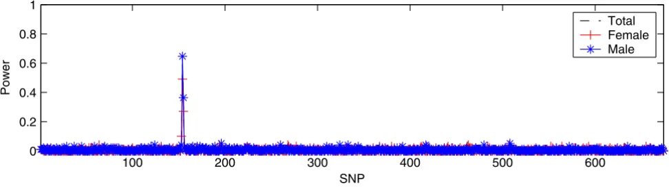
We examined the performance of IBVS when p » n by implementing the IBVS in DS2 and summarized the results in Figure 1. We found a peak corresponding to the genomic region where loci DR and C are located for all three panels (total, female, and male), demonstrating that IBVS properly identified two trait loci (DR and C). Figure 1 also shows that IBVS was unable to identify locus D. This is, however, not completely unexpected due to the fact that the minor allele frequency in locus D is very low (0.0083), and we have more predictors (674 SNPs) than samples (100).
IBVS in DS2. All three panels in DS2 have 100 samples (50 cases and 50 controls) and 674 SNPs. 1
100 200 300 400 500 600
Figure 2 shows the results when applying SVS to DS1. For all three panels, SVS successfully identified three trait loci (DR, C, and D) with two high peaks. One peak corre-sponded to the region between SNP6_153 and SNP6_154, where loci DR and C are located, and the other corresponded to SNP6_162, where locus D is located. However, there were a few other SNPs with relatively high powers around SNP6_145, but those were apparently false positives.
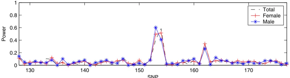
Although we illustrated the validity of IBVS by comparing the results obtained from SVS, it was difficult to directly compare two search methods given that they were applied to two different data sets (100 samples of DS1 and ~3500 samples of DS2). In order to compare the performance between IBVS and SVS directly, we applied both methods to DS3, which focused on the SNPs between SNP6_128 and SNP6_177 (n = 100, p = 50). The results obtained from IBVS and SVS are shown in Figure 3 and Figure 4, respectively. Figure 3 shows that, for each of the three
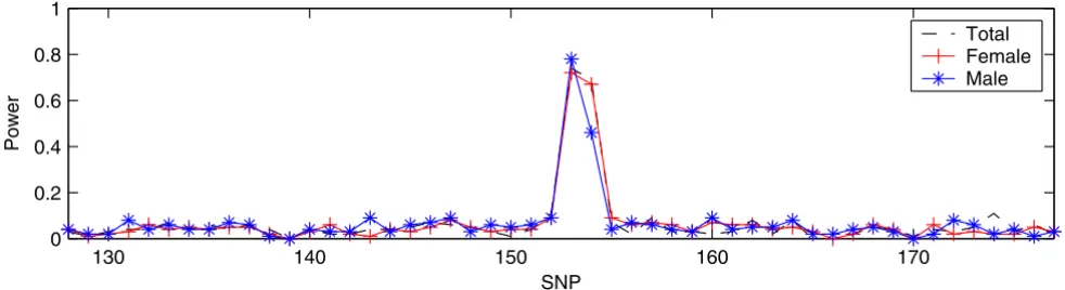
case-control panels, there are two separated peaks: one relatively high peak at SNP6_153 and SNP6_154 and the other at SNP6_162. This demonstrated that IBVS success-fully identified three trait loci (DR, C, and D) including the one with a rare allele frequency. However, the results from SVS had only one peak corresponding to loci DR and C for all the three case-control panels (Figure 4). SVS was unable to identify locus D, which has a very small minor allele frequency. Therefore, we concluded that the per-formance of IBVS is better than that of SVS when n > p.
We also applied BVS to DS2 to compare the performance between IBVS and BVS. The results showed that the final model provided by BVS with 10,000 iterations and 5000 burn-in periods for each replicate contained over 300 SNPs, which demonstrated that BVS tends to yield more false positives. Therefore, IBVS improved the performance in variable selection as compared to BVS. In addition, the overall run time for BVS was about five times slower than that for IBVS.
IBVS in DS3
Figure 3
IBVS in DS3. All three panels in DS3 have 100 samples (50 cases and 50 controls) and 50 SNPs. 1
130 140 150 160 170
0 0.2 0.4 0.6 0.8
Total Female Male
SNP
Power
SVS in DS1
Figure 2
SVS in DS1. Total panel has 1500 cases and 2000 controls; female panel, ~1400 cases and ~1000 controls; and male panel, ~680 cases and ~1000 controls. All panels have 674 SNPs.
1
100 200 300 400 500 600
0 0.2 0.4 0.6 0.8
Total Female Male
SNP
With the goal of investigating sample size effect in IBVS, we applied IBVS to a data set, in which each case-control panel had five cases and five controls randomly selected from each case-control panel in DS1 and 50 SNPs between SNP6_128 and SNP6_177 (n = 10, p = 50). We found that IBVS identified the same two loci (DR and C), as when applied to DS2 (Figure 1), but was unable to identify Locus D, although the power was lower than that in Figure 1.
Another interesting question is how SNP density affects the performance of IBVS. We applied IBVS to another data set in which each case-control panel again consists of ten cases and controls (five each) randomly selected from each of case-control panels in DS1, but the 50 SNPs were selected in a wide genomic region (between SNP6_104 and SNP6_203) by selecting every other SNP. With this data set, we were able to identify SNP6_154 with a slightly higher power as compared to that with a denser SNP map. The likely reason for this is that the between-variable cor-relation included in the model has an effect on the per-formance of the method. When the SNPs are relatively loosely distributed, the LD (between-variable correlation) among them is lower and IBVS performs better. However, this does not mean we will be able to identify a disease mutation with very loosely distributed SNPs. The success of a genome-wide association study still relies on whether a marker in high LD with the disease mutation is included in the study set of SNPs.
Conclusion
We applied the IBVS method to the case-control data con-structed from the simulated RA data sets of GAW15. When the number of sample size (100 observations) is larger than the number of predictors (50 SNPs), i.e., n > p, we were able to identify association with RA status on chro-mosome 6 at the location where loci DR and C are located by both IBVS and SVS. However, the association between
RA status and locus D was identified only by IBVS. With a small sample size of 100 and large number of predictors (674 SNPs), i.e., n » p, IBVS can still identify association with RA status on chromosome 6 at the location of Loci DR and C. We concluded that IBVS method is promising for identifying genetic determinants in genome-wide association studies when the number of genetic markers is much larger than the number of samples.
Competing interests
The author(s) declare that they have no competing inter-ests.
Acknowledgements
This article has been published as part of BMC Proceedings Volume 1 Sup-plement 1, 2007: Genetic Analysis Workshop 15: Gene Expression Analysis and Approaches to Detecting Multiple Functional Loci. The full contents of the supplement are available online at http://www.biomedcentral.com/ 1753-6561/1?issue=S1.
References
1. West M, Nevins JR, Marks JR, Spang R, Zuzan H: DNA microarray data analysis and regression modeling for genetic expression profiling. Discussion Paper 00-15 2000 [http://ftp.stat.duke.edu/ WorkingPapers/00-15.html]. Durham, NC: Institute of Statistics and Decision Science, Duke University
2. Sha N, Vannucci M, Tadesse M, Brown P, Dragoni I, Davies N, Rob-erts T, Contestabile A, Salmon M, Buckley C, Falciani F: Bayesian variable selection in multinomial probit models to identify molecular signatures of disease stage. Biometrics 2004,
60:812-819.
3. George E, McCulloch R: Variable selection via Gibbs sampling.
J Am Stat Assoc 1993, 88:881-889.
4. Brown P, Vannucci M, Fearn T: Multivariate Bayesian variable selection and prediction. J Roy Stat Soc Series B 1998, 60:627-641. 5. George E, McCulloch R: Approaches for Bayesian variable
selection. Stat Sinica 1997, 7:339-373. SVS in DS3
Figure 4
SVS in DS3. All three panels in DS3 have 100 samples (50 cases and 50 controls) and 50 SNPs. 1
130 140 150 160 170
0 0.2 0.4 0.6 0.8
Total Female Male
SNP