R E S E A R C H
Open Access
On the performance of parallelisation
schemes for particle filtering
Dan Crisan
1, Joaquín Míguez
2,3*and Gonzalo Ríos-Muñoz
2,3Abstract
Considerable effort has been recently devoted to the design of schemes for the parallel implementation of sequential Monte Carlo (SMC) methods for dynamical systems, also widely known as particle filters (PFs). In this paper, we present a brief survey of recent techniques, with an emphasis on the availability of analytical results regarding their performance. Most parallelisation methods can be interpreted as running an ensemble of lower-cost PFs, and the differences between schemes depend on the degree of interaction among the members of the ensemble. We also provide some insights on the use of the simplest scheme for the parallelisation of SMC methods, which consists in splitting the computational budget intoMnon-interacting PFs withNparticles each and then obtaining the desired estimators by averaging over theMindependent outcomes of the filters. This approach minimises the parallelisation overhead yet still displays desirable theoretical properties. We analyse the mean square error (MSE) of estimators of moments of the optimal filtering distribution and show the effect of the parallelisation scheme on the approximation error rates. Following these results, we propose a time–error index to compare schemes with different degrees of parallelisation. Finally, we provide two numerical examples involving stochastic versions of the Lorenz 63 and Lorenz 96 systems. In both cases, we show that the ensemble of non-interacting PFs can attain the approximation accuracy of a centralised PF (with the sametotalnumber of particles) in just a fraction of its running time using a standard multicore computer.
Keywords: Particle filtering, Parallelisation, Convergence analysis, Particle islands, Lorenz 63, Lorenz 96
1 Introduction
Over the past decade, there has been a continued interest in the design of schemes for the implementation of parti-cle filtering algorithms using parallel or distributed hard-ware of various types, including general purpose devices such as multi-core CPUs or graphical processing units (GPUs) [1] and application-tailored devices such as field-programmable gate arrays (FPGAs) [2]. A particle filter (PF) is a recursive algorithm for the approximation of the sequence of posterior probability distributions that arise from a stochastic dynamical system in state-space form (see, e.g. [3–6] and references therein for a general view of the field). A typical PF includes three steps that are repeated sequentially:
*Correspondence:[email protected]
2Department of Signal Theory and Communications, Universidad Carlos III de Madrid, Madrid, Spain
3Instituto de Investigación Sanitaria Gregorio Marañón (IiSGM), Madrid, Spain Full list of author information is available at the end of the article
• Monte Carlo sampling in the space of the state variables,
• Computation of weights for the generated samples and, finally,
• Resampling according to the weights.
While at first sight the algorithm may look straightfor-ward to parallelise (sampling and weighting can be carried out concurrently without any constraint), the resampling step involves the interaction of the whole set of Monte Carlo samples. Several authors have proposed schemes for ‘splitting’ the resampling step into simpler tasks that can be carried out concurrently. The approaches are diverse and range from the heuristic [7–9] to the mathemat-ically well-principled [2, 10–14]. However, the former are largely based on (often loose) approximations that prevent the claim of any rigorous guarantees of conver-gence, whereas the latter involve non-negligible overhead to ensure the proper interaction of particles.
The goal of this paper is to provide
(i) A survey of recently proposed, and mathematically well grounded, parallelisation schemes for particle filtering and
(ii) Analytical insights into the performance of the simplest parallelisation method, namely the averaging of statistically independent PFs.
Besides describing the various methodologies, we aim at characterising their performance analytically when-ever possible. For that purpose, we need to introduce accurate notation, unfortunately a bit more involved than needed for the mere description of the algorithmic steps. Then, we describe and provide a basic conver-gence result for the standard PF and proceed to describe four different approaches to its parallelisation: the sim-ple averaging of statistically independent (i.e. non inter-acting) low-complexity PFs, the method based on the distributed resampling with non-proportional allocation (DRNA) procedure of [2,10,11], the particle island model of [13, 14] and the adaptive interaction scheme termed α-sequential Monte Carlo (α-SMC) in [12].
The simplest parallelisation scheme consists in run-ning M statistically independent PFs with N particles (i.e. Monte Carlo samples) each and then averaging the M independent estimators. This approach has the lim-itation that the bias of the averaged estimator depends only on N. Hence, if N is relatively small, the bias is large even if we use a very high numberMof parallel fil-ters. This drawback can be overcome by allowing some degree of interaction among theMconcurrently running PFs. The DRNA, particle island andα-SMC approaches introduce this interaction in different flavours. In DRNA-based ensembles of PFs, each filter runs separately but it periodically exchanges a few particles with other mem-bers of the ensemble using a communication network [10]. Algorithms in the particle island class rely on two levels of resampling: conventional resampling at particle level and island-level resampling, where complete sets of particles (associated to parallel-running PFs) are repli-cated or eliminated stochastically [13, 14]. Finally, the α-SMC scheme of [12] is a very flexible methodology that enables the adaptive selection of different interaction pat-terns (i.e. which particles are resampled together) over time. For each one of these techniques, we describe the methodology and establish basic theoretical guarantees for convergence.
In the second part of the paper, we focus on the anal-ysis of the performance of the simplest parallelisation scheme, the averaging ofMstatistically independent PFs withNparticles each. Under mild assumptions, we anal-yse the mean square error (MSE) of the estimators of one-dimensional statistics of the optimal filtering distri-bution and show explicitly the effect of the parallelisation scheme on the convergence rate. Specifically, we study the
decomposition of the MSE into variance and bias compo-nents, to show that the variance isOMN1 , i.e. it decreases linearly with the total number of particles, while the bias is ON12
, i.e. it goes to 0 quadratically with N. These results have already been obtained, e.g. in [13] using the Feynman-Kac framework of [4]. Here, we aim at providing a self-contained analysis that illustrates the key theoreti-cal issues in the convergence of parallel PFs. All proofs are constructed from elementary principles, and we obtain explicit error rates (for the bias, the variance and the MSE) that hold for allMandN, while the theorems in [13] are strictly asymptotic. While we have focused here on PFs for discrete-time state-space models, the analysis can be similarly done for continuous-time systems, and, indeed, the basic results needed for that case can be found in [15]. Finally, in order to compare different parallelisation schemes, we introduce a time–error index that combines time complexity (asymptotic order of the running time) and estimation accuracy (asymptotic error rates) into a single quantitative figure of merit that can be used to compare schemes with different degrees of interaction.
The rest of the paper is organised as follows. In Section 2, we present basic background material, and notation, for the analysis of PFs. Section3is devoted to a survey of parallelisation schemes for particle filtering. Our analysis of the ensemble of non-interacting PFs is pre-sented in Section4. In Section5, we present numerical results for two examples, namely the filtering of stochastic versions of the Lorenz 63 and Lorenz 96 systems, respec-tively. The latter is often used as a simplified model of atmospheric dynamics, and it has the property that it can be scaled to an arbitrary dimension. Our simulation results show that the use of averaged estimators computed from ensembles of non-interacting filters can be advanta-geous in terms of accuracy (not only running times) as the system dimension grows. Finally, Section6is devoted to a discussion of the obtained results, together with some concluding remarks.
2 Background
2.1 Notation and preliminaries
We first introduce some common notations to be used through the paper, broadly classified by topics. Below, R denotes the real line, while for an integer d ≥ 1,
Rd =
dtimes
R×. . .×R. • Functions.
– The supremum norm of a real function f :Rd→Ris denoted as
f∞ = supx∈Rd|f(x)|.
• Measures and integrals. LetS⊆Rdbe a subset ofRd.
– B(S)is theσ-algebra of Borel subsets ofS. – P(S)is the set of probability measures over
the measurable space(B(S),S).
– (f,μ)f(x)μ(dx)is the integral of a real functionf :S→Rwith respect to (w.r.t.) a measureμ∈P(S).
– Given a probability measureμ∈P(S), a Borel setA∈B(S)and the indicator function
IA(x)=
1, ifx∈A 0, otherwise ,
μ(A) = (IA,μ)is the probability ofA.
• Sequences, vectors and random variables (r.v.’s).
– We use a subscript notation for sequences, namelyxt1:t2
xt1,. . .,xt2
.
– For an elementx = (x1,. . .,xd)∈Rdof a
Euclidean space, its norm is denoted as
x =
x21+. . .+x2d.
– TheLpnorm of a real r.v.Z, withp ≥ 1, is
written asZpE[|Z|p]1/p, whereE[·]
denotes expectation w.r.t. the distribution ofZ.
2.2 State-space Markov models in discrete time
Consider two random sequences,{Xt}t≥0and{Yt}t≥1,
tak-ing values inX ⊆ Rdx andRdy, respectively. LetP
t be
the joint probability measure for the collection of random variables{X0,Xn,Yn}1≤n≤t.
We refer to the sequence {Xt}t≥0 as the state (or
sig-nal) process, and we assume that it is an inhomogeneous Markov chain governed by an initial probability measure τ0 ∈ P(X)and a sequence of Markov transition kernels
τt:B(X)×X→[0, 1]. To be specific, we define
τ0(A)P0{X0∈A}, (1)
τt(A|xt−1)Pt{Xt∈A|Xt−1=xt−1}, t≥1, (2)
whereA ∈ B(X) is a Borel set. The sequence{Yt}t≥1is
termed the observation process. Each r.v.Yt is assumed
to be conditionally independent of other observations givenXt; hence, the conditional distribution of the r.v.Yt
givenXt = xtis fully described by the probability
den-sity function (pdf ) gt(yt|xt) > 0. We often use gt as a
function of xt (i.e. as a likelihood) and hence we write
gty(x) gt(y|x). The priorτ0, the kernels{τt}t≥1and the
functions{gt}t≥1describe a stochastic Markov state-space
model in discrete time.
The stochastic filtering problem consists in the compu-tation of the posterior probability measure of the stateXt
given the sequence of observations up to timet. Specifi-cally, for a given observation record{yt}t≥1, we seek the
probability measures
πt(A)Pt
Xt∈A|Y1:t=y1:t
, t=0, 1, 2, ...
whereA∈B(X). For many practical problems, the inter-est actually lies in the computation of statistics ofπt, e.g.
the posterior mean or the posterior variance ofXt. Such
statistics can be written as integrals of the form(f,πt), for
some functionf : X → R. Note that, fort = 0, we recover the prior signal measure, i.e.π0 = τ0.
An associated problem is the computation of the one-step-ahead predictive measure
ξt(A)Pt
Xt∈A|Y1:t−1=y1:t−1
, t=1, 2, ...
This measure can be explicitly written in terms of the kernel τt and the filter πt−1. Indeed, for any integrable
function f : X → R, we readily obtain (see, e.g. ([6] Chapter 10))
(f,ξt) = f(x)τt(dx|x)πt−1(dx) (3)
= (f,τt),πt−1
,
and we writeξt = τtπtas shorthand.
The filter at timet,πt, can be obtained from the
pre-dictive measure, ξt, and the likelihood, gtyt, by way of
the so-called projective product [6] or Boltzman-Gibbs transformation [4],πt = gtyt ξt, defined as
f,gyt
t ξt
fgtyt,ξt
gyt
t ,ξt
for any integrable functionf : X → R. Combined with (3), this yields the recursive formula
πt=gtyt τtπt−1. (4)
It is key to the analysis of Section4to keep track of the sequence of non-normalised measures{ρt}t≥0, where
ρ0=π0, ρt=gtyt·τtρt−1 (5)
and, for any integrable function f : X → R and any measureα∈P(X), we define
f,gyt
t ·α
fgyt
t ,α
. (6)
We remark thatρt isnot a probability measure but a
non-normalised version ofπt, namely
(f,πt)= (
f,ρt)
(1,ρt)
,
where1(x) = 1 is the constant unit function.
2.3 Standard particle filter
Assume that a sequence of observationsY1:T = y1:T, for
someT < ∞, is given. Then, the sequences of measures {πt}t≥1, {ξt}t≥1 and{ρt}t≥0 can be numerically
‘bootstrap filter’ [16] (see also [17]), can be described as follows.
Algorithm 1:Bootstrap filter
1. Initialisation. At timet = 0, drawN i.i.d. samples, x(0n),n = 1,. . .,N, from the distributionτ0.
2. Recursive step. Letx(tn−)1
1≤n≤Nbe the particles
(samples) generated at timet − 1. At timet, proceed with the two steps below.
(a) Forn = 1, ...,N, draw a samplex¯(tn)from the probability distributionτt
·|x(tn−)1
and compute the normalised weight
w(tn)=
Step 2.(b) is referred to as resampling or selection. In the form stated here, it reduces to the so-called multinomial resampling algorithm [18,19], but the convergence of the filter can be easily proved for various other schemes (see, e.g. the treatment of the resampling step in [6]).
Using the sets
For any integrable function f on the state space, it is straightforward to approximate the integralsf,ξt
The convergence of PFs has been analysed in different ways [4,6,20–23]. Here, we use simple results for the con-vergence of theLpnorms (p ≥ 1) of the approximation
errors. For the approximation of integrals w.r.t.ξtandπt,
we have the following standard result.
Lemma 1Assume that the sequence of observations Y1:T =y1:Tis fixed (with T <∞), gtyt ∈B(X)and gytt >0
where ¯ct and ct are finite constants independent of N,
f∞ = supx∈X|f(x)| < ∞ and the expectations are taken over the distributions of the measure-valued random variablesξtNandπtN, respectively.
Proof This result is a special case of, e.g. Lemma 1 in [24].
Remark 1 The constantsc¯t and ctcan be easily shown
to increase exponentially with t. It is possible to find error rates independent of t by imposing additional assumptions on the state-space model (related to the stability of the optimal filter,πt)[4,25].
3 Parallelisation schemes for particle filtering
3.1 Non-interacting particle filters
Assume we intend to run a PF withKparticles. Most par-allelisation schemes split the set of particles
x(tk)
1≤k≤K
into subsets and then run separate (but possibly interact-ing) PFs for each subset. To be specific, assume that the complete set ofKparticles can be divided intoMsubsets withN elements each, i.e.K = MN, and we construct disjoint subsets
In the simplest scheme, M independent (i.e. non-interacting) PFs are run separately. Assume for simplicity that the standard PF outlined in Algorithm 1 is used on each subset. Then, at each timet, we haveMestimates of the filtering measure, namely
πm,N
then we obtain an ensemble ofMindependent and iden-tically distributed (i.i.d.) estimators
f,πtm,N= 1 N
N
n=1
fx(tm,n), m=1,. . .,M,
which can be averaged to yield
f,πtM×N= 1 M
M
m=1
f,πtm,N= 1 MN
M
m=1
N
n=1
fx(tm,n), (13)
where we have denotedπtM×N = M1 Mm=1πtm,N.
This scheme is straightforward to implement, and it does not involve any parallelisation overhead as theMPFs do not interact. A self-contained analysis of the MSE of the ensemble estimator
f,πtM×N
is presented in Section4. A key result, to be explicitly shown in our analysis but also pointed out in [13] and [12], is that the estimation biasE
(f,πt)−
f,πtM×Ndecreases asON−2. This implies that if the number of particles per subset, N,
is kept fixed, then the MSE,E
(f,πt)−
f,πtM×N2
,
remains bounded away from zero even if the number of subsets is made arbitrarily large, i.e.M → ∞. This can be a drawback depending on the type of parallel comput-ing configuration to be used. In multicore computers, for example, the number of subsets M can be expected to be moderate (of the order of cores available) andN can often be made large enough to make the bias negligible. On the other hand, implementations based on low-power processors, such as graphical processing units (GPUs) or wireless networks, are more efficient when operating with a large number of subsets,M, and a low number of par-ticles per subset, N. In these scenarios, the bias of the non-interacting ensemble estimator in Eq. (13) can be sig-nificant. The solution to this limitation is to introduce some degree of interaction among theMparallel-running PFs. Some relevant schemes are described below.
3.2 Distributed resampling with non-proportional allocation
The scheme termed distributed resampling with non-proportional allocation (DRNA) for the parallelisation of PFs was originally introduced in [2] (Section IV.A.3), but it has been only recently that a theoretical characterisation of its performance has been obtained [10,11,26].
The same as in Section3.1, assume that we have a bud-get ofK = MNparticles, which are split intoMsubsets with N particles each. We run a standard PF for each
subset2 which, in addition to the particles and weights,
keeps track of the aggregated non-normalised weight
Wt(m)∗=Wt(−m1)∗
N
n=1
gyt
t
x(tm,n). (14)
Note thatWt(m)∗ represents the likelihood of themth subset of particlesx(tm,n)
1≤n≤N. The normalised
aggre-gated weights are computed as
Wt(m)= W (m)∗ t
M i=1W(
i)∗
t
, m=1,. . .,M.
In this scheme, the M parallel PFs are not indepen-dent. Every t0 time steps, the PFs exchange subsets of
particles and weights using a communication network [2]. This exchange can be formally described by means of a deterministic one-to-one map
β :{1, ...,M} × {1, ...,N} → {1, ...,M} × {1, ...,N} that keeps the number of particles per subset,N, invariant. Specifically,(u,v) = β(m,n)means that thenth particle of themth subset is transmitted to theuth subset, where it becomes particle numberv. In summary, if we have the particles
x(tm,n)
1≤n≤N;1≤m≤M,
then, after the exchange step, the particles are re-labelled as
xβ(t m,n)
1≤n≤N;1≤m≤M.
Typically, only small subsets of particles are exchanged, hence β(m,n) = (m,n) for most values of m and n. The resulting parallel particle filtering algorithm can be outlined as shown below (adapted from [10]).
We remark that every PF operates independently of all others except for the particle exchange, step 2.(c), which is carried out every t0 time steps. The degree of
inter-action can be controlled by designing the map β(m,k) in a proper way. Typically, exchanging a subset of parti-cles with ‘neighbour’ PFs is sufficient. For example, if we assume the parallel PFs are arranged in a ring configu-ration, then themth PF can exchange, say, two particles with PF numberm−1 and another two particles with PF numberm+1, in such a way that all parallel PFs retain Nparticles (four of them received from their neighbours) after the exchange.
Algorithm 2:DRNA-based parallel PFs withM sub-sets, N particles per subset and periodic particle exchanges everyt0time steps
1. Initialisation: Form=1, ...,M(concurrently) draw x(0m,n)∼τ0(dx),n=1, ...,N, and setw(0m,n)∗= MN1
andW0(m)∗=1/M.
2. Recursive step: Assumex(tm−1,n),wt(−m1,n)∗1≤n≤N and Wt(−m1)∗are available form=1, ...,M.
(a) Form=1, ...,M(concurrently) andn=1, ...,N,
drawx¯(tm,n) ∼ τt
dx|x(m,n) t−1
,
computew¯(tm,n)∗ = wt(−m1,n)∗gyt
t
¯ x(tm,n)
,
and setW¯t(m)∗ =
N
n=1
¯ w(tm,n)∗. (b) Local resampling: form=1, ...,M
(concurrently) setx˜(tm,n)= ¯x(tm,j)with probabilityw¯(tm,j)= w¯
(m,j)∗ t ¯
Wt(m)∗
,forn=1, ...,Nand
j∈ {1, ...,N}.
Setw˜(tm,n)∗= W¯(
m)∗ t
N for eachm and all n.
(c) Particle exchange: Ift is an integer multiple of t0, then set
xβ(t m,n)= ˜x(tm,n) and wtβ(m,n)∗= ˜w(tm,n)∗ for every(m,n)∈{1, ...,M}×{1, ...,N}. Also set Wt(m)∗=Nn=1wt(m,n)∗for everym=1, ...,M. Otherwise, setx(tm,n)= ˜x(tm,n),
w(tm,n)∗= ˜wt(m,n)∗,Wt(m)∗= ¯Wt(m)∗.
The ensemble estimator of the optimal filterπt is now
computed as the weighted average
πM×N t =
M
m=1
Wt(m)πtm,N, where πtm,N = 1 N
N
n=1
δx(m,n)
t .
The particle estimator of (f,πt) then becomes
f,πtM×N
= M
m=1
Wt(m)
N
N
n=1f
x(tm,n)
.
The scheme in Algorithm 2 has been proved to converge uniformly over time, under some standard assumptions, when the number of particles per subset,N, is kept fixed and the number of subsets (i.e. the number of parallel PFs),M, is increased. To be specific, we have the following result, which is proved in [10] (Section 3.2).
Theorem 1If the following three assumptions hold:
i. The sequence of observations{yt}t≥1is fixed (but
otherwise arbitrary) and there exists a real constant
0<a<∞such that 1a <gyt
t (x) <afor everyt≥1
and everyx∈X.
ii. The sequence of probability measures{πt}t≥0is
stable (see [25]).
iii. The particle exchange step guarantees that
E
! sup
1≤m≤M
Wrt(m0)
"q#
≤ cq
Mq−, for everyr∈N
and some constantsc<∞,0≤ <1andq≥4 independent of M.
Then, for any fixed0<N<∞,
lim
M→∞supt≥0
f,πtM×N
−(f,πt) p=0
for any f ∈B(X)and every1≤p≤q.
Assumption iii. in the latter theorem indicates that none of the M subsets should accumulate too much aggre-gate weight compared to the other subsets. This accu-mulation of weight is precisely controlled by the particle exchange steps. In a practical implementation, the aggre-gate weightsWt(m)∗ should be monitored and additional particle exchange steps should be triggered when the weight of any subset increases beyond some prescribed threshold.
3.3 Particle islands
Theparticle islandmodel was introduced in [13] in order to address the parallel processing of subsets of particles in SMC methods in a systematic manner. Similar to the DRNA-based PFs of Section3.2, the algorithms proposed in [13] are based on runningMparallel PFs, each one on a disjoint subset of particles, namelyx(tm,n)1≤n≤N for the mth filter, and keep track of the non-normalised aggregate weightsWt(m)∗defined in Eq. (14).
However, particle island methods do not rely on an exchange of particles between the PFs running the differ-ent subsets. Instead, a resampling scheme in two levels is implemented.
• Particle level: resampling is carried out locally within each of theM concurrently running PFs. This is equivalent to the local resampling step in Algorithm 2. • Island level: the aggregate weightsWt(m)are used to
resample the particle subsets, orislands, assigned to the individual PFs. In this step, complete subsets can be replicated or eliminated (in the same way as particles are in a conventional, or particle level, resampling step).
level. While in the version of [13] both resampling steps are taken at every time stept, we describe a slightly more general procedure where the island-level resampling steps are taken periodically, everyt0 ≥ 1 time steps. For
sim-plicity, we introduce the notationXmt,N = xt(m,n)1≤n≤N for the subset ofNparticles assigned to themth island (ie. themth concurrently running PF).
Algorithm 3:Double bootstrap filter with Mislands and N particles per island. Island-level resampling everyt0time steps
1. Initialisation: Draw sets of particles
Xm0,N =
x(0m,n)
1≤n≤N,m=1, ...,M, independently
from the prior distributionτ0.
2. Recursive step: AssumeXmt−,N1 andWt(−m1)∗are available form=1, ...,M.
(a) Form=1, ...,M(concurrently) andn=1, ...,N,
drawx¯(tm,n)∼τt
dx|x(m,n) t−1
,
computew¯(tm,n)∗=wt(m−,1n)∗gyt
t
¯ x(tm,n), and setW¯t(m)∗=
N
n=1
¯ w(tm,n)∗. (b) Particle-level resampling: form=1, ...,M
(concurrently) setx˜(tm,n)= ¯x(tm,j)with probabilityw¯(tm,j)= w¯(
m,j)∗ t ¯
Wt(m)∗
,forn=1, ...,Nand
j∈ {1, ...,N}.
Setw˜(tm,n)∗= W¯ (m)∗ t
N , for eachm and all n, and
˜
Xmt,N = {˜xt(m,n)}1≤n≤Nform=1, ...,M.
(c) Island-level resampling: letW¯t(m)= W¯(
m)∗ t
M l=1W¯(
l)∗ t
,
m=1, ...,M, be the normalised island weights. Ift is an integer multiple oft0,
• then, form=1, ...,M, letXtm,N = ˜Xjt,N with probabilityW¯t(j),j∈ {1, ...,M}, and set Wt(m)∗= M1;
• else, form=1, ...,M, setXtm,N = ˜Xmt,N and Wt(m)∗= ¯Wt(m)∗.
In Algorithm 3, a multinomial resampling procedure is employed both at the particle level and the island level. Other schemes are obviously possible and some of them are explored in [13], including-interactions and resam-pling conditional on the effective sample size.
The particle approximation of the optimal filterπttakes
the formπtM×N = Mm=1Wt(m)πtm,N, whereπtm,N = N1 N
n=1δx(tm,n). This is formally identical to the DRNA-based
Algorithm 2, although the procedure for the computation of the particles and weights is obviously different.
The asymptotic convergence of the double bootstrap fil-ter was proved in [13] using the Feynman-Kac machinery of [4]. Then, in the follow-up paper [14], a central limit theorem was proved and bounds on the asymptotic vari-ance of a class of schemes that includes Algorithm 3 were derived. Here we reproduce the basic convergence result of [13], adapted to the notation of this paper.
Theorem 2Assume that the sequence of observations y1:T is arbitrary but fixed, T is arbitrarily large but
finite and the likelihood functions gyt
t (x)are positive and
bounded for1≤t≤T. Then, for any f ∈B(X)and every t=1, ...,T,
lim
N→∞Mlim→∞NM×E
f,πtM×N−(f,πt)
= B(f,t) <∞, and
lim
N→∞Mlim→∞NM×Var
f,πtM×N
= V(f,t) <∞,
whereVar[·]denotes the variance of a random variable and B(f,t)and V(f,t)are finite constants with respect to both M and N.
The results in Theorem 2can be adapted to the case where the island-level resampling step is removed from Algorithm 3, effectively converting the double bootstrap method into an ensemble of non-interacting PFs. It is proved in [13] that, in such case,
lim
N→∞Mlim→∞N×E
f,πtM×N
−(f,πt)
= ¯B(f,t) <∞,
and
lim
N→∞Mlim→∞NM×Var
f,πtM×N= ¯V(f,t) <∞ where the constants B¯(f,t) andV¯(f,t) are independent of M and N. This implies that the bias of the estima-torf,πtM×Nwith non-interacting PFs depends only on N and cannot be eliminated by takingM → ∞alone. The MSE of Algorithm 3, on the other hand, vanishes as MN → ∞.
3.4 Adaptive interaction pattern: theα-SMC methodology
Rather than working withfixedsubsetsXmt,N=x(tm,n)
1≤n≤N,
LetK be the total number of particles. The interaction pattern for resampling is specified by means of a sequence of Markov transition matricesαt =
which subset of particles we resample x(ti). The general α-SMC method is outlined below. We assume that either the sequenceαt is determined or there is some
pre-scribed rule to selectαtgiven the observationsy1:tand the
particlesx¯(tk)
1≤n≤K.
Algorithm 4:α-SMC algorithm
1. Initialisation. At timet=0, drawK i.i.d. samples,x(0k), from the priorτ0and setw(0k)= K1 fork=1,. . .,K.
2. Recursive step. Let
(b) Select the matrixαtand compute the
resampling weights
The particle approximation ofπtproduced by Algorithm 4
is πtK = Kk=1w(tk)δ
x(tk). The α-SMC scheme can be
particularised to yield most standard particle filtering algorithms ([12] Section 2.2). Of specific interest for the purpose of parallelisation is that the DRNA-based PF (Algorithm 2) can also be described and analysed as an α-SMC procedure [11].
The convergence of α-SMC methods depends on the choice of the sequence of interaction matrices αt. Let
us recursively define the matrices αt,t = IK (where IK
denotes the identity matrix) andαs,t, constructed
entry-wise as αsij,t = Kk=1αiks+1,tαskj, for i,j ∈ {1, ...,K} and
0 ≤ s < t. Furthermore, defineβsi,t = K1Kj=1αjis,t, for
i = 1, ...,K and 0 ≤ s ≤ t. Then, we have the following result, proved in [12] (Section 3).
Theorem 3Assume that gyt
t is positive and bounded
for every t ≥ 1. If the coefficients {βsi,t}1≤i≤K are
mea-4 Error rates for ensembles of non-interacting particle filters
4.1 Averaged estimators
We turn our attention to the analysis of the ensemble of non-interacting PFs outlined in Section3.1. In particular, we study the accuracy of the particle approximationsπtm,N andπtM×N introduced in Eqs. (12) and (13), respectively. We adopt the mean square error (MSE) for integrals of bounded real functions,
as a performance metric. Since the underlying state-space model is the same for all filters and they are run in a completely independent manner, the measured-valued random variables πtm,N, m = 1, ...,M, are i.i.d., and it is straightforward to show (via Lemma1) that
E
for some constant tindependent ofN andM. However, the inequality (15) does not illuminate the effect of the choice ofN. In the extreme case ofN = 1, for example, πM×N
t reduces to the outcome of a sequential
impor-tance sampling algorithm, with no resampling, which is known to degenerate quickly in practice. Instead of (15), we seek a bound for the approximation error that provides some indication on the trade-off between the number of independent filters, M, and the number of particles per filter,N.
With this purpose, we tackle the classical decomposi-tion of the MSE in variance and bias terms. First, we obtain preliminary results that are needed for the analysis of the average measureπtM×N. In particular, we prove that the random non-normalised measureρN
t produced by the
bootstrap filter (Algorithm 1) is unbiased and attainsLp
error rates proportional to √1
N, i.e. the same asξ N t and
πN
t . We use these results to derive an upper bound for the
bias ofπN
t which is proportional toN1. The latter enables
that the variance component of the MSE decays linearly with the total number of particles,K=MN, while the bias term decreases withN2, i.e. quadratically with the number of particles per filter.
4.2 Assumptions on the state space model
All the results to be introduced in the rest of Section4 hold under the (mild) assumptions of Lemma1, which we summarise below for convenience of presentation.
Assumption 1The sequence of observations Y1:T =y1:T
is arbitrary but fixed, with T<∞.
Assumption 2The likelihood functions are bounded and positive, i.e.
gyt
t ∈B(X) and gtyt >0 for every t=1, 2, ...,T.
Remark 2Note that Assumptions1and2imply that
• (gyt
t ,α) >0, for anyα∈P(X), and
• $T
k=1g
yt
t ≤
$T k=1g
yt
t ∞ <∞,
for every t=1, 2, ...,T.
Remark 3We seek simple convergence results for a fixed time horizon T < ∞, similar to Lemma 1. Therefore, no further assumptions related to the stability of the opti-mal filter for the state-space model [4, 25] are needed. If such assumptions are imposed then stronger (time uni-form) asymptotic convergence can be proved, similar to Theorem 1in Section 3.2. See [11]for additional results that apply to the independent filtersπtm,N and the ensem-bleπtM×N.
4.3 Bias and error rates
Our analysis relies on some properties of the particle approximations of the non-normalised measuresρt,t≥1.
We first show that the estimateρNt in Eq. (8) is unbiased.
Lemma 2If Assumptions1and2hold, then
E%f,ρNt &=(f,ρt)
for any f ∈B(X)and every t=1, 2, ...,T.
ProofSee Appendix 1 for a self-contained proof.
Remark 4The result in Lemma2was originally proved in[4]. For the case 1(x) = 1, it states that the estimate
1,ρtNof the proportionality constant of the posterior dis-tribution πt is unbiased. This property is at the core of
recent model inference algorithms such as particle MCMC [27], SMC2 [28] or some population Monte Carlo [29] methods.
Combining Lemma 2 with the standard result of Lemma1leads to an explicit convergence rate for theLp
norms of the approximation errorsf,ρtN−(f,ρt).
Lemma 3If Assumptions1and2hold, then, for any f ∈ B(X), any p ≥ 1and every t = 1, 2, ...,T, we have the inequality
f,ρtN−(f,ρt)p≤ ˜
ct√f∞
N , (16)
where˜ct<∞is a constant independent of N.
ProofSee Appendix 2.
Finally, Lemmas2and3together enable the calculation of explicit rates for the bias of the particle approximation of(f,πt). This is a key result for the decomposition of the
MSE into variance and bias terms. To be specific, we can prove the following theorem.
Theorem 4If0 < (1,ρt) < ∞for t = 1, 2, ...,T and
Assumptions1and 2hold, then, for any f ∈ B(X) and every0≤t≤T, we obtain
E%f,πtN−f,πt&≤ ˆ
ctf∞
N ,
whereˆct<∞is a constant independent of N.
Proof Let us first note thatf,πt
=f,ρt
/(1,ρt)and
f,πtN=
f,ρtN
GNt (17)
=
f,ρtN
GNt 1,πtN (18)
=
f,ρtN
1,ρtN, (19)
where (17) follows from the construction ofρtN, (18) holds because1,πtN = 1 and (19) is, again, a consequence of the definition ofρtN. Therefore, the differencef,πtN−
f,πt
can be written as
f,πtN−f,πt
=
f,ρtN
1,ρtN− (f,ρt)
(1,ρt)
and, sincef,ρt
=E%f,ρNt &(from Lemma2), the bias can be expressed as
E%f,πtN−(f,πt)
&
=E
f,ρtN
1,ρNt −
f,ρtN (1,ρt)
Some elementary manipulations on (20) yield the equality
of the expectation, then we easily rewrite Eq. (21) as
E%f,πtN−(f,πt)
where we have applied the Cauchy-Schwartz inequality to obtain (22), (23) follows from Lemmas1and3and
ˆ ct=
ct˜ctf∞
(1,ρt) <∞
is a constant independent ofN.
The result in Theorem4was originally proved in [30], albeit by a different method.
For anyf ∈ B(X), letEtN(f)denote the approximation
This is a r.v. whose second-order moment yields the MSE of f,πtN. It is straightforward to obtain a bound for the MSE from Lemma1 and, by subsequently using Theorem4, we readily find a similar bound for the vari-ance of EtN(f), denoted Var%EtN(f)&. These results are explicitly stated by the corollary below.
Corollary 1If0 < (1,ρt) < ∞for t = 1, 2, ...,T and
where ctand cvt are finite constants independent of N.
Proof The inequality (24) for the MSE is a straightfor-ward consequence of Lemma 1. Moreover, we can write the MSE in terms of the variance and the square of the bias, which yields
the inequality (26) implies that there exists a constantcvt < ∞such that (25) holds.
4.4 Error rate for the averaged estimators
Let us run M independent PFs with the same (fixed) sequence of observationsY1:T =y1:T,T <∞, andN
par-ticles each. The random measures output by themth filter are denoted
ξm,N
t , πtm,N and ρtm,N, withm=1, 2, ...,M.
Obviously, all the theoretical properties established in Section4.3, as well as the basic Lemma1, hold for each one of theMindependent filters.
Definition 1The ensemble approximation ofπtwith M
independent filters is the discrete random measureπtM×N constructed as
It is apparent that similar ensemble approximations can be given for ξt and ρt. Moreover, the statistical
independence of the PFs yields the following corollary as a straightforward consequence of Theorem 4 and Corollary1.
Proof Let us denote
form=1, 2, ...,M. SinceπtM×Nis a linear combination of i.i.d. random measures, we easily obtain that
E
EM×N
t (f)
2
=1 M
M
m=1
E
Em,N
t (f)
2
=EEtm,N(f)2 ≤ cˆtf∞
N , for anym≤M, (28) where the inequality follows from Theorem4. Moreover, again because of the independence of the random mea-sures, we readily calculate a bound for the variance of EM×N
t (f),
VarEtM×N(f)= 1 MVar
Em,N
t (f)
≤ (cvt)2f2∞
MN , (29)
where the inequality follows from Corollary 1. Since
E
EM×N
t
2
=Var
EM×N
t
+E
EM×N
t
2
, combining
(29) and (28) yields (27) and concludes the proof.
The inequality in Corollary2shows explicitly that the bias of the estimator
f,πtM×N
cannot be arbitrarily reduced whenN is fixed, even ifM → ∞. This feature is already discussed in Section3.3. Note that the inequal-ity (27) holds for any choice ofMandN, while Theorem2 yields asymptotic limits.
Remark 5According to the inequality (27), the bias of the estimator f,πtM×N is controlled by the number of particles per subset, N, and converges quadratically, while, for fixed N, the variance decays linearly with M. The MSE rate is∝ MN1 as long as N ≥ M. Otherwise, the term
ˆ
c2tf2∞
N2 becomes dominant and the resulting asymptotic
error bound turns out higher.
Remark 6While the convergence results presented here have been proved for the standard bootstrap filter, it is straightforward to extend them to other classes of PFs for which Lemmas1and2hold.
4.5 Comparison of parallelisation schemes via time–error indices
The advantage of parallel computation is the drastic reduction of the time needed to run the PF. Let the run-ning time for a PF with K particles be of order T(K), whereT :N→(0,∞)is some strictly increasing function ofK. The quantityT(K)includes the time needed to gen-erate new particles, weight them and perform resampling. The latter step is the bottleneck for parallelisation, as it requires the interaction of allKparticles. Also, a ‘straight-forward’ implementation of the resampling step leads to
an execution timeT(K) = Klog(K), although efficient algorithms exist that achieve to a linear time complexity, T(K) = K. We can combine the MSE rate and the time complexity to propose a time–error performance metric.
Definition 2We define the time–error index of a par-ticle filtering algorithm with running time of orderT and asymptotic MSE rateRasCT ×R.
The smaller the index C for an algorithm, the more (asymptotically) efficient its implementation. For the stan-dard (centralised) bootstrap filter (see Algorithm 1) with K particles, the running time is of orderT(K) = K and the MSE rate is of orderR(K)= K1; hence, the time–error index becomes
Cbf(K)=T(K)×R(K)=1.
For the computation of the ensemble approximation πM×N
t , we can runMindependent PFs in parallel, with
N=K/Mparticles each and no interaction among them. Hence, the execution time becomes of orderT(M,N) = N. Since the error rate for the ensemble approximation is of orderR(M,N) =
1
MN +
1
N2
, the time–error index of the ensemble approximation is
Cens(M,N)=T(M,N)×R(M,N)=
1
M+
1 N
and hence it vanishes withM,N→ ∞. In particular, since we have to chooseN ≥ Mto ensure a rate of order MN1 , then limM→∞Cens=0. In any case, wheneverN >1 it is
apparent thatCens<Cbf.
We have described alternative ensemble approximations whereMnon-independent PFs are run withN particles each in Section3. The overall error rates for these meth-ods are same as for the standard bootstrap filter; however, the time complexity depends not only on the number of particlesNallocated to each of theMsubsets, but also on the subsequent interactions among subsets.
Let us consider, for example, the double bootstrap algorithm with adaptive selection of [13] (namely, [13] (Algorithm 4)). This is a scheme where
• M bootstrap filters (as Algorithm 1 in this paper) are run in parallel and an aggregate weight is computed for each one of them, denotedWt(m);
• When the coefficient of variation (CV) of these aggregate weights is greater than a given threshold, theM bootstrap filters are resampled (some filters are discarded and others are replicated using a multinomial resampling procedure).
island-level resamplingin [13]) is performed, in the aver-age, once everyLtime steps, then the running time for this algorithm is
T(M,N,L)= L−1
L N+
1 LMN =
N
L(M+L−1),
while the approximation error is R(M,N) = MN1 (see ([13] Theorem 5)). Hence, the time–error index for this double bootstrap algorithm is
Cdbf =T(M,N,L)×R(M,N)=
M+L−1
LM .
WhenL<<N, we readily obtain thatCens < Cdbf. For
example, for a configuration with M = 10 filters and N = 100 particles each and assuming that island-level resampling is performed everyL = 20 time steps on aver-age, thenCdpf = 0.145 andCens = 0.110. On the
con-trary, ifLis large enough (namely, ifL > N(M − 1)/M), the double bootstrap algorithm becomes more efficient, meaning thatCdbf < Cens.
Computing the time–error index for practical algo-rithms can be hard and highly dependent on the specific implementation. Different implementations of the dou-ble bootstrap algorithm, for example, may yield different time–error indices depending on how the island-level resampling step is carried out.
5 Numerical results and discussion
5.1 Example: Lorenz 63 model
5.1.1 The three-dimensional Lorenz system
Let us consider the problem of tracking the state of a three-dimensional Lorenz system [31] with additive dynamical noise and partial observations [32]. To be specific, consider a three-dimensional stochastic process {X(s)}s∈(0,∞) (s denotes continuous time) taking values on R3, which dynamics is described by the system of
stochastic differential equations
dX1= −s(X1−Y1)+dW1,
dX2=rX1−X2−X1X3+dW2,
dX3=X1X2−bX3+dW3,
where{Wi(s)}s∈(0,∞),i = 1, 2, 3, are independent one-dimensional Wiener processes and
(s,r,b)= (
10, 28,8 3 )
are static model parameters3that yield chaotic dynamics.
A discrete-time version of the latter system using Euler’s method with integration step Td = 10−3 is
straightfor-ward to obtain and yield the model
X1,n=X1,n−1−Tds(X1,n−1−X2,n−1)
+*TdU1,n, (30)
X2,n=X2,n−1+Td(rX1,n−1−X2,n−1−X1,n−1X3,n−1)
+*TdU2,n, (31)
X3,n=X3,n−1+Td(X1,n−1X2,n−1−bX3,n−1)
+*TdU3,n, (32)
where {Ui,n}n=0,1,..., i = 1, 2, 3, are independent
sequences of i.i.d. normal random variables with 0 mean and variance 1. System (30)–(32) is partially observed every 100 discrete-time steps. Specifically, we collect a sequence of scalar observations{Yt}t=1,2,..., of the form
Yt=X1,100t+Vt, (33)
where {Vt}t=1,2,... is a sequence of i.i.d. normal random
variables with zero mean and varianceσ2 = 12.
Let Xn = (X1,n,X2,n,X3,n) ∈ R3 be the state vector
at discrete time n. The dynamic model given by Eqs. (30)–(32) yields the family of kernelsτn,θ(dx|xn−1), and
the observation model of Eq. (33) yields the likelihood function
gyt
t,θ(x100t)∝exp
− 1
2σ2
yt−x1,100t
2+
,
both in a straightforward manner. The goal is to track the sequence of joint posterior probability measuresπt,t=1,
2, ..., for{ ˆXt}t=1,..., whereXˆt = X100t. Note that one can
draw a sample Xˆt = ˆxt conditional on Xˆt−1 = ˆxt−1 by
successively simulating ˜
xn∼τn,θ(dx|˜xn−1), n=100(t−1)+1, ..., 100t,
where x˜100(t−1) = ˆxt−1 and xˆt = ˜x100t. The prior
measure for the state variables is normal, namely ˆ
X0 ∼ N
x∗,v20I3
, where x∗ = (−10.2410;−1.3984; −23.6752)is the mean4andv20I3is the covariance matrix,
with v20 = 10 and I3 the three-dimensional identity
matrix.
5.1.2 Simulation setup
We aim at illustrating the gain in relative performance, taking into account both estimation errors and running time, that can be attained using ensembles of independent PFs. With this purpose, we have applied
• The standard bootstrap filter (Algorithm 1), termed BF in the sequel, and
• The ensemble of non-interacting bootstrap filters (NIBFs) that we have investigated in Section4
to track the sequence of probability measures πt
gener-ated by the three-dimensional Lorenz model described in Section5.1.1. We have generated a sequence of 200 syn-thetic observations, {yt;t = 1, ..., 200}, spread over an
2×10⁴discrete time steps in the Euler scheme (hence, one
observation every 100 steps).
The ensemble of NIBFs consists ofMfilters withN par-ticles each, while the standard BF runs withK particles, whereK=MNfor a fair comparison.
We have coded the three algorithms in Matlab (version 7.11.0.584 [R2010b] with the parallel computing toolbox) and run the experiments using a pool of identical multi-processor machines, each one having 8 cores at 3.16 GHz and 32 GB of RAM memory. The standard (centralised) BF is run withK =NMparticles in a single core. For the ensemble of NIBFs, we allow the parallel computing tool-box to allocate all available cores per server in order to run all BFs concurrently.
To assess the approximation errors, we have computed empirical MSEs for the approximation of the posterior mean,E[Xˆt|Y1:t] = (I,πt), whereI(x) = xis the
iden-tity function, for the two algorithms at the last update step, t = 200. Note, however, that the integral(I,πt)cannot
be computed in closed form for this system. Therefore, we have used the ‘expensive’ estimate
(I,πt)≈
I,πtJ
, withJ=105particles,
computed via the standard BF, as a proxy of the true value.
5.1.3 Numerical results
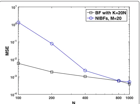
Figure1 displays the empirical MSE, averaged over 100 independent simulation runs, attained by the parallel schemes when the number of filters is fixed, M = 20, and the number of particles per filter (particle island) ranges fromN = 100 toN = 1000. The outcome of the
Fig. 1Empirical mean of the MSE for the centralised BF, with
K = MNparticles, and the ensemble of NIBFs, withM = 20 constant andN = 100, 200, 400, 800, 1000. All curves have been obtained from a set of 100 independent simulation trials. Note that the centralised BF is run withK = 20Nparticles, whereNtakes values in the same way as for the parallel algorithm
centralised BF withK = MN particles, hence ranging fromK = 20×100 toK = 20×1000, is also shown for comparison. We observe that proposed ensemble of NIBFs achieves a poor performance when the number of particles per filter,N, is relatively low (N = 100), while for moderate values (N ≥ 400) it nearly matches the MSE of the centralised BF.
Next, we look into the relationship between the MSE and the running time for the two algorithms. With the number of filters M = 20 fixed, we have run 100 independent simulation trials for each value N = 100, 200, 400, 800 and 1000 and computed the empirical MSE and the average running time for the parallel scheme and each combination ofMandN. Correspondingly, we have also run the centralised BF withK = MNparticles, hence forK=2×10³, 4×10³, 8×10³, 16×103and 20×103.
Figure2displays the resulting empirical MSE versus the running time for the two methods. If we qualify an algo-rithm as more efficient than another one when it is capa-ble of attaining a lower MSE in the same amount of time, then this set of simulations shows that the independent ensemble scheme is more efficient than the centralised BF. Indeed, a close look at Fig.2reveals that the ensemble of M=20 NIBFs withN=1000 particles per filter achieves an empirical MSE of≈ 6 × 10⁻⁴with a running time of ≈ 2.9 s, while the centralised BF attains the same perfor-mance withK = 20 × 800 particles and a running time of≈ 27.2 s (as shown by the dashed horizontal line in the plot).
5.2 Example: Lorenz 96 model
5.2.1 The J-dimensional Lorenz 96 system
The Lorenz 96 model is a deterministic system of non-linear differential equations that displays chaotic dynam-ics [33, 34]. The system dimension, i.e. the number of dynamic variables, can be scaled arbitrarily. A stochastic version of the model can be easily obtained by convert-ing each differential equation into a stochastic differ-ential equation driven by an independent and additive Wiener process. In particular, a model withJvariables,Zj,
j = 0,. . .,J−1, can be written down as the system of
whereF = 8 is a constant forcing parameter5, the Wiener processes {Wj(s)}l,j≥0 are assumed independent and the
scale parameterσis known.
A straightforward application of the Euler-Maruyama integration method yields a discrete-time version of the stochastic, two-scale Lorenz 96 model. If we letTd > 0
denote the discretisation period and n denotes discrete time, then we readily obtain
Zj,n=Zj,n−1−Td
and identically distributed (i.i.d.) standard Gaussian r.v.’s. We assume that observations can only be collected from this system once everyn0discrete time steps. Moreover,
only the variables with even indices (j = 0, 2, 4,. . .,J, for evenJ) are measured. Therefore, the observation process has the form
a J2-dimensional Gaussian distribution with 0 mean and covariance matrixσy2IJ
2.
Equations 35 and (36) describe a state space model that can be expressed in terms of the general nota-tion in Secnota-tion 2. The state process at time t is
˜ Xn =
%
Z0,n,. . .,ZJ−1,n
&
and the transition kernel from timen−1 to timenis
: RJ → RJ is the deterministic transformation that
accounts for all the terms on the right hand side of (35)
except the noise contribution √TdσUj,n. Since we only
collect observations every n0Td continuous-time units,
we need to put the dynamics of the states on the same time scale as the observation process{Yt}t≥1in Eq. (36). If we
We have run 100 independent simulations of the discre-tised Lorenz 96 model described in Section5.2.1above over 20 continuous-time units, with integration stepTd=
2×10⁻⁴(which amounts to 105discrete-time steps) and, for each simulation, we have obtained noisy observations, with σy2 = 12 and n0 = 10, according to Eq. (36). The
noise-scale parameter σ in the state Eq. (35) is set as σ = √1
2, so that the noise variance becomesσ 2
x = T2d.
The computer experiments are similar to Section 5.1. For each simulation, we have runM = 10 iNIBFs with N particles each versus a centralised BF withK = 10N particles and used them to compute one-step-ahead pre-dictions of the observations. In particular, at discrete-time t, we have computed predictions of the observation vector yt, using the measures
ξK
for the centralised BF and the NIBFs, respectively. To be specific, if yt =
y0,t,y1,t,. . .,yJ
2,t
resulting empirical MSE with respect to the observation
power 2J
J
2
r=0E
%
y2r,t&. Note that, in this case, we have used the actual observations generated in the simula-tions to obtain the errors, instead of the proxy values in Section5.1.
The experiments have been carried out for a Lorenz 96 model withJ = 20 variables first and then for the same model withJ=50 variables.
The simulations have been coded using Matlab ver-sion R2016b (64 bits), with the parallel computing toolbox enabled, on an 8-core Intel(R) Xeon(R) CPU E5-2680 v2 server, with clock frequency 2.80 GHz and 64 GB of RAM. All the results reported are averaged over 100 indepen-dent simulation runs as described above.
5.2.3 Numerical results
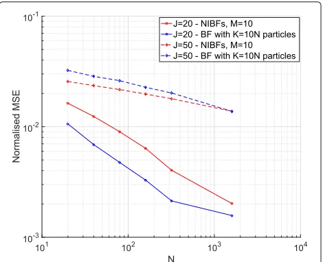
Figure3plots the normalised MSE attained by the cen-tralised BF and the ensemble ofM=10 NIBFs versusN. The centralised BF is run withK = 10N particles, while each one of theM=10 NIBFs is run withNparticles. The figure shows results for two different state-space dimen-sions. The solid lines correspond to a stochastic Lorenz 96 model with J = 20 variables. In this case, the out-come of the simulations is similar to the experiments with the Lorenz 63 system: forK = MN, the centralised BF attains a smaller MSE than the NIBFs, with the gap closing asN increases. The result of the experiment is different when the state space dimension is incremented toJ=50. In this case, the normalised MSE of the NIBFs is slightly smaller than the error of the centralised BF forN<1600,
Fig. 3Empirical mean of the normalised MSE for the centralised BF, withK=10Nparticles, and the average ofM=10 NIBFs with
N=20, 40, 80, 160, 320, 1600. Results are shown for a Lorenz 96 system withJ=20 variables (solid lines) and a Lorenz 96 model with
J=50 variables (dashed lines). All curves have been obtained from a set of 100 independent simulation trials
with both estimators attaining the same performance for N = 1600. Hence, for this example, the averaging of the NIBFs has a beneficial effect on the accuracy of the esti-mators, at least for certain combinations of the number of particlesNand the dimensionJ. We have verified that the bias of the centralised estimatoryKt is lesser than the bias of the estimatoryMt ×N, as predicted by the theoretical analysis, whileyMt ×N attains a smaller empirical variance thanyKt (at least forN<1600 and 40≤J≤100).
Figure 4 displays the results of the same computer experiment as in Fig.3, except that instead of averaging the MSE over the 100 independent simulation ruins, we display the maximum MSE, both for the centralised BF and the ensembles of NIBFs, out of the 100 simulations for each one of the values ofN. We observe that the ensem-ble of NIBFs is more robust than the centralised BF. While for dimensionJ = 20 the centralised BF attains a clearly lower average MSE than the NIBFs, the maximum MSE turns out to be similar for both algorithms. For dimension J = 50, the average MSE of the NIBFs is already lower (as shown in Fig.3) than the average MSE of the BF, and the advantage of the parallelised algorithm increases when we look at the maximum MSE.
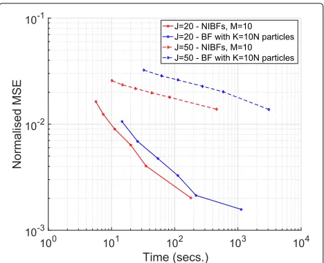
Figure5plots the same normalised MSE values of Fig.3 versus the running times of the algorithms, given in sec-onds, for a complete simulation with 105 discrete time steps. As in the experiments of Section5.1.3, the NIBFs can attain the same MSE as the centralised BF in just a fraction of the running time. While the improvement can be, ideally, of a factor M (with M = 10 in this case), in practice it depends on the efficiency of the computing software. With the version of Matlab (R2016b, with the