A fast inversion method for interpreting borehole electromagnetic data
Hee Joon Kim1, Ki Ha Lee2, and Michael Wilt3
1Pukyong National University, 599-1 Daeyeon-3-dong, Nam-Gu, Busan 608-737, Korea
2Ernest Orland Lawrence Berkeley National Laboratory, MS 90-1116, 1 Cyclotron Road, Berkeley, CA 94720, U.S.A. 3ElectroMagnetic Instruments, Inc., 1401 S. 46th St., UCRFS, Richmond, CA 94804, U.S.A.
(Received December 13, 2002; Revised May 10, 2003; Accepted May 11, 2003)
A fast and stable inversion scheme has been developed using the localized nonlinear (LN) approximation to analyze electromagnetic fields obtained in a borehole. The medium is assumed to be cylindrically symmetric about the borehole, and to maintain the symmetry a vertical magnetic dipole is used as a source. The efficiency and robustness of an inversion scheme is very much dependent on the proper use of Lagrange multiplier, which is often provided manually to achieve a desired convergence. We utilize an automatic Lagrange multiplier selection scheme, which enhances the utility of the inversion scheme in handling field data. In this selection scheme, the integral equation (IE) method is quite attractive in speed because Green’s functions, the most time consuming part in IE methods, are repeatedly re-usable throughout the selection procedure. The inversion scheme using the LN approximation has been tested to show its stability and efficiency using synthetic and field data. The inverted result from the field data is successfully compared with induction logging data measured in the same borehole.
Key words:Inversion, LN approximation, electromagnetic fields, borehole, cylindrical symmetry.
1.
Introduction
High-resolution imaging of electrical conductivity has been the subject of many studies in cross-hole tomography using electromagnetic (EM) fields (Zhouet al., 1993; Wiltet al., 1995; Alumbaugh and Morrison, 1995; Newman, 1995; Alumbaugh and Newman, 1997). Although the theoreti-cal understanding and associated field practices for cross-hole EM methods are relatively mature, these techniques are costly and sometimes it is difficult to find two adjacent bore-holes for cross-hole surveys. The cost can be greatly reduced if a single-hole survey method could be developed. Zhdanov and Gribenko (2002) discussed the problem of interpretation of a single-hole EM data.
The main advantage of integral equation (IE) method over the finite difference (FD) and/or finite-element (FE) methods is its greater suitability for inversion. For example, IE for-mulation readily contains a sensitivity matrix, which can be revised at each inversion iteration at little expense. With the FD or FE method, in contrast, the sensitivity matrix has to be recomputed at each iteration at a cost nearly equal to that of full forward modeling. The IE method, however, has to over-come severe practical limitations imposed on the size of the anomalous domain for inversion purposes. In this direction, several approximate methods such as the localized nonlinear (LN) approximation (Habashyet al., 1993) and quasi-linear approximation (Zhdanov and Fang, 1996) have been devel-oped. Recently, Leeet al.(2002) used the LN approximation for a cylindrically symmetric model to analyze single-hole EM data.
In this paper an advantage of the LN approximation is
Copy right cThe Society of Geomagnetism and Earth, Planetary and Space Sciences (SGEPSS); The Seismological Society of Japan; The Volcanological Society of Japan; The Geodetic Society of Japan; The Japanese Society for Planetary Sciences.
exploited with applications to inversion of borehole EM data. We begin our discussion with a critical check of the accuracy of LN approximation for a cylindrically symmetric model. We then describe our inversion algorithm and demonstrate the stability and effectiveness of this approach by inverting synthetic data. Finally, we present an example application to field data measured as a part of the Lost Hills CO2 pilot
project in southern California, U.S.A.
2.
LN Approximation
The LN approximation of IE solutions for a cylindrically symmetric model is described in detail in Leeet al.(2002). For completeness, their algorithm is briefly outlined here.
Assuming ane+iωt time dependency and neglecting
dis-placement currents, an IE solution for the electric fieldE(r)
atrcan be written by (Hohmann, 1975)
E(r)=Eb(r)−iωμ
V
GE(r−r)·σ(r)E(r)dv, (1)
whereEb(r)is the background electric field,GE(r−r)the
Green’s tensor,σ the conductivity,ωthe angular frequency, andμthe magnetic permeability. In Eq. (1),σ inside the integral means the excess conductivity, and the term σE
is called the scattering current (Hohmann, 1975). To obtain a numerical solution, the anomalous body is usually divided into a number of cells, and a constant electric field is as-signed to each cell (Hohmann, 1988). The process involved in volume IE methods requires computing time proportional to the number of cells used, and it quickly becomes imprac-tical as the size of inhomogeneity is increased to handle re-alistic problems.
For some important class of problems the complexity as-sociated with a full three-dimensional (3-D) problem can be
σ1 = 0.01 S/m z
ρ Mz
Hz
σ2 a
b 3 m
4 m
Fig. 1. A cylindrically symmetric model. The inhomogeneous body with a cross-section of 3 by 4 m is cylindrically symmetric about the borehole in which source (Mz) and receiver (Hz) are inserted. The parametersa andbrepresent the source-receiver and horizontal hole-body separations, respectively.
reduced to something much simpler. A model whose electri-cal conductivities are cylindrielectri-cally symmetric in the vicinity of a borehole is such an example. In order to preserve the cylindrical symmetry in the resulting EM fields, a horizon-tal loop current source or a vertical magnetic dipole may be considered in the borehole. In this case the problem is scalar when formulated using the azimuthal electric field Eϕ. The resultant IE solution is
Eϕ(r)=Eϕb(r)−2πiωμ
ρz
·GE(r−r)σ(r)Eϕ(r)ρdρd z, (2)
wherer= ρ+zandr= ρ+zare the position vectors, and the electric field and Green’s function are both scalar. The Green’s function is given in the form of a Hankel transform as (Ward and Hohmann, 1988, p. 219)
GE(r−r)= −
1
4π ∞
0
e−ub|z−z|
ub
λJ1(λρ)J1(λρ)dλ, (3)
where ub = (λ2 +iωμσb)1/2. Since measurements are
usually made for magnetic fields, Eq. (2) is modified as
Hz(r)=Hzb(r)−2πiωμ
ρz
·GH(r−r)σ(r)Eϕ(r)ρdρd z, (4)
whereGH(r−r)is the magnetic Green’s function, which
translates the scattering current σ(r)Eϕ(r) at r to the magnetic field atr.
Using Eqs. (2) through (4), we can obtain an IE solu-tion by first dividing a(ρ,z)cross-section into a number of cells, and formulate a system of equations for the electric field using a pulse basis function. Sena and Toksoz (1990) presented a crosshole inversion study for permittivity and conductivity in cylindrically symmetric medium using high-frequency EM, and Alumbaugh and Morrison (1995) inves-tigated crosshole EM tomography using an iterative Born ap-proximation and LN apap-proximation of Habashyet al.(1993).
The LN approximation offers an efficient and reasonably accurate electric field solution without deriving the full IE solution (Habashy et al., 1993). For the type of problem where there is only the azimuthal electric field, a good ap-proximation to Eq. (2) is given by (Leeet al., 2002)
Eϕ(r)≈γ (r)Eϕb(r), (5)
where
γ (r)=
1+2πiωμ
ρz
GE(r−r)σ(r)ρdρd z
−1
.
Substituting Eq. (5) into Eq. (4) yields an approximate magnetic-field solution
Hz(r)=Hzb(r)−2πiωμ
ρz
·GH(r−r)σ(r)γ (r)Eϕb(r)ρdρd z. (6)
To illustrate the efficiency and usefulness of the LN nu-merical solution, especially in a single-hole application, we consider a simple model consisting of a conductive ring about a borehole axis in a uniform 100 ohm-m whole space. The cross section of the ring is a 3 m by 4 m rectangle as shown in Fig. 1. Let us vary the transmitter-receiver offset (a in Fig. 1), borehole-to-conductor distance (b in Fig. 1), and the conductivity contrast(σ2/σ1)and find out how the
LN approximated vertical magnetic field compares with the result obtained from the full FE method (Leeet al., 2003). Unless otherwise indicated the frequency used is 100 kHz throughout.
Figure 2 shows a comparison in secondary vertical mag-netic fields between the FE (solid and dashed lines) and LN (symbols) solutions for three different transmitter-receiver separations: 4 m, 6 m, and 8 m. The center of the body is chosen as z = 0, and plots are made at the transmitter-receiver midpoint. The conductivity contrast used is 10, and the borehole-to-conductor distance is 3 m. For all separa-tions, the two solutions agree very well. More anomalies can be observed in the imaginary part. The anomaly also gets stronger for shorter source-receiver separations. At the sepa-ration of 4 m the imaginary part of the anomaly is 2.0×10⁻⁴
A/m, and it is about 8% of the primary field of 2.48×10⁻³
A/m (not shown here).
Next, we consider EM responses by varying the borehole-to-conductor separation, while the conductivity contrast and transmitter-receiver separation are fixed to 10 and 4 m, re-spectively. When the separation is small, it is anticipated that the LN approximation may not be as good, because the rapid change in electric fields in the vicinity of the transmit-ter is not a favorable condition for the LN approximation. Figure 3 confirms this is indeed the case. For the separation of 1 m, we can see significant difference in the peak values of the real part between the FE and LN solutions. The differ-ence is less in the imaginary part.
4 m 6 m 8 m
12 6 0 -6 -12
Real(Hzs) (x10-5 A/m)
-10 -8 -6 -4 -2 0
Imag.(Hzs) (x10-5 A/m)
12 6 0 -6 -12
z
(m)
-4 0 -8
-12 -16 -20
Fig. 2. The effect of source-receiver separation (ain Fig. 1) on the vertical component of secondary magnetic fields. Operating frequency is 105Hz. The 0.1 S/m body is located in a whole space of 0.01 S/m at 3 m horizontally away from the borehole (b=3 m in Fig. 1). The solid and dashed lines show exact solutions.
1 m 2 m 4 m
12 6 0 -6 -12
Real(Hzs) (x10-5 A
-10 -8 -6 -4 -2 0
Imag.(Hzs) (x10-4 A/m)
12 6 0 -6 -12
z
(m)
0 -1 -2 -3 -4 -5
/m)
Fig. 3. The effect of hole-body separation (bin Fig. 1) on the vertical component of secondary magnetic fields. The operating frequency is 105Hz, the conductivity contrast between body and background is 10, and the source-receiver separation (ain Fig. 1) is 4 m. The solid and dashed lines show exact solutions.
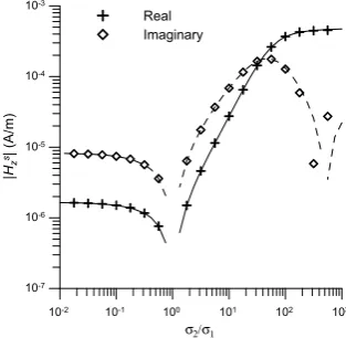
approximation is very well up to the conductivity contrast of 200 as shown in Fig. 4. The imaginary part of the LN solu-tion starts deviating from the FE solusolu-tion beyond the conduc-tivity contrast of 200, while the real part still shows a good agreement.
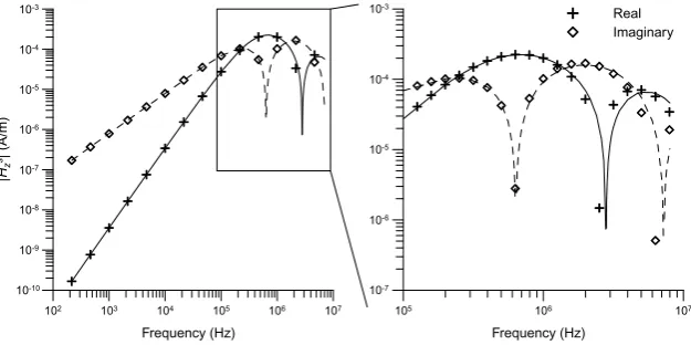
Finally, a comparison is made for magnetic responses in frequency (Fig. 5). The conductivity contrast, transmitter-receiver separation, and borehole-to-conductor distance are fixed to 10, 6 m, and 3 m, respectively, and FE and LN solutions are obtained for frequencies ranging from 200 Hz to 80 MHz. The two solutions show a good agreement all the way up to 2 MHz (see details on the right of Fig. 5).
3.
Inversion
Based on the encouraging results of the LN approxima-tion, we have proceeded to implement the inversion scheme for interpreting borehole EM data. Measurements are made in the same borehole as the transmitter, so the radial distance ρis zero. Upon dividing the inhomogeneity intoKelements, the secondary magnetic field at thei-th receiver position in the borehole may be written as
Hzis ≈ −2πiωμ
K
k=1
σkγkEϕbk
σ2/σ1
|
Hz
s| (A/m)
Real Imaginary
10-1
10-2 100 101 102 103
10-3
10-4
10-5
10-6
10-7
Fig. 4. The effect of conductivity contrast between body and background on the secondary magnetic fields. The operating frequency is 105 Hz, the source-receiver separation (a in Fig. 1) is 6 m and the horizontal hole-body separation (bin Fig. 1) is 3 m. The solid and dashed lines show exact solutions.
·
Sk
GH(ρ,zi−z)ρdρd z, (7)
Frequency (Hz) Real Imaginary
105 106 107
10-7
10-6
10-5
10-4
10-3
Frequency (Hz)
|
Hz
s| (A/m)
106
10-10
10-9
10-8
10-7
10-6
10-5
10-4
10-3
107
105
104
103
102
Fig. 5. The effect of operation frequency on the secondary magnetic fields. The source-receiver separation is 6 m. The 0.1 S/m body is located in a whole space of 0.01 S/m at 3 m horizontally away from the borehole. The solid and dashed lines show exact solutions.
deduced from the electric-field Green’s function (3) as
GH(ρ,zi−z)=
1
4πiωμ ∞
0
e−ub|z−z|
ub
λ2J
1(λρ)dλ
= − 1
4πiωμ ∂ ∂ρ
e−i kb|r−r| |r−r|
, (8)
wherekb =(−iωμσb)1/2. The secondary vertical magnetic
field along the borehole axis can be easily evaluated by sub-stituting Eq. (8) into Eq. (7), and performing integration in ρandz. For the inversion, the sensitivity of the magnetic field with respect to the change in conductivity can be easily obtained from Eq. (7). Taking derivative of magnetic fields with respect to the j-th conductivity parameter and neglect-ing the dependence ofγj onσj, the sensitivity becomes
∂Hs zi
∂σj
≈ −2πiωμγjEϕbj
Sj
GH(ρ,zi−z)ρdρd z, (9)
which can be easily evaluated by integrating over the j-th element.
The inversion procedure starts with a data misfit
Wd[H(σ)−Hd]|2, where · denotes the Euclidean norm
and the subscriptdrepresents data. The data weighting ma-trixWd is used to give relative weights to individual data. If
a perturbationδσ is allowed to the conductivity, the misfit takes a formWd[H(σ+δσ)−Hd]|2, and the total
objec-tive functional may be written as
φ= Wd[H(σ+δσ)−Hd]2+λWσδσ2, (10)
where the second term on the right-hand side is added to impose a smoothness constraint, and Wσ is the weighting matrix for model parameters andλis the Lagrange multiplier that controls the trade-off between data misfit and parameter smoothness. Expanding the misfit in δσ using the Taylor series, discarding terms higher than the square term, and letting the variation of the functional with respect toδσequal to zero, we can obtain a linear system of normal equations for the perturbationδσas
(JTWTdWdJ+λWTσWσ)δσ = −JTWTdWd[H(σ)−Hd],
(11)
where the superscriptT indicates matrix transpose, and the entries of Jacobian matrix J are the sensitivity functions given in Eq. (9).
The stability of the inversion is largely controlled by re-quiring the conductivity to vary smoothly. Larger values of λresult in smooth and stable solutions at the expense of res-olution. It even allows for the solution of grossly underde-termined problems (Tikhonov and Arsenin, 1977). In this single-hole inversion study, we employ the Occam approach, first proposed by Constableet al.(1987) (see also deGroot-Hedlin and Constable, 1990; Parker, 1994), to determine an optimum Lagrange multiplierλduring the inversion process. The unique feature of the Occam approach is that the param-eterλis used at each iteration both as a step length control and a smoothing parameter. That is, Eq. (11) is solved for a series of trial values ofλand the rms misfit for eachλis eval-uated by solving the 2-D forward problem. The Occam pro-cess thus chooses the model with the minimum misfit as the basis for the next iteration. The minimization can be carried out by means of a simple 1-D line search. In this selection scheme, the IE modeling is quite attractive in speed because Green’s functions for the electric field involving the Hankel transform, the most time consuming part in IE methods, are repeatedly re-usable throughout the selection procedure. In this study three times of forward modeling are conducted to select an optimum Lagrange multiplier at each iteration.
The conductivity model shown in the left of Fig. 6 is cho-sen to evaluate the performance of extended Born inversion using the LN approximation. The model consists of two cylindrically symmetric bodies, one conductive (1 S/m) and the other resistive (0.01 S/m), in a whole space of 0.1 S/m. A FE scheme (Leeet al., 2003) is used to generate synthetic data. The accuracy of the FE scheme is estimated as a level of less than 1% compared with the exact IE solution. Using a vertical magnetic dipole as a source, vertical magnetic fields are computed at five source-receiver offsets of 4 m through 8 m at three frequencies of 12 kHz, 24 kHz and 42 kHz. Using 3-digit synthetic data generated by the FE method, the inversion is started with an initial model of 0.25 S/m uniform whole space.
0 2 4 6 8 10 12
Fig. 6. Inversion of synthetic model. The model (left) used to calculate synthetic data for inversion test consists of two cylindrically symmetric bodies, of 1 S/m and 0.01 S/m, located in a whole-space of 0.1 S/m. An image of two conductors reconstructed from the synthetic data after 6th iteration.
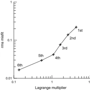
Fig. 7. Convergence in rms misfit and associated Lagrange multiplier as a function of iteration during the synthetic model inversion.
is found to be nearly the same in the conductive body but is overestimated in the resistive body. The initial model was chosen arbitrary but the inversion result was almost indepen-dent with the initial model. The inversion process is quite stable as shown in Fig. 7, where the rms misfit decreases from the initial guess of 0.478 (not shown in Fig. 7) to under 0.01 after 6 iterations. The rms misfit is given by the relative data misfit
where N is the number of data. The rms misfit of 0.01 is assumed to be a target misfit level because the error level in the synthetic responses is estimated to be about 1%. Also, as shown in Fig. 7, the smoothing parameter varies from 50
0 12 24
Fig. 8. Resistivity section (right) derived from the inversion of single-hole EM data and an apparent resistivity log (left) measured in the same borehole.
Fig. 9. Convergence in rms misfit and associated Lagrange multiplier during the inversion of field data.
to less than 0.2 during the inversion process. The change is significant, and this means it is difficult to determine the parameter a priori.
Finally, the 2-D inversion algorithm has been applied to a set of single-hole field data obtained as a part of the Lost Hills CO2 pilot project in southern California in May 2001
(Wiltet al., 2002). The EM data were measured with Geo-BILT, a newly built induction logging tool manufactured by Electromagnetic Instruments, Inc. Although the tool features a series of three-component sensors and a three-component source, onlyMz–Hz(vertical magnetic fields due to a
verti-cal magnetic dipole) data are utilized for this inversion ex-periment. The offsets between the source and receivers were 2 m and 5 m and the operating frequency was 6 kHz.
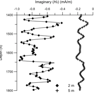
1800 1700 1600 1500 1400
Depth (ft)
Imaginary (Hz) (mA/m)
2 m 5 m
-1.0 -0.8 -0.6 -0.4 -0.2 0
Fig. 10. Comparison of field data (solid lines) and inverted model responses (diamonds and pluses) in the imaginary component.
produce a resistivity section shown on the right of Fig. 8. The inversion process is quite stable as shown in Fig. 9, where the rms misfit decreases from 0.307 (not shown in Fig. 9) for the initial guess to 0.017 after 6 iterations, while the correspond-ing smoothcorrespond-ing parameter is seen monotonically decreascorrespond-ing from above 40 to a little more than 0.1. Further reduction of rms misfit is possible at the expense of overfitting. Note that a target misfit level is not known for the field data. The fit of 2-D model responses to the field data is quite well as shown in Fig. 10, in which only the imaginary part is com-pared because the real part has very little anomaly. Due to the assumption of cylindrical symmetry the reconstructed image may be different from the real resistivity section especially in the far side from the borehole. The image near the borehole, however, is considered to be reasonable because it is compa-rable with an apparent resistivity log obtained from induction logging (Wilt and Alumbaugh, 1998) in the same borehole, shown on the left of Fig. 8. In particular, the resistive zone imaged around the borehole is quite similar with the logging result. Computing time required for the 2-D approximate in-version is about 10 minutes on a Pentium-4 1.5 GHz PC to obtain 539 conductivities from 534 complex Hz fields after
6 iterations.
4.
Conclusions
The extended Born or LN approximation of IE solution has been applied to inverting single-hole EM data using a cylindrically symmetric model. The LN approximation is less accurate than a full solution but much superior to the simple Born approximation. Moreover, when applied to the cylindrically symmetric model with a vertical magnetic dipole source, the accuracy of LN approximation is greatly improved because electric fields are scalar and continuous everywhere. One of the most important steps in the inver-sion is the selection of a proper regularization parameter for stability. The LN solution provides an efficient means for selecting an optimum regularization parameter, because Green’s functions, the most time consuming part in IE meth-ods, are repeatedly re-usable throughout inversion. In addi-tion, the IE formulation readily contains a sensitivity matrix, which can be revised at each iteration at little expense. This fast inversion scheme has been tested on its stability and
ef-fectiveness using synthetic and field data. The reconstructed image from the field data was comparable with resistivity logging data.
Acknowledgments. This research was supported by Korea Sci-ence and Engineering Foundation (R01-2001-000-000071-0). The collaboration by the second author was partially supported by the Assistant Secretary for Energy Efficiency and Renewable Energy, Office of Wind and Geothermal Technologies of the U.S. Depart-ment of Energy under Contract No. DE-AC03-76SF00098. We would like to thank Michael Morea, Chevron USA Production Company, and the US Department of Energy, National Petroleum Technology Office, (Class III Field Demonstration Project DE-FC22-95BC14938) for allowing us to publish this data. We would like to thank Editor and reviewers for their valuable suggestions and comments in improving the quality of this paper.
References
Alumbaugh, D. L. and H. F. Morrison, Theoretical and practical consider-ations for crosswell electromagnetic tomography assuming a cylindrical geometry,Geophysics,60, 846–870, 1995.
Alumbaugh, D. L. and G. A. Newman, Three-dimensional massively paral-lel electromagnetic inversion (II. Analysis of crosswell electromagnetic experiment,Geophys. J. Int.,128, 355–363, 1997.
Constable, S. C., R. L. Parker, and C. G. Constable, Occam’s inversion: A practical algorithm for generating smooth models from electromagnetic sounding data,Geophysics,52, 289–300, 1987.
deGroot-Hedlin, C. and S. Constable, Occam’s inversion to generate smooth, two-dimensional models from magnetotelluric data,Geophysics, 55, 1613–1624, 1990.
Habashy, T. M., R. M. Groom, and B. R. Spies, Beyond the Born and Rytov approximations: a nonlinear approach to electromagnetic scattering,J. Geophys. Res.,98, 1795–1775, 1993.
Hohmann, G. W., Three-dimensional induced polarization and EM model-ing,Geophysics,40, 309–324, 1975.
Hohmann, G. W., Numerical modeling for electromagnetic methods of geophysics, inElectromagnetic Methods in Applied Geophysics,Vol. 1, edited by M. N. Nabighian, pp. 313–363, Soc. Expl. Geophys., 1988. Lee, K. H., H. J. Kim, and M. Wilt, Efficient imaging of single-hole
elec-tromagnetic data,Geothermal Resources Council Transactions,26, 399– 404, 2002.
Lee, K. H., H. J. Kim, and T. Uchida, Electromagnetic fields in steel-cased borehole,Geophys. Prosp., 2003 (submitted).
Newman, G. A., Crosswell electromagnetic inversion using integral and differential equations,Geophysics,60, 899–911, 1995.
Parker, R. L.,Geophysical Inverse Theory,Prinston Univ. Press, 1994. Sena, A. G. and M. N. Toksoz, Simultaneous reconstruction of permittivity
and conductivity for crosshole geometries,Geophysics,55, 1302–1311, 1990.
Tikhonov, A. N. and V. Y. Arsenin,Solutions to Ill-Posed Problems,John Wiley and Sons, Inc., 1977.
Ward, S. H. and G. W. Hohmann, Electromagnetic Theory for Geophysical Applications, inElectromagnetic Methods in Applied Geophysics,Vol. 1, edited by M. N. Nabighian, pp. 131–311, Soc. Expl. Geophys., 1988. Wilt, M. J. and D. L. Alumbaugh, Electromagnetic Methods for
Develop-ment and Production: State of the Art:The Leading Edge,17, 487–490, 1998.
Wilt, M. J., D. L. Alumbaugh, H. F. Morrison, A. Becker, K. H. Lee, and M. Deszcz-Pan, Crosshole electromagnetic tomography: System design considerations and field results,Geophysics,60, 871–885, 1995. Wilt, M., R. Mallan, P. Kasameyer, and B. Kirkendahl, Extended 3D
induc-tion logging for geothermal resource assessment: Field results with the Geo-BILT system, Proc. 27th Stanford Geothermal Workshop, Stanford Univ., SGP-TR-171, 2002.
Zhdanov, M. S. and S. Fang, Quasi-linear approximation in 3-D EM model-ing,Geophysics,61, 646–665, 1996.
Zhdanov, M. S. and A. Gribenko, Three-dimensional imaging about a sin-gle borehole, 72nd Ann. Internat. Mtg., Soc. Expl. Geophys., Expanded Abstracts, 316–319, 2002.
Zhou, Q., A. Becker, and H. F. Morrison, Audio-frequency electromagnetic tomography in 2-D,Geophysics,58, 482–495, 1993.