Probability gains expected for renewal process models
Masajiro Imoto
National Research Institute for Earth Science and Disaster Prevention, Tennodai 3-1, Tsukuba-shi, Ibaraki-ken 305-0006, Japan
(Received February 12, 2004; Revised April 27, 2004; Accepted May 17, 2004)
We usually use the Brownian distribution, lognormal distribution, Gamma distribution, Weibull distribution, and exponential distribution to calculate long-term probability for the distribution of time intervals between successive events. The values of two parameters of these distributions are determined by the maximum likelihood method. The difference in log likelihood between the proposed model and the stationary Poisson process model, which scores both the period of no events and instances of each event, is considered as the index for evaluating the effectiveness of the earthquake probability model. First, we show that the expected value of the log-likelihood difference becomes the expected value of the logarithm of the probability gain. Next, by converting the time unit into the expected value of the interval, the hazard is made to represent a probability gain. This conversion reduces the degrees of freedom of model parameters to 1. We then demonstrate that the expected value of the probability gain in observed parameter values ranges between 2 and 5. Therefore, we can conclude that the long-term probability calculated before an earthquake may become several times larger than that of the Poisson process model.
Key words:Probability gain, information gain, renewal model, Kull-back Leibler, long-term probability, Gamma, Brownian, Weibull.
1.
Introduction
Many seismologists contend that deterministic prediction of earthquakes is impossible. Probability values of earth-quake predictions are widely used to forecast occurrences. Long-term probabilities using renewal processes were pub-lished in California for earthquakes along the San Andreas Fault (Working Group on California Earthquake Probabil-ties, 1988) and the San Francisco Bay region (Working Group on California Earthquake Probabilties, 1990). The probabilities for thrusting earthquakes along the Japanese trench, including offshore Miyagi Prefecture and along in-land active faults in Japan, were estimated by the Earthquake Research Committee (2000, 2002).
A high probability for a narrow and limited time-spatial area that includes the time of an earthquake and its hypocen-ter is useful in earthquake probabilistic predictions. The method currently used to estimate long-term probability is based on a renewal process model, a point process (Utsu, 1984). A specific period and time are assumed in probability calculations based on the point process, and the probability of an earthquake is evaluated. Therefore, the probability de-pends on the size of the object space-time; the probability in-creases as the object space time is increased. In some cases, it is possible to approximate the probability to 1. Therefore, both the probability and the size of the object space-time are important considerations. Investigating any deviation from the average probability is a reasonable means of evaluating a method’s effectiveness in determining the probability of an earthquake. The concept of probability gain is important,
Copy right cThe Society of Geomagnetism and Earth, Planetary and Space Sciences (SGEPSS); The Seismological Society of Japan; The Volcanological Society of Japan; The Geodetic Society of Japan; The Japanese Society for Planetary Sciences; TERRA-PUB.
since probability gain is defined as the ratio of probability to that of a steady Poisson model and therefore is not directly affected by the size of the space-time in a probability calcu-lation.
Kagan and Knopoff (1987) introduced the information content, which is the base 2 logarithm of the likelihood ra-tio of a particular model to the Poisson model. By divid-ing the information content by the number of earthquakes, they defined an information content ratio. They regarded this quantity as an estimate of effectiveness of predictions, where they evaluated their model for short-term prediction based on clustering features of earthquakes. Imoto (2000, 2001) reported that the difference in log-likelihood between the proposed model and the Poisson model is the logarithm of the product of probability gains. He also indicated that the value obtained by dividing the difference in log-likelihood by the number of earthquakes is an index for assessing ef-fectiveness. Therefore, we focus on this quantity for evalu-ating the potential of the long-term predicting method using the renewal process model. We will clarify the limit of the long-term method in terms of probability gain by theoreti-cally estimating the quantity over a wider range of parameter values than those obtained in practical cases.
2.
Formulation
Prediction validity is commonly assessed using a point-process model by means of the difference between the log-likelihood of the pertinent model and the log-log-likelihood of the stationary Poisson model (Evison and Rhoades, 1993; Imoto, 1994). When the model is optimized for existing ob-served values, the value obtained by dividing the difference in log-likelihood by the number of earthquakes is the geo-metrical mean of the probability gains for individual earth-quakes (Vere-Jones, 1998; Imoto, 2001). The difference
tween log-likelihood as the base in accordance with this con-cept will be calculated, and this paper will demonstrate that it is equivalent to the expected value of probability gain.
Using the earthquake that occurred first as the reference, we assume thatnearthquakes occurred subsequently at inter-vals ofτ1,τ2,τ3,. . .,τn. These are mutually independent and identically distributed random variables. Let F(t)be their distribution function,
F(t)= P(τi <t), (1)
where the right side of Eq. (1) gives a probability that arbi-trary selected time interval,τi , is less thant, and f(t)is its is called the reliability function. The hazard functionμ(t)is defined with the relation
μ(t)= f(t)
φ(t) (4)
or
μ(t)= −d
dtlnφ(t) (5)
Here and hereafter, ln refers to the natural logarithm. In general, the log-likelihood 1 for the hazard function, λ(t), in the interval 0 toT, can be expressed as follows:
l = −
is established. Then the following relation will be obtained:
n
Considering the log-likelihood per earthquake asl1, this can be expressed as follows:
l1 = 1
Provided thatn is sufficiently large, the average operation can be replaced with the following integral:
l1= −
Using these relations, Eq. (11) can be rewritten as follows:
1 = −
In contrast, it is expressed as follows in the stationary Pois-son process:
λ= n
T (13)
The log-likelihood for this process,lpis given as:
p = −
Here,T¯ =T/n. Therefore, the difference in log-likelihood per earthquake can be expressed as follows:
1−1 p=
∞
0
f(τ)lnμ(τ)dτ +lnT¯ (16)
When the average value of intervals between earthquakes,T¯, is set as the unit on the time axis, the following expression can be obtained by replacing f(τ),μ(τ)with f(τ),μ(τ)
where we can use the relations
F(τ)=F(T¯τ)
and
f(τ)= ¯T f(T¯τ).
This value corresponds to the Kullback-Leibler quantity of information (Sakamoto et al., 1983), which represents the difference between the two distributions (see the appendix). Hereinafter, a function or variable with an underscore mark will mean that the unit of time is transformed into the average time interval. Furthermore, the left side of Eq. (17) will be called the Information Gain per event (IGpe) (Daley and Vere-Jones, 2003), which is equivalent to the average of probability gain (right side). The model parameter of f(τ) will satisfy the following relation:
¯
T =1=
∞
0
t f(t)dt (18)
In this study, Eq. (17) was integrated numerically.
3.
Expectance of Probability Gains
Table 1. List of information gains and IGpe for six characteristic earthquake sequences. Each information gain is converted from the respective AIC value given in the report (Earthquake Research Committee, 2001), where the Poisson model is taken as a baseline.
Brownian Lognormal Gamma Weibull Exponential
Nankai trough 5.45 5.40 5.25 4.95 4.25
(Nan) 0.68 0.68 0.66 0.62 0.53
off-shore of Miyagi 6.65 6.65 6.80 7.60 7.90
Prefecture (Miy) 1.33 1.33 1.36 1.52 1.58
Atera Fault 4.30 4.30 4.60 5.40 5.85
(Ate) 0.86 0.86 0.92 1.08 1.17
Atotsugawa Fault 5.60 5.60 5.60 5.45 5.30
(Ato) 1.40 1.40 1.40 1.36 1.33
Tanna Fault 5.80 5.80 5.90 6.25 6.25
(Tan) 1.16 1.16 1.18 1.25 1.25
Western margin of 8.10 8.10 8.00 7.65 7.10
the Nagano basin (Nag) 1.01 1.01 1.00 0.96 0.89
Table 2. List of time intervals (in years) for the six sequences, intervals of which are used for estimating IGpe (Table 1) and model parameters (Table 3) (Earthquake Research Committee, 2001).
Nankai trough off-shore of Atera Fault Atotsugawa Fault Tanna Fault Western margin of
Miyagi Prefecture the Nagano basin
202.7 42.4 1009.5 2291 1320 1019
211.5 26.3 2246 3066 1460 1581
262.4 35.3 2092 2570 1172 818
136.9 39.7 1982 1957.5 788 1247.5
106.6 41.6 1742 1089 1385.5
102.7 823.5
147.2 779
92.0 1111.5
Average 157.8 37.1 1814.3 2471.1 1165.8 1095.6
widely adopted because it is easy to understand as a model of the accumulation of stress and the disturbance of stress fields. Each of these distributions contains two model pa-rameters. The two parameters,θ1 andθ2are determined by the maximum likelihood method so that they can be adapted to the observed time intervals. As an example of practical cases, information gain (Table 1) is calculated, using time intervals in Table 2 for six characteristic sequences, where the model parameters of the above mentioned distributions are estimated by the maximum likelihood method (Table 3) (Earthquake Research Committee, 2001). The IGpe value obtained from each distribution can be calculated as follows:
3.1 Brownian model
The functions of f(t), φ(t)andμ(t)are expressed in this model by the following designations:
f(t)=
The expected time interval value is equal toθ1(Matthews
et al., 2002). Therefore, conversion of the unit of time that
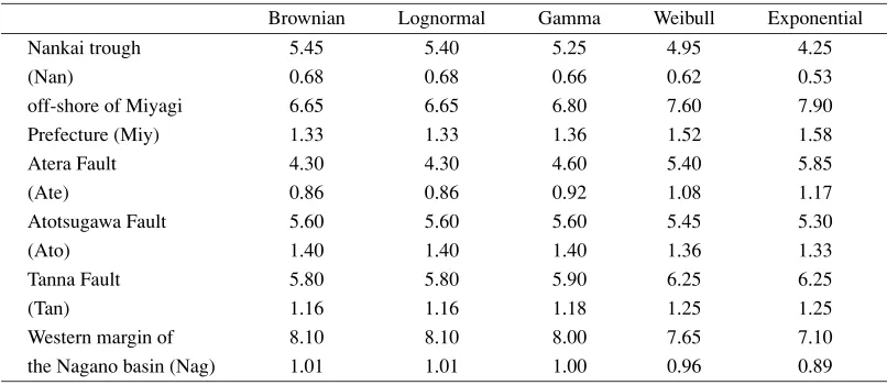
meets the conditions in Eq. (18) can be accomplished by defining θ1 = 1. The IGpe value obtained by varying the other parameter,θ2, within the range of 0.055 to 0.5 is drawn in Fig. 1. The scale of IGpe is given on the left side of the vertical axis, and the probability gain is indicated on the right side. The IGpe value varies from 0.3 to 2.4 withθ2varying and the probability gain value varies from 1.4 to 10. The value ofθ2was obtained within the range of 0.16 to 0.37 in a previous research (Table 3), which corresponds to the range of probability gain from 2 to 4.
Brownian
0.0
0.1
0.2
0.3
0.4
0.5
0.00
1.00
2.00
3.00
4.00
1.0
2.0
5.0
10.0
20.0
50.0
Nan Miy
Ato Tan Nag Ate IGpe
Prob.Gain
Fig. 1. Variation of IGpe withθ2varying from 0.05 to 0.5 for the Brownian model. Triangles indicate values obtained from the cases in Table 1 (Ate,
Atera; Ato, Atotugawa; Miy, Miyagi; Nag, Nagano; Nan, Nankai; Tan, Tanna). The left and right sides of the scale indicate IGpe and probability gain.
lognormal
0.0
0.1
0.2
0.3
0.4
0.5
0.00
1.00
2.00
3.00
4.00
1.0
2.0
5.0
10.0
20.0
50.0
Nan Miy
Ato Tan Nag Ate
IGpe Prob.Gain
Fig. 2. Variation of IGpe withθ2varying from 0.05 to 0.5 for the lognormal model. See Fig. 1 for triangles and both sides of the scales.
3.2 Lognormal model
The functions of f(t), φ(t)andμ(t)are presented in this model by the following designations:
f(t)= √ 1
2πθ2t exp
−(lnt−θ1) 2θ2
2
(22)
φ(t)=1−
lnt−m
θ2
(23)
μ(t)=√ 1 2πθ2t exp
−(lnt−θ1)2 2θ2
2
φ(t) (24)
The expected value of the time interval, T¯, is expressed as follows:
¯
T =exp
θ1+
θ2 2 2
(25)
Therefore, the following relation can be obtained from the conditions in Eq. (18):
θ1= −θ 2 2 2
Gamma
0.
10.
20.
30.
40.
50.
0.00
1.00
2.00
3.00
4.00
1.0
2.0
5.0
10.0
20.0
50.0
Nan Ate Nag Tan Miy Ato
IGpe 1
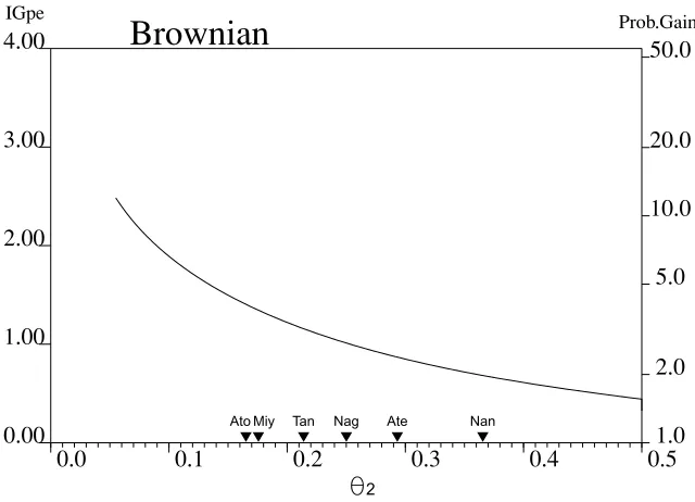
Fig. 3. Variation of IGpe withθ2varying from 0.5 to 50. for the Gamma model. See Fig. 1 for triangles and both sides of the scales.
Conversion of the unit of time in this model only af-fects parameterθ1without affectingθ2, as with the Brownian model. Therefore, the IGpe and probability gain values can be obtained directly from Fig. 2 using the value of parameter
θ2when two parameters are estimated in a practical case.
3.3 Gamma model
The functions of f(t), φ(t) and μ(t) are given in this model by the following designations:
f(t)=θ
θ2
1 tθ2−1e−θ1 t
(θ2)
(26)
φ(t)= (θ2, θ1t)
(θ2)
(γ,x)=
∞
x
e−uuγ−1du (27)
μ(t)= θ
θ2
1 tθ2−1e−θ1 t
(θ2, θ1t)
(28)
The expected value of time interval T¯ is expressed as follows (Utsu, 1999):
¯
T =θ2
θ1
(29)
Therefore, the variation of the IGpe value with varying θ2 within the range of 1< θ2 <50, assuming thatθ1 =θ2, is shown in Fig. 3. The value ofθ2was obtained within a range of 7.9 to 37 for the cases in Table 3. The probability gain would then be within the range of 1.9 to 4.1. The IGpe value would then be 0 forθ2 =1, since this model is compatible to the Poisson model. This model with θ2 less than 1.0 presents a power-law decay with time, which corresponds to an expression of the clustering feature of earthquakes. The value ofθ2 would not be affected by conversion of the unit of time in this model, similar to the above two models. Therefore, the IGpe and probability gain can be obtained directly from Fig. 3 using the value of parameter θ2 when two parameters are estimated in a practical case.
3.4 Weibull model
The functions of f(t), φ(t)andμ(t)are expressed in this model by the following designations:
f(t)=θ1θ2tθ2−1exp
−θ1·tθ2
(30)
φ(t)=exp−θ1tθ2 (31)
μ(t)=θ1θ2tθ2−1 (32)
The expected value of time interval T¯ is expressed as follows:
¯
T = 1
θθ12 1 ·θ2
1
θ2
(33)
An equation in whichθ1in Eq. (30) is replaced with
1
θ2
1
θ2
θ2
(34)
will be derived to express the distribution of t when the conversion oft=T tis implemented, and thus the condition of T = 1 is met. The parameter θ2 is kept unchanged throughout this conversion; the IGpe value using parameter
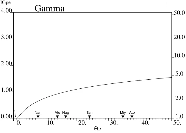
θ2 within a range of 0.3 < θ2 < 10 is shown in Fig. 4. The value of θ2 was obtained within a range of 3.0 to 8.9 (Table 3). The probability gain would then be within a range of approx. 1.8 to 5.0. This model is compatible to the Poisson model whenθ2 =1, and thus the value of IGpe is equal to be 0. This model with θ2 less than 1.0 presents a power-law decay with time for the clustering feature of earthquakes, similar to the Gamma model.
Weibull
0.
2.
4.
6.
8.
10.
0.00
1.00
2.00
3.00
4.00
1.0
2.0
5.0
10.0
20.0
50.0
Nan Nag Ate TanAto Miy
IGpe Prob.Gain
Fig. 4. Variation of IGpe withθ2varying from 0.3 to 10. for the Weibull model. See Fig. 1 for triangles and both side scales.
3.5 Exponential model
The functions of f(t), φ(t) and μ(t) are given in this model by the following designations:
f(t)=θ1exp
θ1
1−eθ2·t
θ2
+θ2·t
(35)
φ(t)=exp
θ
1
θ2
1−eθ2·t (36)
μ(t)=θ1exp(θ2t) (37) The expected value of time intervalT¯ is given as follows:
¯
T = −exp
θ1
θ2
· 1
θ2
Ei
−θ1
θ2
(38)
Here,
Ei(x)=
x
−∞
eu
u du (39)
The values ofθ1andθ2will be obtained when the follow-ing relations are assumed for the conversion oft = ¯T t,
θ1= ¯Tθ1 (40)
θ2= ¯Tθ2. (41) The following relation will then be obtained:
θ1
θ2
= θ1
θ2
The IGpe value using parameterθ2/θ1within the range of 1 to 1.0×10⁵ is shown in Fig. 5. The value ofθ2/θ1 was obtained within the range of 15 to 2×10⁴in Table 3. The probability gain would then be within the range of approx. 1.6 to 5.4. This model tends to the Poisson model asθ2 ap-proach to 0, so the IGpe value would be 0. The IGpe and probability gain values for this model can be obtained from
Fig. 5 using the value of parameterθ2/θ1 when two param-eters are estimated in a practical case, unlike the preceding four models.
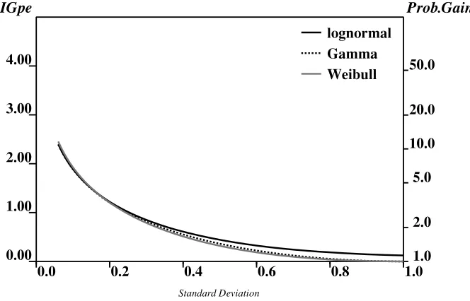
The above analysis of IGpe shows that parameters re-lated to a variance of time intervals play substantial roles in estimating IGpe. To confirm this feature, the IGpes are shown as a function of the standard deviation for log-normal, Gamma, and Weibull models (Fig. 6). The stan-dard deviation here stands for the stanstan-dard deviation divided by the mean time interval, since the time unit is normal-ized to the mean time interval. The standard deviations for these models are analytically derived as
exp(θ2 2)−1,
1√θ2 and
(2/θ2+1) /{ (1/θ2+1)}2−1 for log-normal, Gamma, and Weibull models (Utsu, 1999). In the figure, only a part of the standard deviation less than 1 is shown since that is the case for the quasi-periodic feature, which is the base of long-term probability assessment. It is obvious that differences among the three curves are small. The Brownian and the exponential models are much more similar to those of the lognormal and Gamma models. There-fore, the charts for these models are not shown here.
4.
Summary
fluctua-Exponential
0.1E+01 0.1E+02 0.1E+03 0.1E+04 0.1E+05 0.1E+06
0.00
1.00
2.00
3.00
4.00
1.0
2.0
5.0
10.0
20.0
50.0
Nan Nag TanAteAto Miy
IGpe Prob.Gain
Fig. 5. Variation of IGpe withθ2/θ1varying from 1 to 105for the exponential model. See Fig. 1 for triangles and both side scales.
0.0 0.2 0.4 0.6 0.8 1.0
0.00 1.00 2.00 3.00 4.00
1.0 2.0 5.0 10.0 20.0 50.0 lognormal Gamma Weibull
IGpe
Prob.Gain
Standard Deviation
Fig. 6. Variation of IGpe with standard deviation varying from 0.05 to 1.0 for the lognormal, Gamma, and Weibull models.
tion of time intervals. Except for exponential distributions, the parameterθ2alone governs the behavior of the rise. Thus, the expected gain at the time of an earthquake is obtained by settingθ2as the parameter. A smaller fluctuation will yield a greater calculated probability of an earthquake. In a prac-tical case, the observed gain will become larger or smaller than the expected value by chance, but will remain close to it. Additionally, when the number of time intervals is small, the model parameters are not well constrained, and estima-tion errors of parameters lead to gain errors. Thus, these two factors may cause a deviation of the gain from the expected one.
We calculated the expected value of probability gain for an earthquake to assess the characteristics of the renewal model used for evaluating long-term probability. This value depends on the type of distribution function that represents
time intervals and its parameters. The expected value of probability gain usually ranges between 2 and 5.
Acknowledgments. The author is grateful to A. Helmstetter, H. Ito, and E. Fukuyama for their useful comments and suggestions.
Appendix.
Here, we consider the meaning of Eq. (17). Substituting Eq. (10) into Eq. (17), we obtain
1−1 p =
∞
0
f(τ)lnμ(τ)dτ =
∞
0
f(τ)ln f(τ)
φ(τ)dτ.
(A1) The right side of the equation is in the form of Kullback-Leibler quantity of information measuring the distance be-tween f(τ) and φ(τ), which are the density functions of
earth-quakes. Here, we define random variable τ as the time elapsed from the immediately preceding earthquake to the point of sampling. It is obvious from the definition of f(τ) that f(τ)is the density function of the random variable τ only at the points immediately before an earthquake, or con-ditional density function upon earthquakes. However,φ(τ) also represents the density function ofτ, which is randomly selected from the time span for study. This aspect is not known well, sinceφ(τ)is usually defined as in Eq. (3), as a complement of the probability distribution of F(τ). For this aspect ofφ(τ), we assume that time of observation,T0, is such a long time that it can includen(1)intervals between successive events. The distribution function ofτ, (η), is given by
(η)=P(τ < η)
(η)=n η
0 t f(t)dt+n
∞
η ηf(t)dt
T0
(A2)
The first term of the numerator on the right of Eq. (A2) ex-presses the contributions from time intervals between suc-cessive events shorter thanηand the second term expresses those from intervals longer thanη.
In our calculation, the unit of time is normalized to an av-erage time interval. As a result, Eq. (A2) can be represented as:
(η)= η
0
t f(t)dt+
∞
η ηf(t)dt. (A3)
The right side of the equation can be transformed as follows:
(η)=−tφ(t)η 0+
η
0
φ(t)dt−ηφ(t)∞
η
= η
0
φ(t)dt, (A4)
providedφ(t)tends to 0 faster than 1/tasttends to infinity.
∞
0
φ(t)dt =tφ(t)∞
0 +
∞
0
t f(t)dt
= ∞
0
t f(t)dt
=1, (A5)
here we use the relation of Eq. (18).
Consequently, Eq. (A1) is interpreted as the Kull-back Leibler quantity of information between two distributions, the distribution of a lapse time conditional to earthquakes and that of unconditional to them.
References
Daley, D. J. and D. Vere-Jones, An introduction to the theory of point processes, vol. 1, Elementary theory and methods, Second edition, 469 pp, Springer, New York, 2003.
Earthquake Research Committee, the Headquarters for Earthquake Research Promotion, Government of Japan, Long-term eval-uation of earthquakes in the sea off Miyagi Prefecture, URL http://www.jishin.go.jp/main/chousa/00nov4/miyagi.htm, 2000 (in Japanese).
Earthquake Research Committee, the Headquarters for Earthquake Re-search Promotion, Government of Japan, Regarding methods for eval-uating long-term probability of earthquake occurrence, 46 pp, 2001 (in Japanese).
Earthquake Research Committee, the Headquarters for Earthquake Research Promotion, Government of Japan, Long-term evaluation of earthquakes in the sea off from Sanriku to Boso, URL http://www.jishin.go.jp/main/chousa/02jul sanriku/index.htm, 2002 (in Japanese).
Evison, F. F. and D. A. Rhoades, The precursory earthquake swarm in New Zealand: Hypothesis tests,N. Z. J. Geol. Geophys.,36, 51–60, 1993. Imoto, M., Information criterion of precursors, Zisin II, 47, 1994 (in
Japanese).
Imoto, M., Quality factor of earthquake probability models in terms of mean information gain,Zisin II,53, 2000 (in Japanese).
Imoto, M., Application of the stress release model to the Nankai earthquake sequence, southwest Japan,Tectonophysics,338, 287–295, 2001. Kagan, Y. Y. and L. Knopoff, Statistical short-term earthquake prediction,
Science,236, 4808, 1563–1567, 1987.
Matthews, M. V., W. L. Ellsworth, and P. A. Reasenberg, A Brownian Model for recurrent earthquakes,Bull. Seism. Soc. Am.,92, 2233–2250, 2002. Sakamoto, Y., M. Ishiguro, and G. Kitagawa,Akaike Information Criterion
Statistics,290 pp, D. Reidel, Dordrecht, 1983.
Utsu, T., Estimation of parameters for recurrence models of earthquakes,
Bull. Earthq. Res. Inst.,59, 53–66, 1984.
Utsu, T., Zisin Katsudo Sosetsu, 876 pp, Univesty of Tokyo Press, 1999 (in Japanese).
Vere-Jones, D., Probabilities and information gain for earthquake forecast-ing,Comput. Seismol.,30, 248–263, 1998.
Working Group on California Earthquake Probabilities, Probabilities of large earthquakes occurring in California on the San Andreas Fault, U.S. Geological Survey Open-File Report 88–398, 1988.
Working Group on California Earthquake Probabilities, Probabilities of large earthquakes in the San Francisco Bay Region, California: U.S. Ge-ological Survey Circular 1053, 51 pp, 1990.