ABSTRACT
KOKSAL, AYCAN. Three Essays on the Interdependence between Cigarette and Alcohol Consumption. (Under the direction of Dr. Michael Wohlgenant.)
The three essays are presented to investigate the relation between cigarette and alcohol consumption employing household level data in a rational addiction framework. Household level data are a better tool to analyze the addictive behavior as aggregate data might conceal most of the individual behavior.
The first essay analyzes the relation between cigarette and alcohol consumption using two different household level data sets: Interview and Diary data (U.S. Bureau of Labor Statistics, Consumer Expenditure Survey). The different formats of the two data sets (i.e., rotating panel versus repeated cross-section) require the use of two different econometric methodologies in order to estimate the dynamic demand models. For the Interview data, within-groups two-step GMM method (Bover and Arellano, 1997) is used. For the Diary data, a pseudo-panel data approach is employed. The results obtained from the Diary data overall provide a better fit to the rational addiction model. It is argued that, for this particular study, the Diary data are more reliable than the Interview data, because the Interview data are likely to suffer from recall bias. Results based on the Diary data indicate that while cigarette and alcohol consumption reinforce each other, the long-run cross price elasticity of alcohol with respect to cigarette price is positive.
bans at restaurants. The empirical results point to an increase in restaurant alcohol consumption after a restaurant smoking ban is imposed.
Three Essays on the Interdependence between Cigarette and Alcohol Consumption
by Aycan Koksal
A dissertation submitted to the Graduate Faculty of North Carolina State University
in partial fulfillment of the requirements for the degree of
Doctor of Philosophy
Economics
Raleigh, North Carolina 2012
APPROVED BY:
_______________________________ ______________________________
Dr. Michael Wohlgenant Dr. Atsushi Inoue Committee Chair
DEDICATION
BIOGRAPHY
ACKNOWLEDGMENTS
First and foremost, I would like to thank my advisor, Dr. Michael Wohlgenant, for his guidance, support and patience. I feel very lucky to have an advisor who believed in me and continuously encouraged me during this endeavor. I also would like to express my appreciation to Dr. Atsushi Inoue for his guidance on the econometric issues, and for devoting time to answer all my questions. I would like to thank my other committee members Dr. Nick Piggott and Dr. Xiaoyong Zheng for their valuable comments and suggestions.
I would like to acknowledge the emotional support I have received from many friends and colleagues during my studies. And finally, I thank to my family for their unconditional love, patience, encouragement and support.
TABLE OF CONTENTS
List of Tables………...vii
List of Figures………...ix
Introduction ... 1
Chapter 1: Rational Addiction to Cigarette and Alcohol: Two Data Sets, Two Different Approaches ... 3
1.1. Introduction ... 3
1.2. Literature Review ... 6
1.3. Rational Addiction Model ... 8
1.4. Data ... 11
1.4.1. Consumer Expenditure Survey (CEX): Interview Component ... 12
1.4.2. Consumer Expenditure Survey (CEX): Diary Component ... 13
1.4.3. Price Variables ... 14
1.5. Methodology for Interview Data: Within-groups two-step GMM by Bover and Arellano ... 15
1.6. Methodology for Diary Data: Pseudo-panel Approach... 18
1.7. Empirical Results ... 23
1.8. Discussion ... 25
1.9. The Long-Run Elasticities Derived From Diary Data ... 28
1.10. Concluding Remarks ... 30
References ... 33
Tables and Figures ... 38
Chapter 2:How do Smoking Bans Affect Restaurant Alcohol Consumption? ... 51
2.1. Introduction ... 51
2.2. Theoretical Model ... 53
2.3. Data ... 55
2.4. Methodology ... 56
2.6. Policy Implications of Smoke-free Laws ... 61
2.7. Concluding Remarks ... 62
References ... 64
Tables ... 67
Chapter 3: Rationally Addicted to Cigarette, Alcohol and Coffee? ... 73
3.1 Introduction ... 73
3.2. Theoretical Model ... 75
3.3. Data ... 79
3.4. Methodology ... 80
3.5. Empirical Results ... 82
3.6. Concluding Remarks ... 85
References ... 89
Tables ... 92
Conclusion ... 97
APPENDICES ... 99
Appendix A: Explicit Expressions of the Parameters in Equations 1.4 and 1.5 ... 100
Appendix B: Calculation of Lewbel Price Indices for Alcoholic Beverages ... 101
Appendix C: Litterman’s Method for Temporal Disaggregation of Time Series Data .... 102
LIST OF TABLES
Table 1.1. Previous Literature on the Interdependence Between Cigarette and Alcohol Consumption…….……….……….39
Table 1.2. The List and the Definitions of Demographics……….…………..40
Table 1.3. Cigarette and Alcohol Demands Estimated Separately
Interview Data: Within-groups Two-step GMM Method…...………45
Table 1.4. Cigarette and Alcohol Demands Estimated Separately
Interview Data: 2 SLS in First Differences……..…………...………46
Table 1.5. Cigarette and Alcohol Demands Estimated Separately
Diary Data: Pseudo-panel Method………..…...….………47
Table 1.6. Long-run Elasticities:
Separate Demand Equations……..…….……..………..………48
Table 1.7. Cigarette and Alcohol Demands Estimated as a Semi-reduced System
Diary Data: Pseudo-panel Method..………..………..………49
Table 1.8. Long-run Elasticities:
Semi-reduced System……….……….………...…50
Table 2.1. Smoking Bans (at Restaurants) over 2002- 2008 period………68
Table 2.2. Alcohol and Cigarette Demands Estimated Separately………..69
Table 2.3. Long-run Elasticities:
Separate Demand Equations..…..….………..………70
Table 2.4. Alcohol and Cigarette Demands Estimated as a Semi-reduced System…...…..71
Table 2.5. Long-run Elasticities:
Table 3.1. Cigarette, Alcohol and Coffee Demands Estimated Separately………....93
Table 3.2. Long-run Elasticities:
Separate Demand Equations………….……..………...…………..……….….94
Table 3.3. Semi-reduced System of Cigarette, Alcohol and Coffee Demands Estimated Using ITSUR ……….95
Table 3.4. Long-run Elasticities:
LIST OF FIGURES
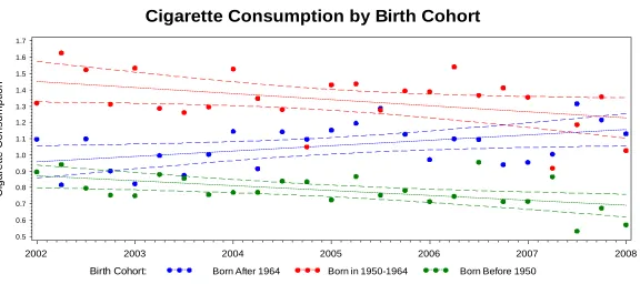
Figure 1.1: 2002-2008 Cigarette Consumption by Birth Cohorts…...………...41
Figure 1.2: 2002-2008 Alcohol Consumption by Birth Cohorts…...………...42
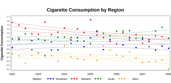
Figure 1.3: 2002-2008 Cigarette Consumption by Region……..…...………...43
Introduction
One can argue that people who consume harmful addictive substances are likely to discount the future more compared to other people. Then, smokers should have present-oriented attitudes in general and are more likely to drink compared to other people. If cigarette consumption affects alcohol consumption (and vice versa), the information about their relationship may allow a better coordination of public policies concerning these two goods. In this dissertation, the relation between cigarette and alcohol consumption is investigated in a rational addiction framework through three essays. Previous studies that estimate cigarette and alcohol demands in the rational addiction framework used aggregate time series data. To analyze addictive behavior, household level data would be a better tool because aggregate data fail to give detailed information about individual behavior. Thus, household level data are used in all three essays in this dissertation.
obtained from Diary data are more reliable for this particular study. Diary data results indicate that cigarette (alcohol) consumption increases the marginal utility from alcohol (cigarette) consumption. On the other hand, long-run cross-price elasticities suggest alcohol is a substitute for cigarettes.
Using Diary data and pseudo-panel approach, the second essay investigates how smoking bans at restaurants affect restaurant alcohol consumption. In the past decade, many U.S. states have imposed smoking bans in a variety of locations. Particularly the smoking bans at restaurants create a natural experiment which allows us to get more insights on the relationship between cigarette and alcohol consumption. An important contribution of this paper is that, while the previous studies analyze how “overall alcohol consumption” is affected by smoking bans, this paper focuses on how “restaurant alcohol consumption” is affected by smoking bans at restaurants. The empirical evidence reveals that smoking bans increase restaurant alcohol consumption. On the other hand, it is found that reductions in the blood alcohol concentration limit for drivers would decrease both alcohol and cigarette consumptions.
Chapter 1
Rational Addiction to Cigarette and Alcohol:
Two Data Sets, Two Different Approaches
1.1.
Introduction
The adverse health effects of smoking and drinking have long been recognized. There are also negative externalities associated with the consumption of cigarettes and alcohol (e.g., health consequences of passive smoking, injuries and fatalities resulting from drunk driving, the effects of alcohol on crime and labor performance). The public health care costs have
made these two goods the prime targets of excise taxation in many countries.
versa), the information about their relationship may allow a better coordination of the public policies concerning these two goods.
The rational addiction model (Becker and Murphy, 1988) is the most popular framework used to estimate the demand for addictive goods like cigarettes and alcohol. Becker and Murphy (1988) claim that addictions to harmful substances are still rational as the decision involves forward-looking maximization of utility. While myopic models of addictive behavior only accounts for addiction, Becker and Murphy’s rational addiction model involves both addiction (i.e., an increase in past consumption increase current consumption), and rationality (i.e., consumer maximizes utility weighting current benefits and future costs). In myopic models, past consumption increases current consumption, but individuals do not take into account the future when making decisions on current consumption. In rational addiction model, the past and the anticipated future consumption both affect current consumption positively.
The rational addiction model has been previously applied to both cigarette consumption (e.g., Chaloupka, 1991; Becker et al., 1994; Jones and Labeaga, 2003) and alcohol consumption (e.g., Grossman et al., 1998; Waters and Sloan, 1995). Bask and Melkersson (2004) extended the rational addiction model to allow for multi-commodity addictions and estimated the demand for cigarettes and alcohol using aggregate time series data.
favor of the rational addiction. They indicate that most of the time time-series data are insufficient to differentiate rational addiction from serial correlation.
In this essay, two different household level data are employed to analyze the relation between cigarette and alcohol consumption in a rational addiction framework. Both data come from Consumer Expenditure Survey (CEX) by U.S. Bureau of Labor Statistics. The Consumer Expenditure Survey (CEX) consists of two separate data sets: a Diary survey and an Interview survey. Each survey uses its own questionnaire and its own sample. In the Interview data, each consumer unit is interviewed once every three months over five consecutive quarters. On the other hand, the sample changes every quarter in the Diary data. Due to the different formats of the two data sets, in order to estimate dynamic demand models, a different methodology is employed for each data set. Within-groups two-step GMM method (Bover and Arellano, 1997) is used for the Interview data. A pseudo-panel data approach is used for the Diary data.
Within-groups two-step GMM method not only deals with censoring, but also allows one to include lags and leads of the dependent variable, other endogenous explanatory variables, and unobserved individual fixed effects in the model. On the other hand, the pseudo-panel approach not only enables one to estimate dynamic demand models using cross-sectional data, but also avoids econometric difficulties due to measurement error, censoring and attrition bias.
1.5 and 1.6 explain the estimation methods used for the Interview and Diary data, respectively. Section 1.7 presents results. Section 1.8 has a discussion of the appropriate data and the methodology. Section 1.9 presents long-run demand elasticities derived from estimation with the Diary data. Section 1.10 concludes the study.
1.2.
Literature Review
Although there is a vast amount of literature on estimating the demand for cigarettes and alcohol separately, there are only a few studies that investigate the interdependence between cigarette and alcohol consumptions. Among these studies only Bask and Melkersson (2004), Fanelli and Mazzocchi (2004) and Pierani and Tiezzi (2009) account for rationality in their specifications. However, all three studies use aggregate time series data in their analyses. Table 1.1 summarizes previous studies on the interaction between cigarette and alcohol consumption.
Goel and Morey (1995) analyze the interdependence between cigarette and liquor demand using a panel of U.S. state level data for the period 1959-1982. Cigarette and liquor demands are estimated separately and the interdependence between two goods is allowed through cross-price effects. The empirical specification accounts for addiction but not rationality. They find a substitution relationship with cross-price elasticities 0.10 and 0.33 for cigarettes and liquor, respectively.
seniors. Cigarette taxes and state minimum legal drinking ages are used to generate full prices of cigarette and alcohol. They find a complementarity relationship between cigarette and alcohol consumption. Elasticities are not calculated. The analysis is static.
Decker and Schwartz (2000) estimate separate static demand equations for cigarettes and alcohol using pooled cross-sectional data from the Behavioral Risk Factor Surveillance System (BRFSS). The interdependence between two goods is allowed through cross-price effects. Their model separates participation from consumption. They find that the cross price elasticity of cigarettes with respect to alcohol price is -0.14, while the cross price elasticity of alcohol with respect to cigarette price is 0.50.
Fanelli and Mazzocchi (2004) analyze the interdependence between tobacco and alcohol demand in UK using aggregate data over the 1963-2003 period. They develop a dynamic Almost Ideal Demand System (AIDS) model which is consistent with the rational addiction theory. They find a complementarity relation between tobacco and alcohol consumption with cross-price elasticities -0.50 and -1.16 for tobacco and alcohol, respectively.
Bask and Melkersson (2004) extend the rational addiction model to include two addictive goods, alcohol and cigarette. They use aggregate annual time series data from Sweden for the period 1955-1999. The sign of the estimated coefficients on lag and lead consumption are consistent with rational addiction theory in alcohol demand equation while it is not the case in cigarette demand equation. Cross-price elasticities are -0.31 and 0.79 for alcohol and cigarettes, respectively.
variation in the data, the demand equations are modeled such that latent consumption
depends on the latent consumption of the other related good. They find a complementarity
relationship between tobacco and alcohol consumption.
Pierani and Tiezzi (2009) employ a rational addiction model to analyze the interdependence between alcohol and tobacco consumption using aggregate annual time series data for the period 1960-2002 in Italy. Cross price elasticities are-0.24 and -1.15 for alcohol and tobacco, respectively.
Yu and Abler (2010) analyze the relation between cigarette and alcohol consumption in rural China, using a panel of provincial data for the period 1994–2003. They find that the cross-price elasticity of cigarette is -0.62, while the cross price elasticity of alcohol is 0.05.
1.3.
Rational Addiction Model
Studies on addictions to harmful substances provide evidence of reinforcement effect. Reinforcement happens when an increase in past consumption increases the marginal utility from current consumption. Since rational consumers consider future negative consequences of harmful behavior, for an increase in consumption to occur the reinforcement effect should be larger.
Following Bask and Melkersson (2004), assume that
where and are quantities of cigarettes and alcohol consumed by consumer i at period t;
and are the habit stocks of cigarettes and alcohol; and is the consumption of a
non-addictive composite good.
The utility function is strictly concave. The marginal utility derived from each good is positive (i.e., , and ; concavity implies , and
). Habit stocks of harmful substances affect current utility negatively due to their
adverse health effects (i.e., and < 0; concavity implies and ). Reinforcement means and . Smoking and drinking are assumed to have
no effect on the marginal utility derived from the composite good (i.e., ). If consumption of alcohol (cigarettes) affects the marginal utility derived
from cigarettes (alcohol) negatively, < 0 and < 0. If consumption of alcohol (cigarettes) reinforces the marginal utility derived from cigarettes (alcohol), and
.
If past alcohol consumption reinforces current cigarette consumption, ; if past cigarette consumption reinforces current alcohol consumption, . Pierani and Tiezzi (2009) call this intertemporal cross-reinforcement effect a quasi-gateway effect. A true
gateway effect refers to the condition where consumption of one addictive substance leads to
later initiation of another addictive substance (Pacula, 1997). When alcohol consumption does not affect the marginal utility from cigarette consumption and vice versa,
The intertemporal budget constraint is
where with rbeing the discount rate, and are prices of cigarettes and alcohol, and is the present value of wealth. As in previous studies, the discount rate is set
equal to the interest rate. The composite good, N, is taken as numeraire, so that , and are expressed relative to the price of the composite good.
The consumer’s problem is:
Following previous studies, it is assumed that and . When the
utility function is quadratic, the first-order conditions from (1.3) generate the following
structural equations for cigarettes and alcohol respectively (see Bask and Melkersson, 2003) :
Economic theory implies with k =1, 2. Rational addiction implies
with .1
If and then alcohol (cigarette) consumption increases the marginal utility from cigarette (alcohol) consumption; and if and then alcohol (cigarette) consumption decreases the marginal utility from cigarette (alcohol) consumption. If past alcohol consumption increases the marginal utility from current cigarette consumption; if past cigarette consumption increases the marginal utility from current alcohol consumption. If there are no quasi-gateway effects across the two goods, .
1.4.
Data
The main data source is the 2002-2008 Consumer Expenditure Survey (CEX) which is conducted by U.S. Bureau of Labor Statistics (BLS). U.S. Census Bureau collects the data for the BLS. BLS use CEX primarily to revise the market basket for the Consumer Price Index (CPI). In the academic literature, CEX data have been used to study many different issues from life-cycle hypothesis to consumer demand (e.g., De Juan and Seater, 1999; Puller and Greening, 1999; Nicol, 2003; Villaverde and Krueger, 2007). The CEX consists of a
1
Diary survey and an Interview survey. Both surveys are conducted at the level of consumer units (CUs)2, but each survey uses its own questionnaire and its own sample.
1.4.1.
Consumer Expenditure Survey (CEX): Interview Component
The Interview component of CEX is a rotating panel. Each household is interviewed every three months over five consecutive quarters. In each quarter, 20 percent of the sample that finished their final interview in the previous quarter is replaced by CUs that are newly initiated. The survey is designed to constitute a representative sample of the U.S. population. Approximately 5,000 households are interviewed in each quarter.
The first interview collects data on the demographic characteristics, which is updated at subsequent interviews. The second through the fifth interviews collect expenditure information from the previous three months. Because the first interview is not reported by BLS, we use the second through the fifth interviews. From now on, the second interview is referred as the first interview, the third interview is referred as the second interview, and so on.
Cigarette, and alcohol expenditures, together with price variables, are used to calculate quarterly consumptions (i.e., cigarette consumption= cigarette expenditure/ cigarette price). The list and definitions of consumer demographics used are given in Table 1.2.
Because CUs are observed only for four quarters, the types of approximating models that can be used are limited. To estimate Equations (1.4) and (1.5), there must be at least four consecutive time period consumption data points for each CU in the survey. The Interview data meets this requirement. Because we need to have the consumption information of each household over at least four consecutive periods, we restrict our sample to CUs with complete interviews for four time periods. Because state information is used to match CUs with state level cigarette prices, we also drop the observations with missing state variables. The very few CUs who report different demographics (i.e., race, etc) over the four quarters that the expenditures are reported are also dropped.
1.4.2.
Consumer Expenditure Survey (CEX): Diary Component
In the Diary data, the sample changes each quarter. The survey is designed to be a representative sample of the U.S. population. The data contain information on CU demographic characteristics and expenditures. The expenditures in the Diary data are collected from CUs for two consecutive one-week periods. Compared to Interview data, the Diary data supplies more information regarding subcategories of alcoholic beverage expenditures.
different demographics (i.e., race, etc) over the two weeks that the expenditures are reported are also dropped.
1.4.3.
Price Variables
Since price data are not collected by CEX, price variables used in the analysis are gathered from other data sources. All price variables are deflated by the Consumer Price Index (CPI) for all items reported on the BLS webpage.
Annual state level cigarette prices are gathered from the State Tobacco Activities Tracking and Evaluation (STATE) System on the website of Department of Health and Human Services, Centers for Disease Control and Prevention (CDC). Prices are weighted averages for a pack of 20 cigarettes. Prices are inclusive of state-level cigarette excise taxes but are exclusive of local cigarette taxes. We merge CEX data and price data by state id variables.
We don’t have state level or household level prices available for alcoholic beverages. To obtain alcoholic beverages prices, we construct Lewbel (1989) price indices which enable us to have household specific price variation.3 Lewbel price indices are calculated using expenditure shares of each CU for different subcategories of alcoholic beverages, i.e., beer at home, wine at restaurant, etc4.
3
Hoderlein and Mihaleva (2008) show that Lewbel price indices produce better empirical results compared to the results obtained using traditional aggregate price indices.
4
1.5.
Methodology for Interview Data:
Within-groups two-step GMM by Bover and Arellano
For the individual level data, consumption variables could be subject to censoring due to abstentions and corner solutions. In that case, the actual consumption of cigarettes ( ) and alcoholic beverages ( ) would be replaced by latent variables, and respectively, in the equations. By using latent variables, it would be possible to capture probability effects (see Labeaga, 1999, for the discussion of the issue in a case study for tobacco consumption). To link observed and latent consumption, we assume a tobit-type observability rule:
(1.6)
We generalize equations (1.4) and (1.5):
7)
(1.8)
where and are latent dependent variables that are not directly observed. T is small and N tends to infinity.5
5
To deal with censoring, dynamics, endogeneous explanatory variables and unobservable fixed effects, we use within-groups two-step GMM method suggested by Bover and Arellano (1997). Because fixed effects are potentially correlated with exogenous variables, we follow Chamberlain (1984) and, Bover and Arellano(1997) in assuming:
k=1, 2 (1.9)
where are all exogenous variables including the real price of cigarettes and alcoholic beverages. contains non-linear terms and/or interactions in .
Following Jones and Labeaga(2003), we also assume:
and (1.10) and
where …., .
Therefore the reduced-form of the model is given by;
(1.11)
Following Bover and Arellano (1997), at the first-stage, we estimate each of the 2xT cross section equations in (1.11) using the tobit model. At the second stage, we apply within-groups method to the model (i.e, equations 1.7 and 1.8) after replacing the latent variables by their predicted counterparts estimated from reduced-form coefficients. The within-groups two-step estimators ( for cigarettes and alcohol are:
(1.12)
with .
.
is the lagged operator, is the lead operator, , K is the
first-difference or within groups operator.
Because Interview data are a rotating panel, following the suggestion of Manuel Arellano, we estimate the first-stage coefficients separately for each group (i.e., a group corresponds to the set of CUs that report consumption over the same time period). In the first-stage, we include demographics, all period prices and interactions between real income and prices. Since we have only 4 time periods, at the second stage we calculate two-step within-groups estimator by applying ordinary least squares (OLS) on fitted first differences. Bootstrapped standard errors are calculated with 1000 replications.
The first-stage estimation of the model requires sufficient price variation over time (i.e., price variation over the four quarters in which consumption is reported by each CU). Thus, to add quarterly price variation to the annual cigarette prices, we employ Litterman’s minimum sum of squared residuals (min SSR) method using state cigarette excise taxes as related series.6 The information on cigarette state excise taxes is reported quarterly on the website of CDC.
6
1.6.
Methodology for Diary Data:
Pseudo-panel Approach
Although individual level panel data have many advantages compared to aggregate data, they generally span short time periods, suffer from measurement error and are subject to attrition bias. In order to avoid these problems, Deaton (1985) suggested using pseudo-panel data approach as an alternative method for estimating individual behavior models.
In the literature, for estimating dynamic models of demand, the pseudo-panel method is a relatively new econometric method. It is an instrumental variables approach in which cohort dummies are used as instruments in the first-stage (i.e., the first stage predicted values are equivalent to cohort averages). The pseudo-panel approach enables one to follow cohorts of people through repeated cross-sectional surveys. Because repeated cross-sectional surveys are often over longer time-periods than true panels, with pseudo panel method models can be estimated over longer time periods. Moreover, averaging within cohorts removes individual-level measurement error (see Antman and McKenzie, 2007).
cause inefficiency. Thus, the challenge when we construct a pseudo-panel is finding a balance between the number of cohorts and the number of individuals within cohorts. The optimal choice would be the one that minimizes the heterogeneity within each cohort but maximizes the heterogeneity among them. In that case, pseudo-panel method results in consistent and efficient estimators.
In most of the applied pseudo-panel studies, the sample is divided into a small number of cohorts with a large number of observations in each (e.g., Browning et al., 1985; Blundell, Browning and Meghir 1994; Propper, Rees and Green 2001). Verbeek and Nijman (1992) showed that if cohorts contain at least 100 individuals and there is sufficient time variation in the cohort means, the bias due to measurement error would be small and can be ignored7.
In the pseudo-panel approach, cohorts can be constructed based on a single characteristic (i.e., birth cohort) or multiple characteristics (i.e., birth and region; birth and education, birth and gender, etc). In this study, we form pseudo-panels based on household head’s year of birth and the geographic region. Cohorts are defined by the interaction of three generations (born before 1950, born between 1950-1964, born in 1965 or later) and four geographic regions (northeast, midwest, south, west). For example, all household heads born before 1950 that reside in the northeast would form one cohort and all households born before 1950 that reside in the midwest would form another cohort. The resulting pseudo-panel consists of a total of 336 observations over 12 cohorts and 28 quarters. This allocation results in around 100 households per cohort.
7
Because pseudo-panel approach is an instrumental variables (IV) method, standard IV conditions should be satisfied for identification (Verbeek and Vella, 2005). The time-invariant instruments should have correlation not only with the lagged and lead consumption variables but also with the exogenous variables in the model (i.e., sufficient cohort-specific variation should be present in the exogenous variables). When we construct our cohorts, we take into account standard instrumental variables (IV) conditions. To have (time-variant) correlation between the model variables and the time invariant instruments (i.e., cohort dummies), we construct our cohorts based on household head’s year of birth and the geographic region. The three generations (born before 1950, born between 1950-1964, born in 1965 or later) are likely to have different consumption patterns which are subject to change over time as the generations age. Different generations are likely to differ also in terms of consumer demographics (e.g., preference for small versus large families) which can change as generations age (e.g., family size changes as children leave the house to start their own family). There are also differences across regions in terms of prices, consumer demographics, and consumption patterns which would change over time because of migration, local policy changes, etc.
among the people born between 1950-1964, which slightly decreases over the sample period. The people born after 1964 have a lower cigarette consumption compared to people born in 1950-1964. This can be explained by the 1964 surgeon general’s report on smoking. The 1964 surgeon general’s report caused awareness about the health consequences of smoking
and changed public attitudes towards smoking.
Figure 1.2 shows alcohol consumption by birth cohorts over the sample period. From 2002 to 2008, the average alcohol consumption slightly increases for all birth cohorts. The oldest birth cohort (i.e., born before 1950) has the lowest alcohol consumption on average.
Figure 1.3 and Figure 1.4 show average consumptions by region. The midwest has the highest cigarette consumption, while west has the lowest. Cigarette consumption decreases in the midwest and west, while it increases in the south and northeast. Over the sample period alcohol consumption slightly increases across all regions, and among all regions the south has the lowest alcohol consumption.
In section 1.3, we derived the structural equations of the following form:
In order the estimate the individual level structural equations (1.4) - (1.5), we use cohort dummies as instruments in the first-stage. Taking cohort averages of (1.4) - (1.5), over
In repeated cross-sectional data, different individuals are observed at each time period. Thus, the lagged and lead variables are not observed for the same individuals in cohort c at time t. Therefore, following the previous literature, we replace these sample means of the unobserved variables with the sample means of the individuals at time t−1, and t+1, respectively, which leads to the following equations8:
where is the average of the fixed effects for those individuals in cohort c at time t.
Since the sample is collected separately at different time periods, is not constant over
time. can be treated as unobserved cohort fixed effect ( ) if there is sufficient number of observations per cohort (see Verbeek and Nijman, 1992). In that case we can estimate the structural equations at the cohort level by using cohort dummies or cohort fixed effects. In the dynamic pseudo-panel data model, the fixed effects estimator on cohort averages is
consistent when T is small and provided that there are no cohort and time effects in the individual error terms once controlled by cohort fixed effects (McKenzie, 2004). The number of observations in each cohort is sufficiently large in our sample to ensure consistency. Thus the fixed effects estimator on cohort averages is calculated.
In the sample, the number of households in each cohort and time period is not the same which might induce heteroskedasticity. Following Dargay (2007), to correct for heteroskedasticity, all cohort variables are weighted by the square root of the number of households in each cohort. To obtain consistent standard errors, bootstrapped standard errors are calculated (1000 replications).
1.7.
Empirical Results
coefficients on lag and lead coefficient are still negative. In the cigarette consumption equation, the coefficient on lag consumption is positive, and the coefficient on lead consumption is negative but none of the coefficients are statistically significant. The coefficient of determination is very low for both cigarette and alcohol equations when 2SLS method is employed (0.06 and 0.04 for cigarettes and alcohol equations, respectively). We drop out the CUs who do not report any cigarette or alcohol consumption and replicate the 2SLS estimation on first differenced equations, and there is no change in the signs of the model coefficients and there is no improvement on the coefficient of determination.
Although the coefficient estimates from 2SLS and within groups two-step GMM methods suggest positive reinforcement between cigarette and alcohol consumptions (i.e., in most specifications, the coefficient on current cigarette consumption in alcohol equation is positive and significant; the coefficient on current alcohol consumption in cigarette equation is positive and significant), one should be cautious in reaching any conclusions based on this analysis since the signs on lagged and lead consumption coefficients are not consistent with the rational addiction model. We also tried different set of demographics/instruments, but there was still no improvement on the estimates.
consumption coefficients are negative which might be due to inventory effects as we derive consumption from expenditures. In the alcohol equation, current cigarette consumption has a positive and significant coefficient which suggests cigarette consumption reinforces alcohol consumption. In the cigarette equation, current alcohol consumption has a positive coefficient which suggests alcohol consumption reinforces cigarette consumption. We have not found any support for quasi-gateway effect across cigarette and alcohol consumption. Lagged cigarette (alcohol) consumption in the alcohol (cigarette) equation is not statistically significant.
Regarding consumer demographics, it is found that as family size increases real expenditures of both cigarettes and alcohol increase. Our results suggest that whites smoke and drink more compared to other races. The consumer units whose household head has a college degree (i.e., associate’s degree or higher) smoke less cigarettes, but drink more alcohol compared to other consumer units. The effect of education on consumption is not statistically significant. Cohort fixed effects are jointly significant in both equations (i.e., the F-test is at the 1% level where F-values are 7.07 and 3.58 in cigarette and alcohol equations, respectively).
1.8.
Discussion
In the Frequently Asked Questions, BLS explains the purpose of Diary and Interview Data:
“The two survey components—the Interview Survey and the Diary Survey—are
designed to collect different types of expenditures. The Interview Survey is
designed to obtain data on the types of expenditures respondents can recall for a
period of 3 months or longer. These include relatively large expenditures, such as
those for property, automobiles, and major durable goods, and those that occur
on a regular basis, such as rent or utilities. Each consumer unit is interviewed
once per quarter for five consecutive quarters. The Diary Survey is designed to
obtain data on frequently purchased smaller items, including food and beverages,
both at home and in food establishments, housekeeping supplies, tobacco,
nonprescription drugs, and personal care products and services. Each consumer
unit records its expenditures in a diary for two consecutive 1-week periods.
Respondents are less likely to recall such purchases over longer periods.
Although the diary was designed to collect information on expenditures that could
not be easily recalled over time, respondents are asked to report all expenses
(except overnight travel) that the consumer unit incurs during the survey week.”
(http://www.bls.gov/cex/csxfaqs.htm).
have been distorted because of the recall error. Recall error has two main forms: omission and telescoping. Omission means forgetting an event entirely. Telescoping, on the other hand, means remembering an event but displacing it in time (i.e., recalling an event as having occurred more recently or longer ago than it actually did). Telescoping occurs, when respondents incorrectly include/exclude an event in the queried time period.
Omission causes underreporting, while telescoping may cause under or over-reporting, so the effect of recall error on the estimates of the model is ambiguous. Memory lapses can also cause simplification and/or modification of answers in a socially desirable direction, which can bias results by suggesting false associations or failing to indicate true relations. It will be particularly problematic if the recall error is systematic (i.e., different type of people have different recall abilities). Gmel and Daeppen (2007) show that recalled alcohol consumption decrease with the length of the recall period (a recall of 7 days versus a recall of 1 day), and recall biases are higher and significant among sporadic drinkers compared to regular drinkers.
1.9.
The Long-Run Elasticities Derived From Diary Data
The results from Diary data are encouraging since the cigarette consumption is consistent with rational addiction theory. To take this one step further, we combine equations (1.4) - (1.5) to obtain a semi-reduced system. As pointed out by Bask and Melkersson (2004), decisions regarding cigarette and alcohol consumption are likely to be determined simultaneously. Thus, although the equations (1.4) - (1.5) give useful information about cross marginal utilities, the true solution of the consumer’s utility maximization problem is:
alcoholic beverage drinkers are social drinkers. The income elasticity is positive and less than one for both cigarettes and alcohol. The cross-price elasticity of cigarette with respect to alcohol price is negative while the cross-price elasticity of alcohol with respect to cigarette price is positive, but only the cross-price elasticity of alcohol is statistically significant.
The results are pretty interesting because long-run price elasticities derived from the semi-reduced system suggest alcohol is a substitute for cigarette while the coefficients of the structural equations suggest that alcohol consumption reinforce cigarette consumption and vice versa. This finding suggests an interesting question: Can two goods be substitutes in prices while they reinforce each other in consumption?
Picone et al.(2004) claim that although alcohol and cigarettes can be complements in
consumption for social drinkers, they are gross substitutes in price. They bring up two
theoretical explanations for the positive cross-price effects: compensation effect, and income
effect. As cigarette prices increase many smokers reduce their consumption or quit smoking.
In that case, smokers substitute alcohol for cigarette as a source of pleasure which is the
compensation effect. In addition, as cigarette expenditures decrease, alcohol consumption
increases due to a positive income effect given that alcohol is a normal good. Decker and Schwartz (2000) come up with a somewhat similar explanation in an analysis of smoking and drinking participation.
plausible to expect that in the face of permanent price increases, smokers would cut their cigarette consumption and reallocate their lifetime income between cigarettes and alcohol. Moreover, rising cigarette prices will give smokers an incentive to decrease consumption or even to quit given that smoking is associated with more serious health problems. As mentioned in Picone et al.(2004) and Decker&Schwartz (2000), people who quit smoking are likely to compensate for the induced stress by increasing alcohol consumption.
1.10.
Concluding Remarks
We use Interview and Diary data by BLS, to analyze the relation between cigarette and alcohol consumption in a rational addiction framework. In the Interview data, each consumer unit reports expenditures for four consecutive quarters. In the Diary data, the sample changes every quarter. Due to the different format of the two data sets, for each data set we employ a different methodology to estimate dynamic demand models. We employ within-groups two-step GMM method suggested by Bover and Arellano (1997) for the Interview data. We employ a pseudo-panel data approach for the Diary data.
The results derived from the Interview data not only contradict rationality but also contradict addictive behavior. The results from the Diary data overall fit better to the rational addiction theory compared to the results from the Interview data.
sub-groups of people have different recall abilities. Because forgetting is unlikely in Diary data, it can be argued that, for the current study, Diary data have more validity than Interview data. Thus, we focus on the estimates from the Diary data.
In the results derived from Diary data, cigarette consumption is consistent with rational addiction whereas alcohol consumption is not (i.e., in the alcohol demand equation lag and lead consumptions have negative coefficients). If there are inventory effects, it might be the reason why we are getting negative coefficients on the lag and lead consumption in the
alcohol demand. The separate demand equations suggest cigarettes and alcohol reinforce each other in consumption (i.e., marginal utility of cigarettes increase as alcohol consumption increases, and vice versa). The cross price elasticity of alcohol with respect to cigarette price which is derived from the semi-reduced system suggests that alcohol is a substitute for cigarettes. Our estimation results are consistent with Picone et al.(2004) who claim that alcohol and cigarettes are gross substitutes in price although they might complement each
other for social drinkers.
Gardes and Starzec (2002) estimate dynamic tobacco and alcohol demands on Polish panel data using an instrumentation based on birth cohorts which is very similar to the pseudo-panel approach that we employ. They compare the pseudo-panel estimation results with the results based on traditional instrumentation methods (i.e., using lag and lead prices as instruments for lag and lead consumption) and find that the pseudo-panel estimates fit the model much better. In the current study, overall pseudo-panel results obtained from using Diary data are also very encouraging. While many applied studies of rational addiction fail to
demand seem plausible. We believe that the pseudo-panel approach has many advantages,
References
Antman, F., and D.J. McKenzie. 2007. "Earnings Mobility and Measurement Error: A Pseudo-Panel Approach," Economic Development and Cultural Change 56: 125-161.
Auld, M.C., and P. Grootendorst. 2004. “An empirical analysis of milk addiction.” Journal of Health Economics 23:1117–1133.
Bask, M., and M. Melkersson. 2003. “Should one use smokeless tobacco in smoking cessation programs? A rational addiction approach.” European Journal of Health
Economics 4:263–270.
Bask, M., and M. Melkersson. 2004. “Rationally Addicted to Drinking and Smoking?”
Applied Economics 36:373-381.
Becker, G.S., and K.M. Murphy. 1988. “A Theory of Rational Addiction.” Journal of
Political Economy 96:675-700.
Becker, G.S., M. Grossman, and K.M. Murphy. 1994. “An Empirical Analysis of Cigarette Addiction.” American Economic Review 84:396–418.
Blundell, R., M. Browning, and C. Meghir. 1994. “Consumer demand and the life-cycle allocation of household expenditure.” Review of EconomicStudies 61: 57–80.
Bover, O., and M. Arellano. 1997. “Estimating Dynamic Limited Dependent Variable
Browning, M., A. Deaton, and M. Irish. 1985, “A profitable approach to labor supply and commodity demands over the life cycle.” Econometrica 53: 503-543.
Chaloupka, F. J. 1991. “Rational Addictive Behavior and Cigarette Smoking.” Journal of
Political Economy 99:722–742.
Chamberlain, G. 1984. “Panel data.” Handbook of Econometrics, vol. 2, Griliches, Z., and
M. Intriligator (eds). North-Holland: Amsterdam.
Dargay, J. 2007. “The effect of prices and income on car travel in the UK.” Transportation
Research Part A 41:949-960.
Deaton, A. 1985. “Panel data from time series of cross-sections.” Journal of Econometrics
30: 109-126.
Decker, S.L., and A.E. Schwartz. 2000. “Cigarettes and Alcohol: Substitutes or Complements?” NBER Working Paper 7535.
Dee, T. 1999. “The Complementarity of Teen Smoking and Drinking.” Journal of Health
Economics 18:769-793.
De Juan., J.P., and J.J. Seater. 1999. “The Permanent Income Hypothesis: Evidence from the Consumer Expenditure Survey.” Journal of Monetary Economics 43:351-376.
Fanelli, L., and M. Mazzocchi. 2004. “Rational Addiction, Cointegration and Tobacco and
Gardes, F., and C. Starzec. 2002. “Evidence on Addiction Effects from Households
Expenditure Surveys: the Case of the Polish Panel.” Econometric Society European Meeting, Venice.
Gmel, G., and J.B. Daeppen. 2007. “Recall bias for seven-day recall measurement of alcohol consumption among emergency department patients: implications for case-crossover designs.” Journal of Studies on Alcohol and Drugs 68:303-310.
Goel, R.K., and M.J. Morey. 1995. “The Interdependence of Cigarette and Liquor Demand.” Southern Economic Journal 62: 451-459.
Grossman, M., F.J. Chaloupka, and I. Sirtalan. 1998. “An Empirical Analysis of Alcohol Addiction: Results from the Monitoring the Future Panels.” Economic Inquiry 36:39–48.
Hoderlein, S., and S. Mihaleva. 2008. “Increasing the price variation in a repeated cross section.” Journal of Econometrics 147:316-325.
Jones, A.M., and J.M. Labeaga. 2003. “Individual Heterogeneity and Censoring in Panel
Data Estimates of Tobacco Expenditure.” Journal of Applied Econometrics18:157–177.
Labeaga, J.M. 1999. “A double-hurdle rational addiction model with heterogeneity: estimating the demand for tobacco.” Journal of Econometrics 93: 49–72.
Litterman, R.B.1983. "A Random Walk, Markov Model for the distribution of Time Series.”
Journal of Business and Statistic, 1:169-173.
McKenzie, D. J. 2004. “Asymptotic theory for heterogeneous dynamic pseudo-panels.”
Journal of Econometrics 120: 235-262.
Nicol, C.J. 2003. “Elasticities of demand for gasoline in Canada and the United States.”
Energy Economics 25:201–214.
Pacula, R. L. 1997. “Economic modeling of the gateway effect.” Health Economics 6:521-524.
Picone, G.A., F. Sloan, and J.G. Trogdon. 2004. “The effect of the tobacco settlement and smoking bans on alcohol consumption.” Health Economics 13:1063-1080.
Pierani, P., and S. Tiezzi. 2009. “Addiction and interaction between alcohol and tobacco consumption.” Empirical Economics 37:1-23.
Propper, C., H. Rees, and K. Green. 2001. “The Demand for Private Medical Insurance in the UK: A Cohort Analysis.” The Economic Journal 111:180-200.
Puller, S.L., and L.A. Greening. 1999. “Household Adjustment to Gasoline Price Change: an Analysis Using 9 Years of US Survey Data.” Energy Economics 21:37-52.
Tauchmann, H., S. Göhlmann, T. Requate, and C.M. Schmidt. 2006. “Tobacco and Alcohol:
Verbeek, M., and T. Nijman. 1992. “Can cohort data be treated as genuine panel data?”
Empirical Economics 17: 9–23.
Verbeek, M., and F. Vella. 2005. “Estimating Dynamic Models from Repeated Cross-Sections.” Journal of Econometrics 127: 83–102.
Villaverde, J.F., and D. Krueger. 2007. “Consumption over the Life-Cycle: Facts from Consumer Expenditure Survey Data.” The Review of Economics and Statistics
89:552-565.
Waters, T.M., and F.A. Sloan. 1995. “Why do People Drink? Tests of the Rational Addiction Model.” Applied Economics 27: 727–736.
Table 1.1. Previous Literature on the Interdependence Between Cigarette and Alcohol Consumption
Papers Data Model Specification εCA εAC
Goel and Morey (1995) panel of U.S. state level data myopic 0.10 0.33
Dee (1999) pooled cross-sectional data static - -
Decker and Schwartz (2000) pooled cross-sectional data static -0.14 0.50 Fanelli and Mazzocchi (2004) aggregate time series rational addiction -0.50 -1.16 Bask and Melkersson (2004) aggregate time series rational addiction 0.79 -0.31
Tauchman et al. (2005) pooled cross-sectional data static - -
Pierani and Tiezzi (2009) aggregate time series rational addiction -1.15 -0.24
Table 1.2. The List and the Definitions of Demographics
Variable Variable Definitions
AGE age of the reference person WHITE 1 if the reference person is white
COLLEGE 1 if the reference person has a bachelor's or a higher degree FAMILY SIZE number of members in CU
Figure 1.1: 2002-2008 Cigarette Consumption by Birth Cohorts C ig a re tt e C o n s u m p tio n 0.5 0.6 0.7 0.8 0.9 1.0 1.1 1.2 1.3 1.4 1.5 1.6 1.7
2002 2003 2004 2005 2006 2007 2008
Cigarette Consumption by Birth Cohort
Birth Cohort: Born After 1964 Born in 1950-1964 Born Before 1950
Regression Equation:
Figure 1.2: 2002-2008 Alcohol Consumption by Birth Cohorts
A
lc
o
h
o
l
C
o
n
s
u
m
p
ti
o
n
10 20 30 40 50
2002 2003 2004 2005 2006 2007 2008
Alcohol Consumption by Birth Cohort
Birth Cohort: Born After 1964 Born in 1950-1964 Born Before 1950
Regression Equation:
Figure 1.3: 2002-2008 Cigarette Consumption by Region
C ig a re tt e C o n s u m p ti o n 0.4 0.5 0.6 0.7 0.8 0.9 1.0 1.1 1.2 1.3 1.4 1.5 1.6 1.7
2002 2003 2004 2005 2006 2007 2008
Cigarette Consumption by Region
Region: Northeast Midwest South West Regression Equation:
Figure 1.4: 2002-2008 Alcohol Consumption by Region A lc o h o l C o n s u m p ti o n 10 20 30 40 50
2002 2003 2004 2005 2006 2007 2008
Alcohol Consumption by Region
Region: Northeast Midwest South West
Regression Equation:
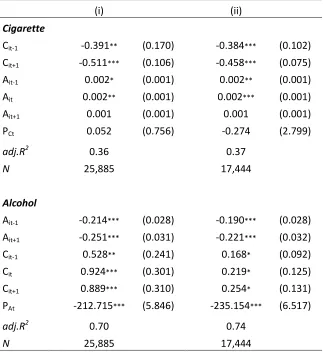
Table 1.3 . Cigarette and Alcohol Demands Estimated Separately Interview Data: Within-groups Two-step GMM Method
(i) (ii)
Cigarette
Cit-1 -0.391** (0.170) -0.384*** (0.102)
Cit+1 -0.511*** (0.106) -0.458*** (0.075)
Ait-1 0.002* (0.001) 0.002** (0.001)
Ait 0.002** (0.001) 0.002*** (0.001)
Ait+1 0.001 (0.001) 0.001 (0.001)
PCt 0.052 (0.756) -0.274 (2.799)
adj.R2 0.36 0.37
N 25,885 17,444
Alcohol
Ait-1 -0.214*** (0.028) -0.190*** (0.028)
Ait+1 -0.251*** (0.031) -0.221*** (0.032)
Cit-1 0.528** (0.241) 0.168* (0.092)
Cit 0.924*** (0.301) 0.219* (0.125)
Cit+1 0.889*** (0.310) 0.254* (0.131)
PAt -212.715*** (5.846) -235.154*** (6.517)
adj.R2 0.70 0.74
N 25,885 17,444
Table 1.4. Cigarette and Alcohol Demands Estimated Separately Interview Data: 2SLS in First Differences
(i) (ii)
Cigarette
Δ Cit-1 0.127 (0.142) 0.140 (0.146)
Δ Cit+1 -0.405 (0.262) -0.521** (0.252)
Δ Ait-1 0.005 (0.005) 0.004 (0.006)
Δ Ait 0.019*** (0.005) 0.019*** (0.006)
Δ Ait+1 0.010 (0.007) 0.012 (0.008)
Δ pCt -6.995* (3.722) -9.870* (5.613)
adj.R2 0.06 0.04
N 25,885 17,444
Alcohol
Δ Ait-1 -0.008 (0.026) -0.002 (0.029)
Δ Ait+1 -0.025 (0.041) -0.028 (0.045)
Δ Cit-1 0.672 (0.720) 0.526 (0.725)
Δ Cit 1.942 (1.768) 1.689 (1.690)
Δ Cit+1 1.610 (1.559) 1.717 (1.597)
Δ pAt -201.788*** (8.712) -202.708*** (9.133)
adj.R2 0.04 0.04
N 25,885 17,444
Table 1.5: Cigarette and Alcohol Demands Estimated Separately Diary Data: Pseudo-panel Method
Cigarette Alcohol
Constant -6.951*** ( 2.086) Constant 162.974*** (55.713)
Ct-1 0.113** (0.048) At-1 -0.085** (0.043)
Ct+1 0.105** (0.051) At+1 -0.106*** (0.039)
At-1 -0.001 (0.002) Ct-1 0.189 (1.103)
At 0.004* (0.002) Ct 2.425** (1.158)
At+1 0.003 (0.002) Ct+1 0.236 (1.009)
PCt -0.060 (0.088) PAt -61.703*** (7.109)
I 0.0001 (0.002) I 0.268*** (0.039)
family size 0.327*** (0.087) family size 6.867*** (1.881)
white 0.768** (0.352) white 37.535*** (7.383)
college -0.338 (0.324) college 7.996 (7.435)
adj.R2 0.67 adj.R2 0.52
Table 1.6. Long-run Elasticities:
Separate Demand Equations
εCC -0.287 (0.371)
εAA -1.339*** (0.201)
εCA -0.323** (0.156)
εAC -0.025 (0.042)
εCI 0.095 (0.080)
εAI 0.409*** (0.056)
Table 1.7: Cigarette and Alcohol Demands Estimated as a Semi-reduced System Diary Data: Pseudo-panel Method
Cigarette Alcohol
Constant -6.546*** ( 2.101) Constant 85.152 (58.083)
Ct-1 0.120** (0.049) At-1 -0.082** (0.043)
Ct+1 0.107** (0.051) At+1 -0.097** (0.038)
At-1 0.0004 (0.002) Ct-1 0.953 (1.092)
At+1 0.002 (0.002) Ct+1 0.725 (0.997)
PCt -0.085 (0.102) PAt -74.066*** (8.282)
PAt 0.099 (0.363) PCt 6.878*** (2.251)
I 0.0001 (0.002) I 0.267*** (0.038)
family size 0.344*** (0.088) family size 5.659*** (1.921)
white 0.793** (0.360) white 29.419*** (7.889)
college -0.314 (0.323) college 6.146 (7.179)
adj.R2 0.67 adj.R2 0.53
Table 1.8: Long-run Elasticities: Semi-reduced System
εCC -0.337 (0.441)
εAA -1.591*** (0.240)
εCA -0.045 (0.324)
εAC 0.777*** (0.295)
εCI 0.089 (0.080)
εAI 0.408*** (0.056)
Chapter 2
How do Smoking Bans Affect Restaurant
Alcohol Consumption?
2.1. Introduction
On November 23, 1998 US state attorneys general signed a tobacco settlement with the five largest tobacco manufacturers. Since then many US states have also imposed smoking bans in a variety of locations (e.g., restaurants, schools, work places). As more cities and states consider smoking bans, it becomes necessary to analyze the economic impacts of these smoking bans.
alcohol consumption. Although there is a vast literature investigating the impact of smoking bans on cigarette consumption, there are only a few studies that analyze the impact of smoking bans on alcohol consumption.
Picone et al. (2004) examine how smoking bans and cigarette prices affect alcohol consumption within a dynamic framework. To account for the addictive nature of these two goods, they add past consumption to the regression models. They find that smoking bans reduce alcohol consumption, but increases in cigarette prices increase alcohol consumption. On the other hand, Gallet and Eastman (2007), using a static model to examine the effects of smoking bans on the state-level demand for beer, wine, and spirits, find that smoking bans at restaurants/bars decrease beer and spirits consumption, but increase wine consumption.
In this study, a rational addiction framework (Becker and Murphy, 1988) is employed to analyze the impact of smoking bans on restaurant alcohol consumption. Consumer Expenditure Survey (CEX), Diary data by U.S. Bureau of Labor Statistics (BLS) is used for the analysis. CEX data are ideal for the purpose of our study as they provide information on alcohol expenditures at restaurants. Thus, rather than analyzing how “overall alcohol consumption” is affected by smoking bans, the focus is given on how “restaurant alcohol consumption” is affected by smoking bans at restaurants. As emphasized by Gallet and
The Diary Data set is composed of repeated cross sections. Thus, in order to estimate the dynamic demand models, a pseudo panel data approach is employed.
The rest of this paper is organized as follows: Section 2.2 summarizes the rational addiction model, section 2.3 gives a discussion of the data set, section 2.4 explains pseudo-panel approach, section 2.5 presents results, section 2.6 explains policy implications, and section 2.7 concludes the study.
2.2. Theoretical Model
Following Bask and Melkersson (2004), we set the consumer’s problem as:
where and are quantities of alcohol and cigarettes consumed by consumer i at period
t; and are the habit stocks of alcohol and cigarettes; and is the consumption of a non-addictive composite good. with r being the discount rate, and are prices of alcohol and cigarettes, and is the present value of wealth. As in previous
studies, we assume that the discount rate is equal to the interest rate. The composite good, N,
is taken as numeraire.