Concurrent Zero Knowledge Proofs with Logarithmic Round-Complexity

Concurrent Zero Knowledge Proofs with Logarithmic

Round-Complexity

Manoj Prabhakaran∗ Princeton University

Amit Sahai† Princeton University

May 6, 2002

Abstract

We consider the problem of constructing Concurrent Zero Knowledge Proofs [6], in which the fasci-nating and useful “zero knowledge” property is guaranteed even in situations where multiple concurrent proof sessions are executed with many colluding dishonest verifiers. Canetti et al. [3] show that black-box concurrent zero knowledge proofs for non-trivial languages requireΩ(log˜ k)rounds wherekis the security parameter. Till now the best known upper bound on the number of rounds for NP languages wasω(log2k), due to Kilian and Petrank [16]. We establish an upper bound ofω(logk)on the num-ber of rounds for NP languages, thereby closing the gap between the upper and lower bounds, up to a ω(log logk)factor.

∗

Email:[email protected].

†

1

Introduction

Zero Knowledge proofs, introduced in [14], are fascinating and important cryptographic primitives. In-formally, a zero knowledge proof is a protocol between a prover and a verifier which yields nothing to the verifier beyond the validity of the assertion proved. However, more recently further refined notions of Zero Knowledge have been introduced to handle scenarios more complicated than the one considered in the original definition.

Zero knowledge proofs in settings involving many asynchronous protocol executions was first consid-ered by Feige [8], who introduced relaxations of the zero knowledge property which were provably pre-served under asynchronous protocol composition. Concurrent Zero Knowledge, introduced in [6], considers a setting in which the prover holds concurrent proof sessions with polynomially many colluding dishonest verifiers.

To show that a protocol is zero knowledge one must show that for every efficient verifier, everything it can do after taking part in the protocol can be simulated by an efficient simulator without taking part in the protocol. Black-box zero knowledge is a restricted version of zero knowledge in which we require that for all verifiers there exist a single simulator which has only black-box or oracle access to the verifier.

Previous Results A large body of fascinating research has dealt with concurrent zero knowledge and related concepts[6, 7, 12, 3, 17, 21, 13, 20, 16, 18, 2, 10, 4, 5, 1]. We review and focus on prior work dealing with black-box concurrent zero knowledge.

It turns out that black-box concurrent zero knowledge is indeed a stronger notion than black-box zero knowledge. Many of the known (black-box) zero knowledge proofs are not black-box concurrent zero knowledge. This is so because lower bounds have been established for the number of rounds in a black-box concurrent zero knowledge proof. Following a sequence of prior work [13, 17, 21], Canetti et al [3] showed that a black-box concurrent zero knowledge proof protocol to prove membership in a language not in BPP requires at least Ω_{log log}logk_k rounds, where k is a security parameter (number of concurrent sessions is polynomial ink).

Subsequently Kilian and Petrank [16], building on the work of [20], showed that under a standard complexity assumption, there exists a black-box concurrent zero knowledge proof system for proving mem-bership in any NP language, with round-complexityω(log2k). There the question was raised whether the same proof system when reduced toω(logk)rounds remains concurrent zero knowledge. In this work we answer that question in the affirmative.

In a recent breakthrough Barak [1] has given the first non-black-box zero-knowledge proof system under standard complexity assumptions. He also presented a (non-black-box) proof system with only a constant number of rounds, which remains zero knowledge for a pre-determined (polynomial ink) number of con-current sessions. The communication in the protocol is proportional to this pre-determined bound on the number of concurrent sessions. Compared to this scheme, our protocol requires ω(logk)rounds, but can handle any polynomial number of concurrent session, and the communication in the protocol is independent of the actual number of sessions.

Our Results We give a black-box concurrent zero knowledge proof for languages in NP, withω(logk)

rounds. This becomes the most efficient concurrent zero knowledge proof system which can handle any polynomial number of concurrent sessions. This round-complexity matches the currently known lower-bound for black-box proofs within a factor ofω(log logk). Also, as in [16] this implies a “resettable zero knowledge proof” system of similar round-complexity.

counting argument, developing a suggestion by Kilian [15], to show that the simulation is indistinguishable from what the verifier sees in the proof. We also provide an alternate description of the simulator introduced in [20], and show that our analysis is asymptotically tight for that simulator.

As described in Section 2 the only quantity to be re-analyzed to establish our improvement is the proba-bility that the simulator aborts in the middle of the simulation. As a warm-up, and as was done in [16, 20] we first analyze the simulator’s abort probability, assuming that the adversarial verifier uses a “static scheduling strategy.” This means that for all points in (protocol) time the verifier has to a priori decide the session from which the message is sent. It cannot adaptively change this schedule during the simulation. But it gets to decide at each point whether the message it sends over is well-formed or not. [16] shows that the probability of the simulator aborting, for the static case is2−Ω(m/logk)_{+(k), for some negligible function}

. We improve on this to establish a probability bound of2−(m−O(logk))_{+(k). Thus with our new analysis,}

choosingm=ω(logk)makes this probability negligible, where as previouslym=ω(log2k)was required. As with [16, 20], our analysis for the static case can be carried over to imply concurrent zero knowledge for general adversaries. Previous analyses of concurrent zero knowledge in the general setting, however, have typically relied on delicate conditioning arguments, notoriously prone to subtle errors.

We develop and present an alternative to the conditioning-based analysis 1 of [20, 16], based on a suggestion to refine the analysis of [20, 16] due to Kilian [15]. The central idea is to essentially prove that for every set of random coins in the simulation which allows the adversary to make the simulator abort, there is a superpolynomially larger set of random coins all of which allow the simulator to succeed without aborting.

We present this argument using an analogy to decks of cards – we view the simulator’s random coins as cards arranged in a sequence (a deck). We show that given any deck which allows the adversary to cause the simulator to abort, we can “shuffle” this deck to produce many new sets of random coins in which the simulator will provably succeed in the simulation without aborting. We then argue that each of the decks produced by our shuffling procedure is unique, by exhibiting a deterministic “unshuffling” procedure that allows us to reconstruct the original deck of cards in which the adversary causes the simulator to abort.

2

Preliminaries

Here we review the basic cryptographic concepts and assumptions we shall need, including black-box con-current zero knowledge, commitment schemes and witness indistinguishability. Note, however, that as we build on the analysis of [20, 16, 18], we will be able to appeal to many of cryptographic arguments of [20, 16, 18] as a black box. Thus, even a reader unfamiliar with the details of cryptographic definitions should be able to follow our analysis.

Formal description and motivation of concepts described below are available in standard references on cryptography, and in particular in Goldreich [11]. [20, 16, 18] have the details and pointers specific to concurrent zero knowledge.

Zero Knowledge Proofs An interactive proof(P, V)for a languageLis a protocol between a computa-tionally unbounded proverP and a probabilistic polynomial time verifierV such that there exists a negligible

1

function(k)such that2for every common inputx(of length polynomial ink) (i) (completeness) ifx∈L

Pr[(P, V)(x)]≥1−(k)and (ii) (soundness) ifx6∈L, for every proverP∗_,Pr[(P∗_{, V)(x)]≤(k).} An interactive proof system is said to be black-box (computational) zero knowledge if there is a prob-abilistic polynomial time oracle machineS such that for any probabilistic polynomial time verifierV∗and for allx∈Lthe distribution of the output produced bySV∗

on inputxis computationally indistinguishable from the view of the verifier at the end of the interaction(P, V)(x).

In concurrent zero knowledge proofs the prover is involved in polynomially many (ink) sessions. We consider the verifiers of all the sessions to be co-ordinated by an adversary. It is up to the adversarial verifier to decide which messages it will send to the prover and when. But the prover should work for each session which behaves correctly as specified by the protocol, irrespective of messages in the other sessions, or their relative order. Proving the concurrent zero knowledge property involves showing that there is a simulator (a probabilistic polynomial time oracle machine) S whose output for everyx ∈ L is computationally indistinguishable from the view of this adversary for thatx.

Commitment Schemes A commitment protocol involves two parties– the sender and the receiver, and two phases– the commit and reveal. In the commit phase the sender commits to a bit (or a string), by sending a commitment to the receiver. But we require the commitment to be secret: it is infeasible for the receiver to find out anything about the committed string. Later in the reveal phase the sender sends over the committed string and possibly more information so that the receiver can verify that the revealed value is identical to the committed value. We require that the commitment is binding on the sender, i.e., it cannot reveal a value other than what it committed to (with overwhelming probability over the randomness chosen by the receiver). This kind of commitment scheme is said to have statistical binding and computational secrecy. The Zero knowledge protocol we analyze will employ such a scheme from [19] in which the receiver initiates the commitment by sending a random string to the sender and the commit phase has a single message from the sender.

The above mentioned commitment is used when the all powerful prover is the sender. We will also need a commitment scheme when the prover is the receiver. For this we require a scheme with information theoretic secrecy and computational binding. [11] describes one, again with a single initiation message from the receiver, a single message from the sender for each commitment, and for each reveal.

Witness Indistinguishable proofs Witness Indistinguishable proofs, introduced in [9], is a notion similar to, but weaker than zero-knowledge. A witness indistinguishable proof for a language in NP is a protocol such that the prover uses some witness to carry out the proof, but the view of the verifier when the prover uses a witnessw1 and that when it uses a different witnessw2 are computationally indistinguishable. This

notion is weak enough to let the security be preserved under concurrent composition.

The concurrent zero-knowledge protocol we are analyzing uses the proof-system for NP languages by Goldreich and Kahan [12]. The proof system involves five messages, the first one from the prover to the verifier. Though the prover is allowed to be computationally unbounded, given a witnesswfor the member-ship of the inputxthe prover can run in polynomial time. This allows us to construct simulators which run in polynomial time, and can carry out the prover’s part in this protocol.

In the concurrent zero knowledge protocol, the witness indistinguishable proof is used with respect to the languageL0 (in NP) defined as follows: (x,preamble) ∈ L0 iff eitherx ∈ L, orpreambleis the transcript of a preamble in which the session was “solved” by the prover (see Section 3 for details). The two witnesses we shall consider forx0 _{∈ L are (i) a witnesswfor x ∈ Lor (ii) a witnessw}0 _forpreamble containing a solution.

Cryptographic Assumptions The cryptographic assumptions we need are the ones on which construc-tions of the above primitives are based. Assuming the existence of a collection of claw-free permutaconstruc-tions suffices for this purpose [11].

Concurrent Sessions In the concurrent setting that we are interested in there are up to`=poly ksessions that run concurrently, using one single prover. In sessionsthe prover is trying to prove that xs ∈ L. The

prover responds to each verifier message in the order in which they come; but it is upto the (adversarial) verifier to choose the session from which the next message sent to the prover comes from.

The simulator and previous analysis We analyze the same protocol as given by [16, 20], except for reducing the number of rounds. The soundness and completeness properties of this system are proved there and the proof holds for the reduced number of rounds too. For proving the zero-knowledge property one needs to demonstrate that for every efficient, but possibly corrupt verifier co-ordinating the verifiers in the polynomially many sessions, there is a simulator such that, for each set of inputs xs, the output of the

simulator and the view of the verifier at the end of the protocol are computationally indistinguishable from each other. [16, 18] gives a black-box simulator, and analyzes the simulator.

They show that to prove this indistinguishability it is enough to show that the probability their simulator aborts in the middle of the simulation is negligible ink.

So we need only analyze the probability that the simulator aborts. We give a better analysis of the same simulator, and show that ifm=ω(logk)the probability of the simulator aborting is negligible.

3

The Protocol

We provide a brief review of the concurrent zero-knowledge proof protocol as described in [16, 18], which in turn is a slight modification of the protocol introduced in [20].

The protocol employs a statistically binding commitment scheme (used by the prover to commit), a statistically hiding commitment scheme (used by the verifier to commit), and a witness indistinguishable proof (interactive proof) system. In Section 2 we briefly reviewed these schemes.

The protocol has two phases– a preamble and a main proof body. The outline of the preamble is provided below:

V →P: Commit tov0, . . . , vm∈ {0,1}k

P→V: Commit top0

V →P: Revealv0

P→V: Commit top1

.. .

V →P: Revealvi

P→V: Commit topi+1

.. .

V →P: Revealvm

P→V: Start the main body of the proof

When the verifier initiates a session, the prover in response initiates the commitment scheme for the verifier. Then the preamble starts, in which the first message from the verifier is a commitment tom+ 1 ran-dom stringsv0, . . . , vm ∈ {0,1}k,kbeing the security parameter (it also initiates the prover’s commitment

scheme). In response the prover commits a random stringp0 ∈ {0,1}k. In subsequent steps, the verifier

revealsvm and the prover starts the witness indistinguishable proof. In all there arem+ 2messages from

the verifier in the preamble.

The witness indistinguishable proof is used with respect to the language L0 (in NP) defined as follows:

(x,preamble)∈L0iff eitherx ∈L, orpreambleis the transcript of a valid preamble such that there is someisuch thatpi =vi.

The protocol continues with the witness indistinguishable proof, in which the prover uses the witness of

x∈L. The verifier accepts or rejects as in that proof system. At any point during the protocol if an invalid message from the verifier arrives, the protocol is terminated.

In the concurrent setting the prover runs the different sessions independent of each other. If a session is terminated further messages from that session are ignored; but it does not affect the other sessions.

We shall show thatm=ω(logk)suffices for the zero-knowledge property of the proof system to hold in the concurrent setting.

4

The Simulator

In this section we describe the simulator of [16], which is based on the simulator of [20]. Our description differs from previously given descriptions, as we identify features of the simulator which we will use to achieve our stronger result.

The simulator does not have access to the witness ofxs ∈ Lfor anyxs. So in the simulated proof it

tries to get a preamblepreamblesuch that(xs,preamble)∈L0, and use information on this preamble

as the witness.

The simulator S has black-box access to the verifier. It randomly sets up the random coins for the verifier in the beginning, and then starts running the verifier and a modified prover on the common inputx. But every now and then the simulator will rewind the verifier. For each sessionShopes to find out the value of some stringvi before committing topi, so that it can commit topi = vi. For thisS should wait till the

verifier reveals somevi and then rewind the execution beyond the point where it committed topi. ButS

cannot afford to do too many rewinds as it must finish running inpoly(k)time.

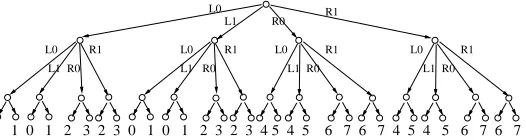
[16] proposes an efficient rewind strategy, which is essentially the same as the rewind strategy of [20]. The rewind strategy is specified with respect to the at mostN := (m+ 2)`preamble messages, numbered from0toN−1. We can assume thatNis a power of two by adding empty “dummy” messages at the end, if necessary. The points0toN−1when a preamble message arrives, are referred to as the protocol points or the protocol time.

Protocol TreeT _{Consider the complete balanced binary tree withNleaves. We shall call this the protocol} tree and denote it byT_{. Height of}T_{ish= logN =O(logk)(as we will consider onlym=O(poly(k))).} It will be convenient later to identify each node inT_{by the path to that node from the root; the path is} specified as a string of L’s and R’s, referred to as the “left-right” or L/R path, in the natural way.

To describe the rewind strategy consider the directed acyclic graph obtained by doubling the edges of T_{except the ones at the leaf level (see figure 1). The schedule is essentially a depth-first traversal of this} DAG, with the slot numbers appearing at the leaves. Informally, the simulator traverses the DAG, and at a node, after returning from the first edge in a double edge, it rewinds the verifier, and continues the traversal by descending the second edge.

L0 L1 R0

R1

0 1 2 3 4 5 6 7 0 1 2 3 4 5 6 7

L0

L0

L1 R0 R1 R1

R0 L1

Figure 1: T_{and the edge-doubled DAG forN = 8}

We separate this string, referred to as the composite path into two strings– the L/R path, and the 0/1 path, in the natural way.

Instances inTˆ _{Each nodeain}T_{has many instances in} Tˆ_{, which are the nodes with the same L/R path as}

ahas inT_{. There is one instance for each 0/1 path. Below, we shall usually denote nodes in}T_{bya, X etc.} and those inTˆ _byˆa,Xˆ _{etc., possibly with some subscripts or superscripts.}

TheN2/2leaves ofTˆ _{correspond to the points at which a preamble message arrives during the} simula-tion. The simulator goes through the leaves of the tree from left to right, and we visualize it as an in-order traversal of ˆT_{. We refer to these N}2_{/2 points in the execution of the simulator as simulation points or} simulation-time (as opposed to protocol-time).

0 1 0 1 2 3 2 3 0 1 0 1 2 3 2 3 4 5 4 5 6 7 6 7 4 5 4 5 6 7 6 7 L0

L1 R0 R1

L0

L1 R0 R1

L0 L1 R0

R1 L0

L1 R0 R1 R0

R1 L1 L0

Figure 2: Simulation treeTˆ_{forN = 8}

Sessions A session during the run of the simulator is identified by the point in simulation time (leaf of

ˆ

T_{) where the first preamble message of the session, namely the initial commit message from the verifier,} arrives. Note that many sessions may simply disappear from the views of the prover and the verifier as the simulator rewinds beyond the start of the session.

The Runs Suppose x is a node inT _{and xˆis an instance of x in} Tˆ_{. The run of x associated with xˆ is} defined as the execution of the simulator from the point at which it traverses down the nodexˆto the point at which it returns fromxˆ. The run ofxˆcan be identified with the interval in simulation-time containing all the descendant-leaves ofxˆ.

Consider a nodexinT_{with childrenyandz. Letxˆbe an instance ofxin}Tˆ_{, with childrenyˆ0,yˆ1,zˆ0and} ˆ

z1. The run ofxatxˆconsists of two runs ofyand two runs ofz. After the first run ofy,yˆ0 the simulator

rewinds – i.e., sets the state of the verifier and the prover to that before the runyˆ0. Then it does another run

ofy,yˆ1. Then it goes on to do two runs ofz, with a rewind between them.

Suppose during the run yˆ0, two properly revealed preamble messagesvi and vi+1 are received from a

rewinds to the state before the start of the runyˆ0. Note that the prover’s messagepi+1is in response tovi,

which has not yet arrived at the point after the rewind. When the simulator continues its run and at some point the reveal ofviarrives, it responds by committing not to a random value aspi+1 but topi+1 := vi+1.

This gives a valid preamble withpi+1 =vi+1which the prover can use as a witness in the main body of the

proof. When the simulator rewinds the runyˆ0, we say that the simulator has solved the sessions.

Once a sessionsis solved as above, the simulator records this in an auxiliary table called the Solution Table. The Solution Table has entries of the form(s, i, vi), for 0 ≤ s < N and0 ≤ i ≤ m. Whenever

the modified prover has to respond with a commitment topi for a sessionsit checks if an entry(s, i, vi)is

available in the Solution Table. If it is, it commits topi=viand notes down this fact and the random coins

used in making the commitment; later when the sessionsenters the main body of the proof the prover can use this information as a witness that(xs,preamble)∈L0without knowing the witness forxs∈L. Since

the main body of the proof is a witness indistinguishable system, using this witness is indistinguishable from what an actual prover will do, and the simulation remains indistinguishable from the real thing.

Note that during the run of the simulator, a sessionsmay reach thei-th message many times; each time the solution from the table (if available) is used to commit topi =vi. Also the session may enter the main

body of the proof many times; again each time a witness will be available from the last commitment ofpi.

Aborting the simulation If at any point in the simulation, a session reaches the main body, i.e., the reveal forvm arrives, and no solution is available for the session, the simulator cannot successfully simulate the

witness indistinguishable proof. If this happens the simulator aborts the entire simulation.

If the simulator does not abort till all the sessions are over (or the verifier terminates), it outputs the view of the verifier at that point. As shown in [20, 16, 18], conditioned on the simulator not aborting, the simulated view it outputs is distributed indistinguishably from the distribution of the view of the verifier after the interaction with an honest prover with witnesses forxs∈Lfor all the sessions.

States of the Simulator We go on to give a more formal description of the simulator in terms of its states during the execution. (This may be skipped without much loss of continuity.)

To describe the rewind schedule formally, we will consider a snapshot of the simulator, when the simu-lator is at a node in its traversal ofTˆ_.3 _{(see below for details). We define the state of the simulator, as this}

snapshot consisting of

(i) The (current) View: The verifier-view consists of a transcript between the prover and the verifier, and the state (work tapes) of the verifier. The simulator also maintains the state of a modified prover (described later). Collectively all this is referred to as the current view.

(ii) Solution Table: the internal table to store the solutions to the solved sessions,

(iii) Book-keeping: A stack of views, called the view-stack, to do the rewinds; a counter to indicate the depth of the current node in the simulation tree Tˆ_{, and a stack of 5-ary values, called the} traversal-stack to traverseTˆ_.

We visualize the operation of the simulator as an in-order traversal of Tˆ_{, as described below. The} simulator starts from the root, traverses down the tree to the left most leaf ofTˆ_{, and waits there for the first} preamble message to arrive; at any time the simulator is at some leaf of Tˆ _{and when a preamble message,} arrives it continues the depth-first traversal until it reaches the next leaf. The preamble message is indexed by the leaf at which the simulator was when the message arrived.

A state describes the simulator at a node inTˆ_{. The top of the traversal stack holds one of the values L0,} L1, R0, R1 indicating the next child to descend into in the traversal, or a special valuereturn. Below we describe the traversal formally by how one state is updated to the next.

Suppose the depth counter indicates that we are not yet at a node just above the leaves. To move to the next state the simulator checks the top of this stack. If the top value of the traversal-stack isreturnit pops the value from the stack and decrements the depth counter. If it is L0 or R0, the current view is saved by pushing it into the view stack, and the top of the traversal-stack is incremented to L1 or R1, resp. Else if the top of the traversal-stack is L1 or R1, the simulator does a rewind by popping the view-stack and replacing the current view with the popped value; also it increments L1 to R0, or R1 toreturn. Finally it moves down in the traversal by incrementing the depth counter and pushing an R0 into the traversal stack, so that the traversal of the child node starts with its first child.

If the depth counter indicates that we are just one level above the leaves, then the simulator has to wait for the next two preamble messages, i.e., it has to move through the two leaves, and then return. For this the simulator keeps modifying the current view by letting the (modified) prover and the verifier run, until two preamble messages arrive. When the second one arrives the simulator moves into the next state by popping the traversal-stack and decrementing the counter.

The Solution Table is a data structure maintained by the simulator and used by the modified prover. While the simulator is running the prover and verifier, the solution table is updated as follows: whenever a properly revealed preamble messagevifrom sessionscomes along, the simulator records the revealed value

as the(s, i)-th entry in the solution table.

Whenever the modified prover has to make the commitment pi for session s, it checks if the(s, i)-th

entry in the table is available. If so it commits that value, marks the session as solved and records the details of this commitment as a solution in the table. If this happens we say the session was solved. Else the prover commits an arbitrary string (say, the zero string).

When the modified prover reaches the main body of proof in a session, instead of entering the witness indistinguishable proof with the witness for the membership ofxs∈L, it looks at the solution table to see

if the session was ever marked as solved. If it was solved, the solution gives a witness in terms of anisuch thatpi =vi, and the modified prover uses this witness. If the session was not solved till this point, then the

prover makes the entire simulation abort.

When all the sessions are over (or the verifier terminates), the simulator outputs the current view of the verifier.

Modified Simulators We use a couple of modified simulatorsS∗ andS†for purposes of analysis. They differ from the original simulator S only in the behaviour of the prover. The simulator S∗ _{has for each} sessions, the witness forxs ∈ L, and its prover uses that for the body of the proof. In S†, in addition to

using these witnesses, the prover always commits to the zero string in the preamble. Though the provers of S∗ _{and S}†_{do not use the entries in the Solution Table, they also abort the simulation if it reaches the} main body of proof in an unsolved session. Note thatS∗andS†are also efficient simulators because in the witness indistinguishable proof system used the prover can run efficiently given a witness forxs∈L.

We would like to show that the distribution of the view output by the simulator S is computationally indistinguishable from that of the view obtained by the verifier as a result of the interaction with the prover. As shown in [16, 20] it is enough to show that the probability that theSaborts is negligible in the security parameterk. The following lets us show this only forS†_.

Proof: This follows from the guarantees of the commitment scheme used by the prover, and the witness indistinguishable proof employed in the main body. S∗ _{serves as a hybrid between S}† _{and the original} simulatorS. The difference in abort probabilities ofS andS∗is negligible by the guarantee on the witness indistinguishable scheme, and that ofS∗ andS†is negligible by the guarantee on the commitment scheme. SandS∗_{are indistinguishable: First we construct hybrid simulatorsS =S}∗

0,S1∗, . . . ,SN∗ =S∗, whereSi∗

uses the witness forxs ∈ Lonly for the sessionss= 0, . . . , i−1. By the hybrid argument it is enough to

show that the abort probabilities ofS∗

i andSi∗+1differ negligibly for alli. We shall construct an adversary

for the witness indistinguishable proof, which has an advantage in distinguishing the witness equal to the difference between the abort probabilities ofS_i∗ andS_i∗₊₁. This is achieved by introducing the proof to be identified into the simulator’s prover for sessioni+ 1. More formally, the adversary is a modification ofS∗

i.

It outputs 1 if the (modified) simulator aborts, and 0 otherwise. The adversary startsS∗

i and if a session gets

started at the simulation pointi+ 1, then it engages with the given prover as follows: when the simulator reaches the main body of proof in sessioni+ 1(if it does at all), the messages from the verifier are directed to the prover. The prover enters the proof with one of the two witnesses– the witness forxi+1 ∈ Lor the

witness in terms of the preamble. If it uses the former, the execution of the adversary is identical to that of S_i∗₊₁ and else to that ofS_i∗. Thus the difference in the abort probabilities ofS_i∗and S_i∗₊₁translates into an advantage in distinguishing the witnesses.

S∗ and S† are indistinguishable: This can be shown in a fashion similar to the above. But this time we are attacking the commitment scheme. The simulator’s prover makes many commitments for each session. So this time we introduce one more level of hybrids to take care of this. DefineS_i,j† as a simulator which

commits to the zero string in all sessions s ≤ ifor the first j commitments. ThenS∗ _{= S}†

0,0 and S† =

S_N,m† ₊₁. Rest of the argument is standard.

In the rest of the paper we analyze the simulatorS†_.

Adversary’s success on (start,stop) The adversarial verifier is said to succeed for a pair of simulation points(start,stop), if the session starting at start point reaches the main proof body at the point stop without S†having solved the session, thereby forcingS†to abort at that point.

Note that for the session to be alive at the point stop, the point start is never rewound beyond, within the interval (start,stop). Formally this means that the current view when the simulator reaches the stop leaf, is obtained by letting the prover and verifier run on the view at the start leaf.

There are onlyO(N2_{) (start,stop)pairs, which is polynomial ink. We shall show that for any given pair}

the probability that the adversary succeeds with respect to that pair is negligible ink. Then the probability of the adversary succeeding is negligible by union bound.

The points corresponding to start and stop in the protocol-time are called proto-start and proto-stop.

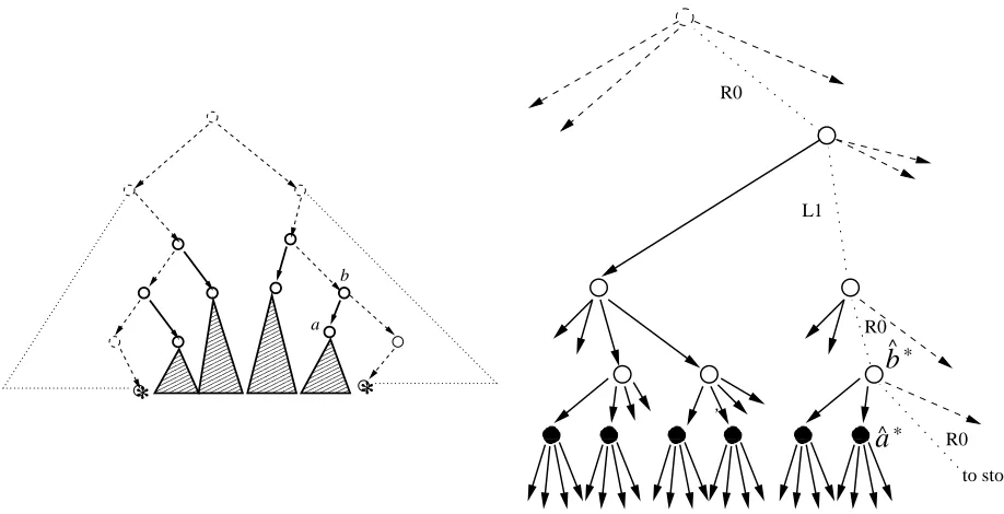
The forests We define a few structures which we shall be referring to frequently throughout the rest of the paper. The protocol forestF_{and the simulation forest}Fˆ _{are subgraphs of}T_andTˆ_{respectively, and are} determined by the pair (start,stop). Later on we also define the good forestGwhich is a subgraph ofF_and is determined by a set ofmprotocol points.

Figures 4 and 4 illustrate these structures.

*

*

a

’ *

b

Figure 3: Left, the Protocol forestF_{as a subgraph of}T_{: the elements in thick outline are part of}F_{. The *’s} indicate the points proto-start and proto-stop. Also, nodeais labeled. Right, a portion of the corresponding Simulation forest Fˆ_{: the 0/1 path of the point stop begins as 0100..; the corresponding composite path is} labeled. This path along with the corresponding path to the start point cut out Fˆ _{from the tree}Tˆ_{. Filled} nodes are all the instances of the nodea. The final instances of nodesaand binF_{are marked in} Fˆ _asˆa∗ andˆb∗_.

Xa

a

t a

2. The simulation forest An edge inTˆ _{is retained in}Fˆ _{if it points to a node all of whose descendant} leaves occur strictly within the simulation interval (start,stop). Fˆ _{is the subgraph of} Tˆ _{induced by} these edges.

We shall focus on these forestsFˆ _andF_{rather than the entire trees}Tˆ_andT_{. Figure 4 illustrates portions} ofF_andFˆ_{, for a given (start,stop) pair. Note that all nodes except possibly the roots of the trees in}F_has all its descendant leaves strictly in the interval (start,stop). If a node ainF_{is at depthd in its tree in the} forestF_{,ahas at least2}d_{instances in}Fˆ_{. (The precise number of instances in}Fˆ _{of a node at depthdin}F_{, is} 2d×(number of instances inFˆ _{of the root of that node’s tree in}F_{).) However}Fˆ _{can have nodes which are} instances of nodes inT_outsideF_.

Now suppose we are given a run ofS†in which the adversary succeeds. Then the (current) transcript when the simulator reaches the point stop will showmpreamble messages of the session, where the verifier properly revealsv0, . . . , vm−1, at somem points in the interval (proto-start,proto-stop). We call these m

protocol points the schedule points of the session. Given such a transcript withmschedule points, we define the following forest:

3. The Good Forest G is the subgraph of F _{induced by all the nodes in} F _{which have at least two} schedule points as descendants (see Figure 4).

The leaves of G essentially correspond to the may-solve intervals as defined in [16, 18] (where it is shown that there are Ω(m/h) such leaves, but we will not need this). They cover disjoint intervals in protocol-time. We order these leaves from left to right according to their intervals, in the natural way.

Pivot Xa and ta For each leaf of G a, let the pivot of a, denoted by Xa, be the node in G defined as

follows:Xais the least common ancestor ofawith the previous leaf inG, or if no such node exists, the root

ofa’s tree inG. Definetaas the distance ofatoXa.

Note that P

ata =number of edges in G, where the summation is over all the leaves of G. This is

because each edge inGis counted in theta whenais the first leaf (in the order defined above) among its

descendants.

Lemma 2 Number of edges in the good forestGis at leastm−O(h), wherehis the height of the protocol treeT_.

Then by the above note, we haveP_ata=m−O(h)where the summation is over all the leaves ofG.

Proof: Define the good treeG0 as a subgraph of the protocol treeT_{, of nodes with at least two schedule} points among descendants. Note thatGis a subgraph ofG0 obtained by removing all the edges which are in the path to the leaves proto-start or proto-stop. Now map each schedule point to its closest ancestor inG0_. Then each leaf inG0 has exactly two points mapped to it and each other node inG0 has at most one point mapped to it (or none if it has degree 2 inG0). So there areΘ(m)nodes with something mapped on to it. SoG0 _{has at least that many nodes. In factG}0 _{has at leastm−1nodes. To see this note that the nodes of} G0with one point mapped to it are internal nodes with only one child inG0, and those with two are leaves of G0; if theren1 andn2of them respectively,n1+ 2n2=m. To haven2leaves,G0must have at leastn2−1

internal nodes of out-degree 2; thus in allG0has at leastn1+n2+n2−1 =m−1nodes. ThusG0has at

leastm−2edges.

We make a few definitions regarding the nodes in Fˆ_.

• Final instance: Consider any nodexinG. There are many instances of this node inFˆ _{(and many in} ˆ

T_outsideFˆ_{, which we do not consider} 4_{). These instances can be ordered by the time the simulator} starts their run. We define the final instance ofx to be the last instance in this order within Fˆ_{. We} denote the final instance ofxbyxˆ∗.

• Critical runs: Consider a leaf ofGa, and its pivotXa. There are many instances of Xa inFˆ. Each

run ofXacontains2ta runs ofa. Consider the last such run,Xˆa∗. We define the2ta runs ofainXˆa∗as

the critical runs ofa. Note that, ifbis a leaf ofGbeforea, the critical runs ofaare all after the run

ˆ_b∗_.

• ˆahii_andaˆh∗i_{: The2}ta_{critical instances of a leafainGappearing inF}ˆ_{are numbered from left to right.}

They are denoted byˆahii for0 ≤ i <2ta_{, whereiis at}

a digit binary number. Note thatˆah2

ta_−1i

is the same asˆa∗_{. We denote this byaˆ}h∗i_{to emphasize that this is a critical run.}

5

Analysis: Static Case

In the static case the adversarial verifier schedules the messages from the various sessions at pre-determined slots. The only choice the adversary gets to make is as to whether the message is revealed properly or not. There arempoints in the protocol time interval(proto-start,proto-stop), where the adversary has non-zero probability of ever scheduling a message from the session. These points are called the potential points. Thus if the adversary succeeds in a run, the schedule points of that run are exactly the potential points.

In the static case we consider theGdefined with respect to the potential points as the schedule points.

• Recall that a leaf ofG has two potential points below it. A run of a leaf ofGis good if the transcript at the end of the run has both the potential messages properly revealed. Else it is called bad.

• A leaf ofGais said to be won (by the adversarial verifier) if all the2ta_{critical runs ofaare bad except}

the final one which is good.

• For each leafaof G, we define phaiias the probability that ˆahii is good given thatˆahjifor all j < i

were bad and all previous leaves ofG were won. The probability is taken over the coin-flips of the simulator (which includes the coin-flips of the verifier and the modified prover).

Lemma 3 phaii=pahjifor alli, j,0≤i < j <2ta.

Proof: It is enough to prove this for the case when the binary representation ofiandj have a hamming distance of one. There is some nodeˆbinFˆ _{which is the least common ancestor of the two critical instances} ofa,ˆahiiandaˆhji. Let the children ofˆb,cˆ0andˆc1be the ancestors ofˆahiiandˆahjirespectively, whereˆc0,ˆc1

are either the L0 and L1 children (resp.) ofˆbor the R0 and R1 children (resp.) ofˆb.

Supposephaii6=pahji. Consider a state of the simulator (as defined earlier) at the start of the run ofcˆ0, and

definep0h_aii (respp0h_aji) by modifying the definition ofphaii (respphaji) by further conditioning on that state.

Thenphaii(respphaji) is a convex combination ofp0haii(resp p0haji) defined with respect to the various states.

Then there is one such stateτ, such thatp0h_aiiandp0h_ajidefined with respect toτ differ.

4

Reasoning similarly, there must exist some state τ0 at the start of the run of ˆc1 such that (i) τ0 is an

extension ofτ(because we are now considering events conditioned onτ) and, (ii)p00h_ajidefined by modifying

p0hji

a by further conditioning onτ0, differs fromp0haii.

We note the following regardingτ andτ0:

(i) The view of the verifier is identical in τ andτ0 _{because τ}0 _{is an extension ofτ (by which we mean} that the simulator can reachτ0starting fromτ) and at the point of starting the run ofˆc1the simulator

rewinds the verifier’s view to the point before it started the run ofcˆ0, to get the view inτ.

(ii) They can differ in the solution tables. But note thatS†_{runs independent of the solution table.}

(iii) The depth counter ofτ andτ0are the same. But the stacks inτandτ0are different: view-stack ofτ is a prefix of that ofτ0, and the tree-traversal-stack ofτandτ0differ in the top value. But during the run ofcˆ0 orcˆ1 both are equivalent; that is, if one is replaced by the other, the simulator will still behave

identically. This is because during the run ofˆc0 orˆc1 (or any run for that matter) the simulator does

not make use of the records already in the stacks before the run starts.

Thus we see that the run ofˆc0 starting from the stateτ and the run of ˆc1 starting from the stateτ0 are

identical and this contradicts the two probabilities being different.

This lets us writepaforphaiifor alli.

Bounding the probability

We consider an adversarial verifier. When the simulator runs, if the adversary has to succeed in taking the session started at the point start to the point stop with out the simulator solving the session, each leafainG must be won (recall that it means all the2ta _{runs ofaare bad except the final one which is good). We seek}

to bound the probability of this event by a negligible function.

Theorem 1 (Static Case) Ifm=ω(logk)the probability that at the point stop, the adversary succeeds in a session starting at start, is negligible.

Proof: In the products below,aranges over all the leaves ofG.

Pr[adversary succeeds]≤Pr[ all the critical runs of all the leaves ofGare won ]

=Y a

Pr[all the critical runs ofaare won|

all the critical runs of all the previous leaves ofGare won]

=Y a

2ta₋₂

Y

i=0

Pr[ ˆahiiis bad|ˆahjiis bad for allj < i,

and all the previous leaves ofGare won]

×Pr[last critical run ofais good|ˆahjiis bad for allj < i, and all the previous leaves ofGare won]

=Y a



 2ta₋₂

Y

i=0

(1−ph_aii) 

ph2

ta_−1i

a ≤

Y

a

But for all values ofpain the range[0,1]and allT ≥1we have(1−pa)Tpa≤

T T+1

T 1

T+1 < T1+1.

So(1−pa)2

ta₋₁

pa≤ 1₂ ta

(this is true forta= 0also). Thus,

Pr[adversary succeeds]≤Y a

1/2ta ₌

1 2

_ata

ButP

ata(where the summation is over all the leafs inG) is exactly the number of edges inG, which by

Lemma 2 ism−O(h) =m−O(logk). If we choosem=ω(logk),P

ata=ω(logk)and the probability

of adversary succeeding is bounded by1/2ω(logk), which is negligible.

6

Analysis: General Case

Now we present the analysis for the general case.

Recall that the adversarial verifier is said to succeed on a run ofS†for a(start,stop)pair, if the session starting at the point start reaches the main proof body at the point stop withoutS† having solved it. We would like to bound the probability that the adversary succeeds. We shall bound this probability for each setting of the coin flips of the verifier. Now onwards we assume the coin flips of the verifier to be fixed. Thus we consider the probability with respect to the coin-flips of the simulated prover only.

Cards and Decks To represent the coin-flips of the simulator, we augment the simulation tree Tˆ _by in-stalling long enough random strings at each leaf. The number of random bits needed by the simulator at each leaf is bounded by a polynomial ink, sayp(k), which we let to be the length of the random string at each leaf. Each such random string is called a card, drawn uniformly from a universe of size2p(k)_{. All the}

N cards in the leaves ofTˆ _{will be collectively referred to as a deck. WhenS}†_{is at a leaf it uses the random} string from the card at that leaf to do its commitments and non-preamble proof steps.

Since we have already fixed the coins of the verifier, given a deck the entire execution of the simulator is determined. Now, to bound the probability that the adversary succeeds we have to bound the number of decks for which the adversary succeeds. We shall show that for every deck for which the adversary succeeds, there are many other decks with which the adversary fails (taking care not to double-count the decks).

Good forest, good nodes and pivot-instance The (start,stop) pair defines the protocol forestF_{and the} simulation forestFˆ_{as before, and also fixes the session we will be considering, namely the session with the} initial verifier commitment at the start point. The only variable then is the deck. Given a deck with which the adversary succeeds, we can define the good tree G from the transcript at the stop point, as described earlier.

Further for each leafaof Gwe can define the pivotXa(and its final instance inFˆ,Xˆa∗), the lengthta

and the2ta _{critical runs ofaas described before.}

A node in Fˆ _{is good if its run adds exactly two properly revealed preamble messages of the session} to the transcript, and each of its descendant nodes’ run adds at most one. Note that the good instance is defined with no reference to “potential-points” orG. Given a deck (with which the adversary may or may not succeed), it is possible to check if an instance is good or not.

If the adversary succeeds with a deck, the good instances are exactly the final instances of the leaves of G. Having a good instance which is not final allows the simulator to solve the session.

Define the pivot-instance of a nodeaˆas a nodeXˆaˆinFˆas follows: if the last good node before the start

andaˆ; otherwiseXˆˆais the root of the tree inFˆcontainingˆa. For a deck with which the adversary succeeds,

ifais a leaf ofGand ˆais any critical instance ofainFˆ_{, thenX}ˆ_ˆa∗ is the same as the final instance of the pivot ofa,Xˆ_a∗.

Lemma 4 There exists a procedure with the following behaviour.

Input: A deckD∗such that the adversary succeeds inD∗.

Output: At least2m−O(h)_{distinct decks, such that in all but one of them,S}†_{solves the session. There exists} a procedureUNSHUFFLEsuch that it unshuffles each of these distinct decks back to the original deckD∗.

We shall prove this lemma shortly, but before that note that it achieves our goal.

Theorem 2 The probability that the adversary succeeds for a given (start,stop) pair is at most2−(m−O(h)).

Proof: All the decks are equally probable. Lemma 4 says that for every deck with which the adversary succeeds there are 2m−O(h) _{− 1 other decks for which it doesn’t. Being able to unshuffle these decks}

to the original one guarantees us that we do not double-count any of them for different decks given by the adversary. Thus the existence of a procedure as described in Lemma 4 establishes an upper bound of

2−(m−O(h))on the probability that the adversary succeeds.

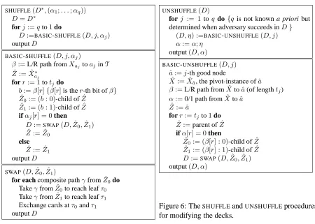
Shuffle-Unshuffle In order to prove Lemma 4, first we give a procedureSHUFFLEand an inverse procedure

UNSHUFFLE.

Let the leaves of G, from left to right, bea1, a2, . . . , aq. The shuffle procedure SHUFFLEconsists of a

sequence of basic shuffles, one associated with each leaf ofG. The leaves are processed right to left, i.e. in the orderaq, . . . , a1.

SHUFFLEtakes a deckD∗in which the adversary succeeds. With this deck there are many good instances as defined above, but all of them have to be final. The aim ofSHUFFLEis to produce a new deck such that

these final good instances get moved around and occur as non-final good instances, allowing the simulator to solve the session.

The algorithm is described in Figure 6. Note that we refer to the L0 child of a node Xˆ in Fˆ _as (L: 0)-child ofX and so on.

SWAPdoes an atomic shuffle operation, exchanging the cards at the leaves of a run Zˆ0with that of a run

ˆ

Z1; informally, this advances the run ofZˆ1 ahead of that ofZˆ0, as the runs of these nodes are essentially

determined by the cards at the leaves. BASIC-SHUFFLE(D, j, α_j)will shuffle the deck so that the final and good run ofαj,ˆah∗ij is advanced to the nodeˆa

hαji

j . Ifαj is the all-ones string this does not change anything;

but otherwiseaˆhαji

j is a non-final run and after the shuffle is a good run, allowing the simulator to solve the

session.

Lemma 5 If the firstjgood instances with the deckDareaˆh∗i₁ , . . . ,ˆa_jh∗i₋₁,ˆah∗i_j , then the deckD0 =BASIC

-SHUFFLE(D, j, α_j) is such that (I) the first j good instances with D0 are ˆah∗i₁ , . . . ,aˆh∗i_j−1,aˆhαji

j , and (II) BASIC-UNSHUFFLE (D0, j)gives(D, αj).

Proof: (I) We examine the steps during the shuffle. Letαj/rdenote the stringαj but with the lasttaj−r

bits replaced by all ones. We shall establish that afterriterations of the loop in BASIC-SHUFFLE, with the resulting deckaˆhαj/ri

j is the j-th good instance; then, since at the end of the subroutine r = taj we have

thatˆahαj/ri

j = ˆa hαji

j is thej-th good instance as claimed. We shall also show that the firstj−1good nodes

SHUFFLE(D∗_{,(α1;. . .;αq))}

D=D∗

forj:=qto1do

D:=BASIC-SHUFFLE(D, j, αj)

outputD

BASIC-SHUFFLE(D, j, αj)

β :=L/R path fromXaj toajinT ˆ

Z := ˆX∗

aj

forr:= 1totjdo

b:=β[r]{β[r]is ther-th bit ofβ} ˆ

Z0:= (b: 0)-child ofZˆ

ˆ

Z1:= (b: 1)-child ofZˆ

ifαj[r] = 0then

D:=SWAP(D,Zˆ0,Zˆ1)

ˆ Z:= ˆZ0

else ˆ Z:= ˆZ1

outputD

SWAP(D,Zˆ0,Zˆ1)

for each composite pathγfromZˆ0do

TakeγfromZˆ0to reach leafτ0

TakeγfromZˆ1to reach leafτ1

Exchange cards atτ0andτ1

outputD

UNSHUFFLE(D)

forj := 1 toq do{q is not known a priori but determined when adversary succeeds inD}

(D, η) :=BASIC-UNSHUFFLE(D, j)

α:=α;η output(D, α)

BASIC-UNSHUFFLE(D, j)

ˆ

a:=j-th good node ˆ

X := ˆXˆa, the pivot-instance ofˆa

β:=L/R path fromXˆtoˆa(of lengthtj)

α:=0/1 path fromXˆtoˆa ˆ

Z:= ˆa

forr:=tjto1do

ˆ

Z:=parent ofZˆ ifα[r] = 0then

ˆ

Z0:= (β[r] : 0)-child ofZˆ

ˆ

Z1:= (β[r] : 1)-child ofZˆ

D:=SWAP(D,Zˆ0,Zˆ1)

output(D, α)

Figure 6: TheSHUFFLEandUNSHUFFLEprocedures for modifying the decks.

We use induction onr. Whenr = 0,αj/0is the all-ones string, andˆahjαj/0i = ˆa h∗i

j . The claim is true

by the assumption on the input. Now we consider r > 0. At the beginning of the r-th iteration Zˆ is at a distancetaj −r+ 1 fromˆa

hαji

j , andˆa hαji

j is under the (β[r] :αj[r])-child ofZˆ. Ifαj[r] = 1, then in

ther-th iteration of the loop inBASIC-SHUFFLEthe deck stays unchanged andαj/r = αj/(r−1); so the

conclusion follows trivially. But if it is 0 a swap takes place, in which the cards on the leaves of the subtree underZˆ1 are moved to the leaves of the subtree underZˆ0. The subtree under Zˆ1containsaˆh_jαj/r−1iwhich

by induction hypothesis, is thej-th good instance before the swap. Also at that point the subtree under Zˆ0

does not have any good instance because thej−1-st good instance isaˆh∗i_j−1which occurs beforeZˆ0.

The simulator has the same state when it starts the run ofZˆ0and the run ofZˆ1 except for the contents

already in its stacks, which are not examined during the runs, and the contents of the Solution Table, which are also ignored by the simulatorS†. The cards at the leaves ofZˆ1 before the swap appear at the leaves of

ˆ

Z0 after the swap. So the run ofZˆ0with the deck after the swap is identical to the run ofZˆ1with the deck

before the swap. (But the execution afterZˆ1may now be totally different from anything before the shuffle.)

Further the cards at the leaves of all the runs completing before the start of the run of Zˆ0 remain

un-changed. Hence with the new deck, the good nodes encountered before starting the run ofZˆ0are exactly the

ones encountered till then with the old deck. Thus after ther-th iteration, ˆahαj/ri

j is thej-th good node for

the new deck and the firstj−1good nodes remain unchanged. (II) By the above, thej-th good node withD0 isˆahαji

j (denoted in BASIC-UNSHUFFLE asaˆ) and the one

before that isˆah∗i_j−1. So the pivot-instance ofˆahαji

j is the same as that ofˆa h∗i

j withD, and is denoted asXˆ.

Then the 0/1 path fromXˆ toˆa(denoted asα) isαj. Alsoβ, the L/R path fromXˆ toaˆis the same as the L/R

done byBASIC-SHUFFLE(note thatSWAPis its own inverse operation).

Proof of Lemma 4: The complete shuffling procedure takes q shuffle-strings α1. . . αq, and the deck

given by the adversary D∗ (such that the only good nodes withDq are theq final instancesaˆh∗i1 . . .ˆa

h∗i q ).

Let Dq := D∗. It then applies the shuffle subroutine repeatedly to produce Dj−1 := BASIC-SHUFFLE (Dj, j, αj), forj=q, . . . ,1. The final deckD0is output.

UNSHUFFLE applies the BASIC-UNSHUFFLE repeatedly to this deck. By the above claim we have

(Dj, αj) :=BASIC-UNSHUFFLE (Dj−1, j), forj = 1,2, . . . , q(q can be found out once it reaches a deck

with which the adversary succeeds). ThusUNSHUFFLEindeed recoversD∗andα1. . . αqfromD0.

αj is ataj long bit string, and therefore there are2 aj

t_aj

strings (α1;. . .;αq). Consider a procedure

which callsSHUFFLEwith all of them. SinceUNSHUFFLEcan recover(α1;. . .;αq)from the shuffled deck,

this way we get2 ajtaj _{distinct decks. But}P

ajtaj is equal to the number of edges inGand by Lemma 2

is at leastm−O(h).

To complete the proof we observe the following: when all theqshuffle-strings are all-ones strings, the resulting deck is the original deck. For any other collection of shuffle-strings, the resulting deck lets the simulator solve the session: suppose αj is the first not-all-ones shuffle-string. Then aˆh_jαji is a non-final

instance which is good. This allowsS†with this deck to solve the session.

In Theorem 2 if we setm=ω(logk), the probability of the simulator aborting becomes negligible (ash

the height of the simulation tree isO(logk)). By the analysis in [16, 18] this establishes that this protocol of round complexity ω(logk)is a concurrent zero knowledge for languages in NP, yielding the improvement that we promised.

7

Tightness of the analysis

Our analysis of the simulator is asymptotically tight. We demonstrate that ifm < h,hbeing the height of the protocol tree, then a simple deterministic schedule by the verifier can make the simulatorS abort with probability one. Note that withΘ(k)sessionsh= Θ(logk). Som =O(logk)rounds is not sufficient for Snot to abort the simulation.

The first preamble message (verifier’s commit) is scheduled at the first protocol point, 0 and the last one in response to which the prover has to enter the main body of the proof is scheduled at the last pointN−1, whereN = 2h_{. The otherm < hpreamble messages are scheduled at theh−1protocol points numbered}

N/2, N/2 +N/4, . . . , N−2. The verifier deterministically reveals all the messages properly.

Then it is not hard to verify that the first time the simulator reaches the pointN−1, the session wouldn’t have been solved.

8

Conclusion

We have shown concurrent zero knowledge proofs for languages in NP with round complexityω(logk). In [3] it is established that if the round-complexity of a concurrent zero-knowledge proof system for a language

Acknowledgments

We gratefully thank Joe Kilian for sharing his thoughts with us and generously giving us his permission to use and build up on his suggestion [15] for a general-case analysis which avoids conditioning. This suggestion came out of discussions between the authors and Kilian regarding the dangers and subtleties involved in conditioning-based analyses.

References

[1] B. Barak. How to Go Beyond the Black-Box Simulation Barrier. In 42nd IEEE Symposium on Foun-dations of Computer Science, pages 106–115, 2001.

[2] R. Canetti, O. Goldreich, S. Goldwasser, and S. Micali. Resettable Zero-Knowledge. (revised version available from http://www.wisdom.weizmann.ac.il/˜oded/p_cggm.html). In ACM Symposium on Theory of Computing, 2000.

[3] R. Canetti, J. Kilian, E. Petrank, and A. Rosen. Black-box Concurrent Zero-Knowledge Requires Omega (log n) Rounds. In ACM Symposium on Theory of Computing, pages 570–579, 2001.

[4] G. D. Crescenzo and R. Ostrovsky. On Concurrent Zero-Knowledge with Pre-processing. In CRYPTO, pages 485–502, 1999.

[5] I. D˚amgard. Efficient Concurrent Zero-Knowledge in the Auxiliary String Model. In EUROCRYPT, 2000.

[6] C. Dwork, M. Naor, and A. Sahai. Concurrent Zero-Knowledge. In ACM Symposium on Theory of Computing, pages 409–418, 1998.

[7] C. Dwork and A. Sahai. Concurrent Zero-Knowledge: Reducing the Need for Timing Constraints. In CRYPTO, pages 442–457, 1998.

[8] U. Feige. PhD thesis, Weizmann Institute of Science, 1990.

[9] U. Feige and A. Shamir. Witness Indistinguishability and Witness Hiding Protocols. In 22nd ACM Symposium on the Theory of Computing, 1990.

[10] O. Goldreich. Concurrent Zero-Knowledge With Timing, Revisited. (available from

http://www.wisdom.weizmann.ac.il/˜oded/p_conc-zk.html), 2001.

[11] O. Goldreich. Foundations of Cryptography – Basic Tools. Cambridge University Press, 2001.

[12] O. Goldreich and A. Kahan. How to Construct Constant-Round Zero-Knowledge Proof Systems for NP. Journal of Cryptology, 9(2):167–189, 1996.

[13] O. Goldreich and H. Krawczyk. On the Composition of Zero-Knowledge Proof Systems. SIAM Journal on Computing, 25(1):169–192, 1996.

[14] S. Goldwasser, S. Micali, and C. Rackoff. The Knowledge Complexity of Interactive Proof-Systems. SIAM Journal on Computing, 18:186–208, 1989.

[16] J. Kilian and E. Petrank. Concurrent and resettable zero-knowledge in poly-logorithmic rounds. In ACM Symposium on Theory of Computing, pages 560–569, 2001.

[17] J. Kilian, E. Petrank, and C. Rackoff. Lower Bounds for Zero Knowledge on the Internet. In IEEE Symposium on Foundations of Computer Science, pages 484–492, 1998.

[18] J. Kilian, E. Petrank, and R. Richardson. Concurrent Zero-Knowledge Proofs for NP. (available athttp://www.cs.technion.ac.il/˜erez/publications.htmlfrom the public web-page of Erez Petrank ), 2001.

[19] M. Naor. Bit Commitment Using Pseudorandomness. Journal of Cryptology: the journal of the International Association for Cryptologic Research, 4(2):151–158, 1991.

[20] R. Richardson and J. Kilian. On the Concurrent Composition of Zero-Knowledge Proofs. In EURO-CRYPT, pages 415–431, 1999.