20th International Conference on Structural Mechanics in Reactor Technology (SMiRT 20) Espoo, Finland, August 9-14, 2009 SMiRT 20-Division 1, Paper 1779
Using Spatial Statistical Analysis of Taylor Factors to Characterize Material
Susceptibility to Intergranular Stress Corrosion Cracking
Mikko I. Jyrkama
a, Mahesh D. Pandey
a, and Edward M. Lehockey
ba
Department of Civil and Environmental Engineering, University of Waterloo, Waterloo, Ontario, Canada e-mail: [email protected]
b
Ontario Power Generation, Pickering, Ontario, Canada
Keywords: Stress corrosion cracking, Taylor factor, Spatial statistics, Variogram.
1
ABSTRACT
Studies have shown that variations in Taylor factor from one grain orientation to the next can help predict failure in materials. The differences in Taylor factor between neighbouring grains increases the likelihood of dislocation pile-ups at the grain boundaries. Sharp dislocation gradients resulting from large contrasts in Taylor factors lead to the formation of voids, which act as a precursor to future intergranular stress corrosion cracking. In this study, the spatial variability in Taylor factor is correlated with failure potential using spatial statistical analysis. The spatial correlation of Taylor factors is quantified through variogram analysis, which describes the dissimilarity in Taylor factor across the sample as a function of lag distance. The methodology is applied to the analysis of cracked and un-cracked samples of carbon steel piping. The Taylor factor mapping was obtained through Orientation Imaging Microscopy (OIM). The results of the study demonstrate how the variogram provides a quantifiable measure of variability that is consistent across samples at different scales, and hence is an effective method for identifying material susceptibility to intergranular cracking.
2
INTRODUCTION
Previous investigations have noted that variations in Taylor factor between adjacent grains can indicate the failure potential in materials (Wright and Field 1998). For example, grains with low Taylor factors next to grains with relatively high Taylor factors are more susceptible to large stress concentrations, and hence intergranular cracking. The susceptibility is manifested as dislocation pile-up at the grain boundaries which increases the probability of intergranular defect nucleation. The distribution of Taylor factors among a large sampling of grains from a particular sample may exhibit a bi-modal shape, thereby resulting in a higher likelihood of encountering adjacent grains having large differences in Taylor factor (Lehockey et al. 2007). While describing the material susceptibility to cracking in a general sense, the sampling distribution provides no information at the local grain scale where the differences in Taylor factor are most critical.
The objective of this study is to correlate the spatial variability in Taylor factor with crack behaviour and failure potential using spatial statistical analysis. The spatial correlation of Taylor factors is quantified through variogram analysis, which describes the dissimilarity in Taylor factor across the sample as a function of lag distance. The lag vector represents the separation between two spatial locations and provides directional dependence (e.g., transverse versus radial direction) for the computed variograms. Therefore, the spatial correlation structure embodied in the variogram describes the variability of Taylor factor not only as a function of scale (i.e., from intra-granular to multiple grain sizes), but also in terms of direction.
3
BACKGROUND
Orientation Imaging Microscopy (OIM) allows the automated collection and indexing of electron backscattered diffraction patterns generated in a scanning electron microscope (Adams et al. 1993; Dingly and Adams 2000). The grain boundary structure is established by measuring the angular misorientations between adjacent lattices/grains, which collectively defines material texture. The Taylor factor, representing a measure of required plastic work (Taylor 1938), can then be calculated for each sample point or grain describing the orientation of slip systems relative to any postulated, user defined, stress tensor.
3.1 Data Sets
Severe degradation of carbon steel piping was a key factor leading to the early refurbishment of a CANDU reactor (Slade and Gendron 2008). Significant inner- and outer-diameter initiated intergranular cracking was found in twelve tight-radius bends of SAE 106B carbon steel feeder piping. The feeder pipes carry the heavy water coolant between the reactor core and the steam generators. While no cracked feeders have been found to date in any of the other operating CANDU stations, there is concern that this degradation mechanism may affect the other units sharing the same pipe material. There is therefore good motivation for trying to identify and characterize the material susceptibility to this type of degradation mechanism.
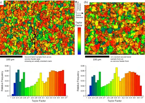
Figure 1a shows the Taylor factor map for a cracked sample from a feeder removed from the refurbished reactor, while Figure 1b illustrates the results from an ex-service un-cracked feeder pipe from another station. Both pipes were manufactured from SAE 106B carbon steel material. The Taylor factors are represented on a colour scale for a postulated hoop stress, where the slip systems that are oriented progressively less favourably to accommodate strains are coloured from blue to red. The OIM sampling interval for the cracked sample was approximately 0.5 µm, while the un-cracked sample was analyzed at a larger 1.0 µm resolution. The samples were obtained from the second bend of each outlet feeder.
Figure 1. Taylor factor maps and distributions for (a) a cracked sample (showing an axially oriented crack in
the middle of the scan) and (b) an un-cracked sample from another station. 100 µm
T
ra
n
s
v
e
rs
e
D
ir
e
c
ti
o
n
Radial Direction
Taylor Factor
100 µm Second bend sample from an
ex-service feeder pipe
showing an axially oriented crack.
Un-cracked second bend sample from an ex-service feeder from another station.
The distributions of Taylor factor for the samples are also shown in Figure 1. As illustrated in Figure 1, the distributions look nearly identical with the cracked sample having a slightly larger proportion of Taylor factor at the low and high ends of the spectrum. While a strongly bi-modal distribution will increase the statistical likelihood of encountering adjacent grains with large differences in Taylor factor, it is difficult to assess the relative susceptibility of the two samples to intergranular cracking based on Figure 1 alone. The distributions from archived and other ex-service feeders from various locations tend to support this observation by exhibiting nearly identical distributions of Taylor factor to the two samples presented here. It is therefore necessary to employ spatial statistical techniques to analyze the spatial variability of Taylor factor within and between these two samples.
4
METHODOLOGY
Spatial correlations of materials, including microstructures, have been analyzed using various methods (Ripley 1977; Spitzig et al. 1985; Stoyan and Wiencek 1991; Pyrz 1994; Vicens et al. 1997). Techniques have also been developed for analyzing the variability in Taylor factor (Yang 1999; Przybyla et al. 2007). The variogram is a spatial analysis technique developed and used extensively in geostatistics to analyze spatial autocorrelation, particularly in mining applications (Matheron 1967; Isaaks and Srivastava 1989; Cressie 1993).
4.1 Variogram Analysis
Consider some variable, e.g. Taylor factor, expressed as a function of spatial location, z(u), where u is the vector of spatial coordinates (e.g., x and y). Note that boldface lettering is used to indicate vector quantities. Because we are interested in the variability of the parameter in space, we consider measurements of the same variable (i.e., data pairs) made some distance apart from each other. Similar to time series analysis, the separation distance is usually referred to as the “lag”. Because of spatial analysis, however, the lag, h, is here defined as a vector. The lagged version of the variable is then denoted as z(u + h).
While covariance and correlation describe the similarity between variables, semi-variance acts as a measure of differences and is defined as (Matheron 1967)
(1)
where N(h) is the number of data pairs represented by the lag h. While equation (1) represents the semi-variance, the variance is given as 2γ (h). Semi-variance (or variance) is therefore simply equivalent to the mean squared difference between the data pairs for a given lag.
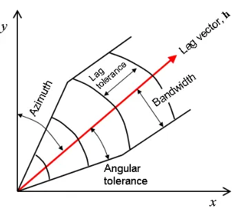
Because the lag vector, h, is a function of both magnitude and direction, the semi-variance is computed spatially across the entire sample. Essentially this involves taking the difference between all data points with each other while keeping track of the lag vector. To ensure sufficient number of points in the estimate, both a distance and an angular tolerance are used to collect the data into groups as illustrated in Figure 2. To avoid bias in the results, statistics should not be calculated for lag distances greater than one-third to one-half of the total sample extent.
4.1.1 Semi-variogram model
The semi-variogram (often simply referred to as the variogram) is based on modelling the squared differences in the z-values as a function of the distances between all the known points. It consists of plotting the calculated semi-variance against the lag distance. The semi-variogram (or variogram) model is shown schematically in Figure 3.
Figure 2. Lag vector tolerances. Figure 3. The semi-variogram model.
The semi-variogram can be computed for the principal data directions (e.g., x and y), or for any arbitrary direction (anisotropic). It is also possible to construct an omni-directional variogram by integrating the semi-variance in all the directions for each lag distance (i.e., removing the angular component of lag by integration).
4.1.2 Variogram map
As opposed to the one-dimensional semi-variogram model, a variogram map allows the visual interpretation of semi-variance in all directions at the same time. It helps to identify appropriate principal axes for defining an anisotropic variogram model. The variogram map is constructed by fitting a surface to the estimated semi-variances based on the directional lag vector (angle and distance). The centre of the map corresponds to the origin of the variogram for every direction, while a transect in any single direction is equivalent to the basic one-dimensional variogram in that direction (e.g., 0° corresponds to the principal x-direction while 90° corresponds to the principal y-direction).
4.2 Variogram Interpretation
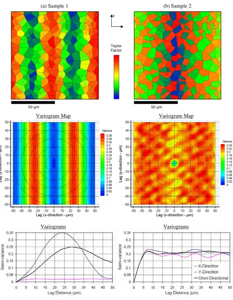
Interpretation of the variograms is illustrated through simulation. Figure 4 shows two simulated samples with a colour scale corresponding to the Taylor factor spectrum presented previously in Figure 1. The corresponding variograms and variogram maps for the samples are also shown in Figure 4. The average grain size for the samples is approximately 8 µm, with the same distribution of Taylor factors (only re-arranged differently among the grains) having a global variance equal to 0.19.
As shown by the variograms and variogram maps in Figure 4, the variability, or difference in Taylor factor is minimal for Sample 1 in the principal y-direction. The difference in the maximum lag in the x -direction is attained at about 24 µm, corresponding to the distance between grains having the maximum difference in Taylor factor (blue vs. red). The results for Sample 2 indicate high variability between neighbouring grain Taylor factors, as evidenced by the “cyclicity” in the variograms and the “patchiness” in the variogram map.
The omni-directional variogram is obtained by integrating around the centroid of the variogram map for each lag distance, i.e., removing (integrating out) the angular component from the lag vector. As shown by Figure 4, the omni-directional variogram tends to lie somewhere in the middle of the two principal direction (i.e., x and y) variograms.
Figure 4. Simulated Taylor factor maps and corresponding variograms and variogram maps for (a) Sample 1
and (b) Sample 2. Both samples have approximately the same Taylor factor distribution.
4.3 Indicators of Cracking Susceptibility
Based on the results of the simulation study, the key factors in the variogram analysis influencing the material susceptibility to cracking are
1. how quickly and how high the variogram rises, and 2. the periodicity and amplitude of the cyclicity.
50 µm
y
x
(a) Sample 1 (b) Sample 2
Variogram Map Variogram Map
Variograms Variograms
50 µm Taylor
The faster and higher the variogram rises, the more the variability in the Taylor factors across the neighbouring grains Similarly, a greater amount of cyclicity indicates the presence of neighbouring grains with contrasting Taylor factors, and hence, higher potential for void formation. A sample with smaller grains would provide a higher number of potential defect nucleation sites (per area). This scale affect due to grain size is also readily captured by the variogram model as reflected in the rise of the variogram.
5
RESULTS AND DISCUSSION
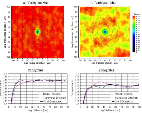
Figure 5 shows the variogram analysis results for the cracked and un-cracked carbon steel feeder pipe samples presented earlier in Figure 1. As shown by the results in Figure 5, the cracked sample (a) shows a significantly higher overall variability in Taylor factor as compared to the un-cracked sample (b). This is evident in both the variogram maps (the colour scales are the same for both samples) and the variograms.
The variogram map for the un-cracked sample (b) also shows an interesting result with respect to texture. The variogram reaches a maximum value at approximately 35 µm in the transverse direction, with a repeating pattern, while the variability is less in the radial direction. This implies that on average, there are bands of grains with opposing Taylor factors separated by 35 µm in the transverse direction in this sample. This type of effect is not evident in the cracked sample results.
Due to sharp contrast in Taylor factors between adjacent grains, lattice bending occurs because the dislocations cannot readily find suitable slip systems in the neighbouring grains (Lehockey et al. 2007). This dislocation pile-up is manifested by intra-granular micro-bands extending from the grain boundaries, as shown in the Taylor factor maps in Figure 1. This intra-granular variability in Taylor factor is also readily captured by the variogram model by contributing to the rise in the semi-variance at small lag distances.
Figure 5. Variograms and variogram maps for (a) the cracked sample and (b) the un-cracked sample from
ex-service carbon steel feeder pipes presented earlier in Figure 1.
(a) Variogram Map (b) Variogram Map
Based on the results shown in Figure 5, it is difficult to establish precise numerical measures or thresholds that would identify the difference between a highly susceptible microstructure and a sample having a very low susceptibility to cracking. More data is clearly needed for this purpose, and work is on-going to support this objective. From the results of this paper, however, it is evident that the variogram model provides a promising method for identifying material susceptibility to cracking.
It is important to note that the difference in Taylor factor between adjacent grains indicates the material susceptibility to crack initiation only. The presence of voids as a result of dislocation pile-up serves as a precursor to potential future intergranular cracking, however, it does not guarantee that cracking will actually take place. The actual formation and propagation of a crack within the micro-structure is governed by the amount of strain in the material.
The gradation of Taylor factor within the grains occurs as a result of strain accumulation at the grain boundaries. Therefore, this intra-granular variability in Taylor factor serves as an indicator for the amount of strain in the material, and hence, the potential for crack development. As discussed above, this intra-granular variability in Taylor factor is also captured in the variogram model by contributing to the rise in the variogram curve at small lag distances (i.e., less than the grain size). Therefore, the variogram model describes the material susceptibility to both crack initiation and the dominant factor governing propagation simultaneously.
6
SUMMARY
In this study, the spatial variability in Taylor factor was correlated with material susceptibility to cracking using spatial statistical analysis. The methodology was based on the variogram concept, which describes the dissimilarity in Taylor factor across the sample as a function of lag distance. Two different samples of carbon steel piping material were analyzed to demonstrate the advantages of the developed methodology.
The results of the study illustrate how the spatial difference in Taylor factor between the cracked and un-cracked samples is clearly identified by the variogram model. The variogram provides a quantifiable measure of variability that is consistent across samples at different scales, and hence is an effective method for identifying material susceptibility to cracking. The overall susceptibility to cracking depends not only on the rate at which the variogram rises, which accounts for the scale affect due to grain size and the intra-granular variability in Taylor factor that indicates potential susceptibility to crack propagation, but also the periodicity and amplitude of the cyclicity in the variogram. Work is on-going to develop numerical measures for ranking the material susceptibility to cracking based on the variogram results.
Acknowledgements. This work is part of the Industrial Research Chair program at the University of
Waterloo funded by the Natural Sciences and Engineering Research Council of Canada (NSERC) in partnership with the University Network of Excellence in Nuclear Engineering (UNENE). The authors wish to thank M-L. Turi for her assistance in data collection and analysis.
REFERENCES
Adams, B.L., Wright, S.I. and Kunze, K. 1993. Orientation Imaging: The Emergence of a New Microscopy.
Metallurgical Transactions A, vol. 24A, pp. 819-831.
Cressie, N. 1993. Statistics for spatial data. John Wiley & Sons, New York.
Dingly, D. and Adams, B. 2000. Orientation Imaging Microscopy: A Review, in Fudamentals of Orientation Imgaging Microscopy, Plenum Publishing, New York.
Isaaks, E.H. and Srivastava, R.M. 1989. An Introduction to Applied Geostatistics, Oxford University Press.
Lehockey, E.M., Brennenstuhl, A.M., Pagan, S., Clark, M.A. and Perovic, V. 2007. New applications of Orientation Imaging Microscopy (OIM) for characterizing nuclear component failure modes, reliability assessment, and fitness-for-service. Proceedings of the 13th International Conference on Environmental Degradation of Materials in Nuclear Power Systems, Whistler, B.C., Canada.
Przybyla, C.P., Adams, B.L. and Miles, M.P. 2007. Methodology for Determining the Variance of the Taylor Factor: Application in Fe-3%Si. Transactions of the ASME, vol. 129, pp. 82-93.
Pyrz, R. 1994. Quantitative description of the microstructure of composites. Part I: Morphology of unidirectional composite systems. Composites Science and Technology, vol. 50, pp. 197-208.
Ripley, B.D. 1977. Modelling Spatial Patterns. Journal of the Royal Statistical Society, Series B, vol. 39, no. 2, pp. 172-212.
Slade, J.P. and Gendron, T.S. 2008. A Last Look At PLGS Life-Limiting Feeder Degradation. Proceedings of the 8th International Conference on CANDU Maintenance, Toronto, Ontario, Canada.
Spitzig, W.A., Kelly, J.F. and Richmond, O. 1985. Quantitative Characterization of Second-Phase Populations. Metallography, vol. 18, pp. 235-261.
Stoyan, D. and Wiencek, K. 1991. Spatial Correlations in Metal Structures and Their Analysis. Materials Characterization, vol. 26, pp. 167-176.
Taylor, G.I. 1938. Plastic Strain in Metals. Journal of the Japan Institute of Metals, vol. 62, pp. 307-324.
Vicens, J., Doreau, F. and Chermant, J.L. 1997. Microstructure and creep characteristics of experimental SiCf-YMAS composites. Journal of Microscopy, vol. 185, pp. 168-178.
Wright, S.I. and Field, D.P. 1998. Recent studies of local texture and its influence on failure. Materials Science and Engineering, vol. A257, pp. 165-170.