Thermal Characterization of a Bed of Ceramic Particles in a Transient Thermal Environment.

ABSTRACT

SZERSZEN, ALEXANDER DYLAN. Thermal Characterization of a Bed of Ceramic Particles in a Transient Thermal Environment. (Under the direction of Dr. Richard Gould)

The present study looks into using 300 micron diameter ceramic particles as an energy storage

medium with the intent to be used for concentrated solar power plants. The particle’s behavior

was studied in a transient manner using two experiments and CFD simulations. The

experiments conducted consisted of static beds of particles transferring heat indirectly to the

working fluid, air. The CFD simulations, performed using ANSYS Fluent, showed that the

heat transfer to and from the particle bed behaved in a predictable fashion when using effective

material and thermal properties to describe the particle bed. A simple lumped analysis method

was developed to predict the behavior of the particle bed when discharging heat with relatively

good agreement. This study opens the doors for further investigation into the use of static

particles as a transient heat storage medium with the potential to be used for concentrated solar

© Copyright 2017 Alexander Dylan Szerszen

Thermal Characterization of a Bed of Ceramic Particles in a Transient Thermal Environment

by

Alexander Dylan Szerszen

A thesis submitted to the Graduate Faculty of North Carolina State University

in partial fulfillment of the requirements for the degree of

Masters of Science

Mechanical Engineering

Raleigh, North Carolina 2017

APPROVED BY:

_______________________________ Richard Gould

Committee Chair

_______________________________ _______________________________

DEDICATION

BIOGRAPHY

The author graduated from UNC Charlotte with a BS in Mechanical Engineering and a Minor

in Mathematics. The author’s interest in heat transfer and thermal fluid sciences came about

in his final year at UNC Charlotte when he took a class about the thermal cycle of power

ACKNOWLEDGMENTS

I would like to thank my advisor Dr. Richard Gould for his support and guidance over these

past two years at NCSU. I would also like to thank him for giving me this opportunity and

for funding my research and me. I would like to thank Dr. Saveliev and Dr. Fang for their

time. I would like to thank RTI and ARPA-E for the financial support they provided. I would

also like to thank Josh Hlebak for his support and advice in the early stages of my research. I

would to thank my lab mates Yesaswi Chilmkurti and Megan Watkins for their support and

helping me work through obstacles in my research. Finally, I would like to thank my family,

friends, and girlfriend for distracting me when I was stressed and helping me enjoy my time

TABLE OF CONTENTS

LIST OF TABLES ... vi

LIST OF FIGURES ... vii

1 Introduction ... 1

1.1 Project Scope ... 1

1.2 Motivation ... 1

2 Background Information ... 3

3 Experimental Examinations ... 6

3.1 Single Tube Experiment ... 6

3.1.1 Design Considerations ... 6

3.1.2 Experimental Apparatus ... 8

3.1.3 Data Acquisition ... 13

3.2 Multi Tube Experiment ... 14

3.2.1 Design Considerations ... 14

3.2.2 Design ... 15

3.2.3 Data Acquisition ... 18

4 ANSYS Simulation and Development... 21

4.1 Single Tube Simulation ... 21

4.1.1 Model Design and Meshing Parameters ... 21

4.1.2 Fluent Parameters and Simulation ... 22

4.2 Multi-Tube Simulation ... 25

4.2.1 Model Design and Meshing parameters ... 25

4.2.2 Fluent Parameters and Simulation ... 26

5 Simple Lumped Analysis Approximation ... 29

6 Effectiveness Calculation ... 39

7 Conclusion ... 41

LIST OF TABLES

Table 1 Required Specifications of full-scale Heat Exchanger ... 7

Table 2 Individual Particle and Bulk Particle properties ... 12

Table 3 Properties for materials used in single tube simulation ... 22

LIST OF FIGURES

Figure 1 Thermodynamic Cycles of two types of CSP plants [3]\ ... 3

Figure 2 Thermodynamic cycle of CSP plant with thermal energy storage [2] ... 4

Figure 3 Thermodynamic schematic of a Simple Brayton Cycle using air as the working fluid ... 6

Figure 4 Schematic of Single tube apparatus ... 10

Figure 5 Top View of Single Tube Apparatus ... 11

Figure 6 Scanning Electron Microscope Image of 275-micron Zirconia-Silica particles . 12 Figure 7 Temperature versus Time graph for a typical trial run of the single tube charging experiment ... 13

Figure 8 Top view schematic of the multi-tube apparatus ... 15

Figure 9 Top View the multi-tube apparatus ... 16

Figure 10 Side view of second experiment's apparatus... 17

Figure 11 Temperature versus time graph for a typical trial run of the multi-tube discharging experiment... 19

Figure 12 Temperature versus time graph for the modified multi-tube apparatus showing temperature gradients while charging particles ... 20

Figure 13 Dual graph of particle bed thermal conductivity and specific heat ... 23

Figure 14 Graph of experimental data versus ANSYS Fluent simulation for single tube charging apparatus ... 24

Figure 15 Multi-tube simulation geometry used in ANSYS Fluent ... 25

Figure 16 Comparison of experimental data with simulation data for multi-tube discharging case ... 27

Figure 17 High temperature simulation results representing the multi-tube charging case ... 28

Figure 18 Cross-section of multi-tube experiment showing single tube of air ... 29

Figure 19 View of apparatus showing lines of symmetry and cross-sectional area... 31

Figure 20 Plot of average temperature curve obtained from lumped analysis and experimental data presented in Figure 11 for the multi-tube discharging case ... 34

Figure 21 Graph of the average temperature curve compared to simulation data presented in Figure 17 for a high temperature charging case ... 35

Figure 22 Graph of the internal energy curve compared to simulation data in charging case ... 37

1

Introduction

1.1

Project Scope

The primary focus of the research is to evaluate the use of static beds of ceramic particles

as a thermal energy storage device for power generation applications. Two lab-scale heat

exchanger setups were designed based on full-scale CSP plant requirements for running the

experimental investigations on the proposed systems. Computational Fluid Dynamic (CFD)

simulations are used to complement the experimental data as well as to design and modify

proposed systems. Furthermore, a simple lumped analysis was conducted to validate the

simulation models as well as to theoretically predict the performance of these particulate

systems.

1.2

Motivation

In today’s world, the demand for energy is never ending and there is an ever-present push

towards a lower dependence on fossil fuels. With this push, renewable energy technologies

have developed significantly in the past couple of decades. However, with recent discoveries

of natural gas reserves and extensive use of fracking for natural gas, renewable energy options

are struggling to compete with natural gas due to lower efficiency and larger startup costs.

Widespread research efforts are therefore striving to increase the efficiencies of renewable

energy technologies while reducing costs. Concentrated solar power (CSP), an alternative

technology to photovoltaics, is one such technology. The requirements necessary to make CSP

increasing the efficiency by developing new heat transfer fluids to operate at higher

temperature and reducing the large start-up costs [1], [2]. This paper focuses on CSP plants

and the current push to improve the efficiency of such plants by using ceramic particles as a

heat transfer fluid. Current working fluids, such as molten salts and steam, have drawbacks

which limit their efficiency and thus raise costs. Molten salts can be used only within a certain

temperature range and need external heating at night to ensure that they do not freeze. Steam

and air can be efficient working fluids but need to operate at high pressures and have no options

for thermal energy storage. Ceramic particles offer the ability to operate at relatively low

pressures compared to pressures required by other working fluids. The particles will remain in

the solid phase within the operable temperature ranges of a CSP plant, and additionally the

particles could be used as thermal energy storage to allow the plant to run when the sun goes

down. These advantages may allow a CSP plant using this technology to compete with fossil

2

Background Information

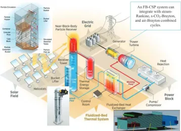
A traditional CSP plant runs either a Rankine (Steam) Power Cycle, a Brayton (commonly

air) Power Cycle or a combination of the two. Below in Figure 1 is an example of a modified

Rankine Power cycle (a) and a Brayton-Rankine combined cycle (b). In Figure 1a, the primary

working fluid is a gas that is heated in the concentrating tower. This gas then passes through a

heat exchanger, which heats the secondary working fluid, steam, which then passes through a

turbine to produce power. In Figure 1b, the primary working fluid is again a gas, but it first

passes through a turbine to produce power. After the gas is exhausted from the turbine, it still

holds a considerable amount of heat energy, enough in fact to power a Rankine cycle through

a heat exchanger.

In the literature, several papers discuss the use and optimization of power cycles

coupled with CSP plants. One such study optimized a CO2 Brayton cycle with molten salt

thermal energy storage utilizing a parametric approach [4]. Another, [5], discusses important

factors to be aware of in solar thermal Brayton cycles in order to prevent losses and focuses on

entropy minimization. Another paper studies and optimizes the effects of adding

nanometer-sized particles to the air stream to make the solar receive more efficient [6]. While these papers

discuss ways to make solar thermal Brayton cycles more efficient, they all use gases or

gas-particle suspensions as the primary working fluid. Some researchers have gone even further

and looked into using dense particle suspensions or dense granular flow particle fluids as the

primary working fluid in a solar thermal Brayton cycle [2], [7]. A layout of solar a thermal

Brayton cycle using particulate heat transfer fluids as the primary working fluid can be seen in

Figure 2.

Most technologies that utilize a particle heat transfer fluid rely on a secondary working

fluid to run the power cycle. There are generally two types of heat exchangers used to transfer

heat to the secondary working fluid; direct contact heat exchangers and indirect contact or shell

and tube heat exchangers. Many papers have been written which discuss direct contact heat

exchangers, such as fluidized bed heat exchangers [8]–[15] and packed bed heat exchangers

[16]–[20]. Although these are very efficient methods to transfer heat, they have their

drawbacks such as particulate loss and limited velocity and pressures of the gas. This work

focuses on indirect contact heat exchangers, particularly for use with thermal energy storage

devices. There are currently two main indirect contact heat exchanger designs used in

conjunction with a thermal energy storage medium. The main method utilizes an insulated

storage tank for the hot particles, which is connected to a shell and tube heat exchanger. The

particles flow with the help of gravity through the heat exchanger and transfer their heat as an

ordinary heat exchanger does [2],[21], [22]. The second method is to combine the storage tank

with the heat exchanger, i.e. run tubes through the packed particle bed, and, in a transient

manner, transfer heat to the secondary working fluid. This type of heat exchanger is referred

to as a thermocline heat exchanger, which contains a static fluid or solid with a temperature

gradient along its length. Several authors have written about thermocline heat exchangers used

with static particle beds. In [23] they discuss the effectiveness of thermocline heat exchangers.

In [20], [24], [25] a modified lumped capacitance model is developed to predict the transient

behavior of the static particle bed and the heat exchanger. The present work investigates a

similar style heat exchanger and develops a similar, albeit simpler, lumped capacitance model

3

Experimental Examinations

3.1

Single Tube Experiment

In order to better understand the indirect heat transfer between a static particle bed and

air flowing through a single thin walled tube, a set of experiments were designed to obtain a

baseline set of data to “tune” a CFD simulation. Additionally, this baseline data was used to

get an idea of how the particle bed behaved in a transient manner and to help guide the design

of a multi-tube heat exchanger.

3.1.1

Design Considerations

A static particle bed heat exchanger was designed using parameters scaled down from

a full size power plant. The particle bed heat exchanger was designed based on a simple Air

Brayton Cycle designed to output 50MWe. The single pass system consists of a compressor,

combustor/heat exchanger and turbine using air as the working fluid.

Pair_1, Tair_1, mdot_air

Pnet_GT Pair_2, Tair_2

Pair_3, Tair_3

Pair_4, Tair_4

Compressor Turbine

Combustor

qdot_GT_comb

An exit temperature of 𝑇_{𝑎𝑖𝑟_3}= 700°𝐶 was chosen as the desired temperature for the operation

of the Brayton Cycle. With this output and an assumed cycle efficiency of 40% the

requirements of the heat exchanger were determined. The results indicate that the heat

exchanger needs to accommodate a mass flow rate of 245.7 kg/s and allow 125MW of heat

transfer. Table 1 shows all the pertinent requirements of the full-scale heat exchanger.

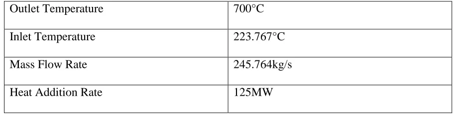
Table 1 Required Specifications of full-scale Heat Exchanger

Outlet Temperature 700°C

Inlet Temperature 223.767°C

Mass Flow Rate 245.764kg/s

Heat Addition Rate 125MW

Given these parameters, the optimum Reynolds number (𝑅𝑒_{𝐷,𝑜𝑝𝑡}) for the full-scale heat

exchanger was determined using an entropy minimization method for the air [26]–[28]. It was

decided that the heat exchanger would contain 1000 tubes, each 50 feet long.

𝑆′̇𝑔𝑒𝑛=

43.478 𝑞′2

𝜋 𝑘 𝑇2 _𝑃𝑟.04𝑅𝑒𝐷−.8+

. 0014375 𝜋3 _𝜇5

𝜌2 _{𝑇 𝑚̇}2 𝑅𝑒𝐷4.8 (1)

Here; k represents the thermal conductivity of air, Pr represents the Prandtl number of air, μ

represents the viscosity of air, ρ represents the density of air, T represents the average between

the desired outlet and inlet temperatures, 𝑞′ represents the heat addition rate per tube per length

of tube, and 𝑚̇ represents the mass flow rate per tube in the heat exchanger. Note that the air

properties are evaluated at T. Taking the derivate of 𝑆′̇_𝑔𝑒𝑛 with respect to the Reynolds number;

𝑅𝑒𝐷,𝑜𝑝𝑡 = 2.023 𝑃𝑟−.071 [

𝜌 𝑚̇ 𝑞′

𝜇2.5 _𝑘.5 _𝑇.5] .358

(2)

Based on this optimal Reynolds number, an optimal tube diameter was determined (Equation

3).

𝐷𝑜𝑝𝑡 =

4 𝑚̇_{𝑡𝑢𝑏𝑒}

𝑅𝑒𝐷,𝑜𝑝𝑡 𝜇 𝜋 (3)

The optimal Reynolds number was found to be approximately 2𝑒105 which is in the turbulent

regime. A turbulent flow is desirable in this case as it allows for higher heat transfer as

compared with a laminar flow. With the full-scale heat exchanger designed, an attempt was

made to scale it down to a lab-sized version. It was found that making a simplified version of

the heat exchanger consisting of a couple tubes while keeping the design Reynolds number the

same would be difficult and time consuming to build given the materials available. Therefore,

it was decided to build a single tube lab-scale heat exchanger with available materials while

keeping the Reynolds number in the turbulent regime.

3.1.2

Experimental Apparatus

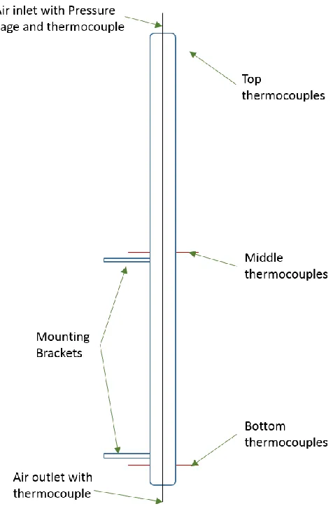
The single tube experiment apparatus consisted of two concentric stainless steel tubes

with a static particle bed in the annulus created between the two (Figure 4). The apparatus was

1.83m long which allowed well developed temperature gradients to be observed along the

length of the tube. Lengths of 1.83m tube were also easily accessible. The inside and outside

tube OD’s were 6.35mm and 50.8mm, respectively. The inside and outside tube ID’s were

4.57mm and 47.5mm, respectively. A series of spacer assemblies were distributed along the

0-100SLPM (standard liter per minute) Hastings HFC-203 flow meter was used in conjunction

with a Hastings power supply to control the airflow rate through the center tube. Due to the

large volume of particles required to fill the annulus between tubes, the system was setup to

“charge” the particle bed from a hot airflow. Heating roughly 9kg of particles uniformly and

in a time-efficient manner is a difficult task which would be required to study the discharge of

energy from the bed to the air. Although this is contrary to an actual TES heat exchanger, the

heat transfer between the air and particle bed can still be characterized and understood.

Therefore, the air entering the system was pre-heated using a 312W flexible heating tape. A

variable transformer was used to control the voltage supplied to the heating tape, allowing

different inlet temperatures to be obtained. In order to measure the temperature gradients in the

particles, three thermocouple clusters consisting of three type K thermocouples each were

used. The clusters were spaced evenly along the length of the tube assembly allowing enough

space on the ends to avoid end losses. The thermocouple clusters were axially spaced .826m

apart from one another and in the text, the author will refer to the topmost cluster as the top set

of thermocouples, the middle cluster as the middle set of thermocouples and the bottom cluster

Figure 4 Schematic of Single tube apparatus

The top set of thermocouples can be seen in Figure 5. In each thermocouple cluster, the

thermocouples were set radially 5.08mm, 10.16mm, and 15.24mm from the inner tube’s outer

wall. Three thermocouples were attached to the inner tube’s outer wall at these three axial

locations. Thermocouples were placed in the top and bottom of the 6.35mm tube to measure

the inlet and outlet air temperatures. A pressure gauge was placed at the inlet to measure the

pressure drop across the length of the tube. Finally, the entire apparatus was wrapped in

12.7mm of ceramic insulation and then 88.9mm of fiberglass insulation. A top view of the

the apparatus to show how the thermocouple assembly attaches to the outer tube. A mesh

screen is also visible over the top of the particle bed to prevent contamination. The heat source

for the air, as well as the air inlet thermocouple, can be seen in the figure as well.

Figure 5 Top View of Single Tube Apparatus

The particles used were chosen by the sponsor company, Research Triangle Institute

(RTI) International, and are composed of Zirconia-silica. They were selected because of their

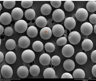
size, density, and ability to flow easily. The particles have a high spherocity, as can be seen in

Figure 6 Scanning Electron Microscope Image of 275-micron Zirconia-Silica particles

The particles have an average diameter of 300 microns but vary in size from 275

microns to 330 microns. A few of the bulk and individual properties of the particles are listed

in Table 2.

Table 2 Individual Particle and Bulk Particle properties

𝜌_{𝑝𝑎𝑟𝑡𝑖𝑐𝑙𝑒} 3934 𝑘𝑔/𝑚3

𝑘_{𝑝𝑎𝑟𝑡𝑖𝑐𝑙𝑒} 3 W/m*K (estimation for single particle)

𝜌𝑏𝑢𝑙𝑘 2386 𝑘𝑔/𝑚3

𝑘𝑏𝑢𝑙𝑘 .311 W/m*K (100°C)

𝑐𝑝,𝑏𝑢𝑙𝑘 598.13 J/kg*K (100°C)

3.1.3

Data Acquisition

As previously mentioned, 14 type K 20 gage exposed bead thermocouples were used

to record data. Nine of these thermocouples measure particle temperatures, three measure the

wall temperature of the 6.35mm tube and two measure the air inlet and exit temperature. An

Agilent 34970A Data Acquisition Logger utilizing an Agilent 34902A 16 channel card was

used to acquire temperature data. The program Benchlink Data Logger was used to record data

and export it to Microsoft Excel with a sampling period of one second.

Prior to starting a trial, the air controller had to be warmed up for 30 minutes. After this

period, the heating tape voltage source was set to the desired voltage and the data acquisition

program started. Trials usually lasted 8 hours to capture temperature profiles approaching

steady state. Figure 7 displays a typical data set of temperature measurements versus time for

the nine thermocouples surrounded by the particles and the inlet and exit air temperatures.

In the figure, Top 1 refers to the top cluster of thermocouples and is radially the closest

thermocouple to the 6.35mm tube in the top cluster, Top 2 is radially the second closest

thermocouple to the 6.35mm tube in the top cluster of thermocouples. The other thermocouple

names follow the same pattern. The breaks seen in the temperature profiles of Figure 7 are

periods where the data acquisition program was restarted. The noticeably lower temperatures

of the middle set of thermocouples is believed to be the result of heat loss from the main

mounting bracket which attaches to the apparatus directly beneath this middle thermocouple

measurement location. Ideally, in a perfectly insulated system, the steady-state particle bed

temperature would equal the incoming air temperature. This however, is not the case for the

current experiment as shown in Figure 7; there is ample evidence of heat loss out of the system.

3.2

Multi Tube Experiment

3.2.1

Design Considerations

In contrast to the single tube experiment, it was desired that the multi-tube experiment

involve discharging heat from the particles to the working fluid (air). In order to uniformly

heat a bed of particles in a timely manner, a relatively small bed of particles was required. An

oven [Vulcan 3-1750] was used to heat a particle bed and accompanying support structure

necessitating that the apparatus be sized to fit into the oven. In addition to deciding to operate

this unit to discharge heat to the air, an array of symmetric tubes in the heat exchanger was

designed where all temperature measurements are made around the center tube in the array. It

was determined that a 2D array of five tubes would be sufficient to ensure negligible heat

transfer between the center tube and surround tubes. As with the previous experiment, ensuring

important. Lastly, an array was desired so that thermally insulated boundaries could be

assumed on either side of the center tube, i.e. a section where symmetry boundary conditions

could be used to simplify the apparatus in simulations and analyses.

3.2.2

Design

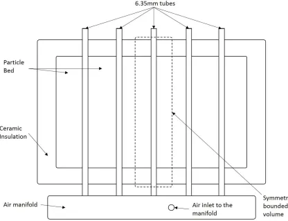
The multi-tube apparatus consisted of a .324 x .263 x .152 meter stainless steel

container wrapped with insulation and filled with particles. The apparatus used an array of five

6.35mm OD stainless steel tubes embedded in the particles, which were connected to a

manifold on one end and open to the environment on the other.

A second layer of 25.4mm ceramic insulation was applied to the outside of the

container to reduce heat loss. The 6.35mm tubes were inserted perpendicular to the long side

of the container at a spacing of 50.8mm (see Figure 8). A thermocouple was fixed just prior to

the inlet to the manifold to measure the inlet air temperature. It was assumed that this value

represents the inlet temperature of each individual tube. The outlet air temperature was

measured using a thermocouple fixed to the outlet of the center tube since the particle

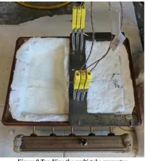
temperature measurements were made around the center tube. Figure 9 andFigure 10 show a

top view and side view, respectively, of the multi-tube experimental apparatus.

Figure 9 Top View the multi-tube apparatus

A “C” shaped piece of steel, which supported the thermocouples used to measure the particle

placement of the thermocouples from trial to trial. The steel plate was positioned using four

aluminum wedges that rested in slots cut into the plate and stainless steel container. The steel

plate had nine holes for thermocouples to allow for temperature measurement around the center

tube. The holes were grouped in clusters of three and were spaced radially in increments of

7.62mm. The clusters were spaced 72.1mm apart from one another in the axial air flow

direction. The first thermocouple hole in each cluster is located 7.62mm from the centerline of

the tube. All thermocouples are Type K exposed bead 20 gage thermocouples with a .81mm

sheath diameter and 152.4mm long sheath. In the text, the author will refer to the front and

back thermocouples. The front thermocouples are the ones closest to the air inlet and manifold

while the back thermocouples are the ones closest to the air outlet. This can be seen in Figure

10, where the right set of thermocouples are the front set and the left set are the back set.

3.2.3

Data Acquisition

This multi-tube experiment used the same data logging equipment as the single tube

experiment. Since this experiment required that the particles be preheated (i.e. charged), the

process for trials was quite different from that of the single tube experiment. First, the particles,

container, tubing, manifold, and inner insulation were heated to a desired temperature of

approximately 200°C. In order to reach that temperature in a reasonable time frame, the

apparatus was first heated at 350°C for 4 hours then removed to stir particles. The apparatus

was then heated again at 220°C for another 3 hours and removed. This left the particles at a

near uniform temperature of approximately 215°C. Once the particles and container were

heated, they were transferred to an insulating board where the thermocouple plate (steel plate)

was set in place. The thermocouples were then inserted into the particle bed through the

thermocouple plate and the inlet air was attached to the manifold. The outlet air thermocouple

was attached and 25.4mm of ceramic insulation was added to the sides and top of the apparatus.

Finally, the data logger was started and the air flow controller turned on to the desired flow

rate. Since this experiment takes 7-8 hours to preheat and setup, the data was collected

overnight over a 15-hour time span. The following morning, after the trial was completed, the

extra insulation was removed and the thermocouple locations in the particle bed were

uncovered and measured. To do this, half the particles were carefully removed to prevent the

thermocouples from shifting and the thermocouple beads were exposed to measure the actual

axial and radial locations of the beads. Since the thermocouple sheaths had such a small

diameter-to-length ratio, the thermocouples were fairly flexible and did not always enter the

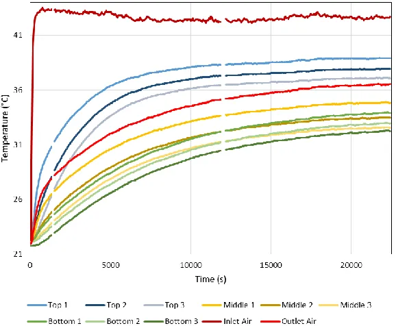
Figure 11 shows a typical temperature-time data set for the multi-tube experiment.

Figure 11 Temperature versus time graph for a typical trial run of the multi-tube discharging experiment

Note that the particle temperature profiles are all very similar and do not seem to vary

much based on radial or axial location. This observation, it suggests that the particles could be

represented by a lumped capacitance heat transfer model, which will be investigated in Section

5.

This observation for the multi-tube experiment is in contrast with the single tube

experiment’s behavior where well defined temperature gradients in both the axial and radial

directions exist. In an effort to determine the cause for this difference, the multi-tube apparatus

𝑚̇_𝑎𝑖𝑟 = . 000348𝑘𝑔/𝑠 𝑇_𝑠,𝑖 = 217°𝐶

was modified to allow charging trials be run. The modification was simple and involved taking

the heating tape from the single tube apparatus and attaching it to the air inlet tube of the

multi-tube apparatus. The process to run a trial for the modified multi-multi-tube apparatus (i.e. charging)

was the same as for the single tube experiment. It was found that when charging the particle

bed using the multi-tube apparatus, a temperature gradient was present similar to what occurs

when charging the single tube apparatus.

Figure 12 Temperature versus time graph for the modified multi-tube apparatus showing temperature gradients while charging particles

Figure 12 shows temperature gradients while charging the multi-tube particle bed which are

not present in the discharging multi-tube data. The significance of these results will be

discussed in more detail in Section 5.

𝑚̇𝑎𝑖𝑟 = . 000348𝑘𝑔/𝑠

𝑇𝑠,𝑖= 20°𝐶

4

ANSYS Simulation and Development

The computational fluid design program ANSYS Fluent was used for the development of

thermal simulations since it is very versatile, relatively user friendly and has a favorable

learning curve. The program is well adept at handling fluid flow and heat transfer problems,

and has an integrated meshing program. For the simulations developed here, the particle bed

was modelled as a solid having effective material and thermal properties of the particle bed,

rather than modelling individual particles surrounded by air. This greatly reduces the required

computing time for each simulation. Due to the low temperatures considered here (< 200°C),

radiation between the particles was assumed negligible.

4.1

Single Tube Simulation

4.1.1

Model Design and Meshing Parameters

When initially developing the model for the single tube experiment, a 3D geometry

consisting of the particles (treated as solid with effective properties), air, 6.35mm tube and

50.8mm tube was made. This initial geometry could not be used, however, due to meshing

complications such as hanging nodes and volumes not sharing a common boundary. Several

attempts were made to alter the geometry and obtain a good mesh but the problems persisted

for all but the simplest geometries. Eventually a 2D axisymmetric geometry was built which

included the air, 6.35mm tube, particles, 50.8mm tube, and outer insulation. This geometry

was capable of supporting a well-defined mesh with no hanging points or discontinuities. The

mesh and geometry worked well for the initial stages of developing the ANSYS Fluent model,

accounted for in ANSYS Fluent. Many simulations were run in an attempt to obtain results

similar to the experimental data. In these attempts, properties of the materials were altered,

boundary conditions were adjusted, and solution parameters were changed but nothing could

replicate the experimental data. Up to this point, the focus was on changing the ANSYS Fluent

settings. In reality, the geometry needed to be altered to account for heat loss from the main

support bracket (as discussed in Section 3.1.2). With this final alteration to the geometry and

minor adjustment of ANSYS Fluent parameters, the simulation data matched the experimental

data with a coefficient of determination of 0.99 or higher.

4.1.2

Fluent Parameters and Simulation

The simulation used a k-epsilon viscous model to represent the turbulent flow of air

inside the tube. Table 3 below lists the material properties used in the simulation.

Table 3 Properties for materials used in single tube simulation

Density (𝑘𝑔/𝑚3)

Specific Heat

(𝐽/𝑘𝑔 ∗ 𝐾) Thermal Conductivity (𝑊/𝑚 ∗ 𝐾) (𝑘𝑔/𝑚 ∗ 𝑠)Viscosity

Air 1.157 1006 0.0261 1.8705e-05

Insulation 72 843 0.03317 n/a

Steel 8030 503 16.17 n/a

Particles (Effective) 2386 545 0.292 n/a

The thermal conductivity and specific heat of a static particle bed were obtained from

the author’s colleague who measured the values directly at various temperatures using a Direct

Thermal Conductivity apparatus and a Differential Scanning Calorimeter, both from TA

instruments. The temperature dependence of both the thermal conductivity and specific heat

Figure 13 Dual graph of particle bed thermal conductivity and specific heat

A convective heat loss boundary condition with a coefficient of 5 𝑊/𝑚2𝐾 and a free

stream temperature of 22°C was applied to all external surfaces of the model. The air inlet had

a mass flow rate of .001𝑘𝑔/𝑠 , giving a Reynolds number of 1.49*10^4, with the air entering

at 42.5°C which was the average inlet temperature over the course of the trial from

experimental data. The air outlet was set to a gauge pressure of zero atmospheres and the

ambient temperature was 22°C. The solution was initialized defining the air inlet and setting

the entire system to an initial temperature of 22°C. The initial temperatures used for the

simulation were obtained from the experimental data being used to validate the simulation

results. While running, the simulation exported pressure and temperature data every two

y = -0.0007x2_{+ 0.9121x + 513.92}

R² = 0.9786

y = 0.0003x + 0.281 R² = 0.9932

0.000 0.100 0.200 0.300 0.400 0.500 0.600 0 100 200 300 400 500 600 700 800 900

0 100 200 300 400 500 600 700 800

Th erm al Con d u ctiv ity (W/m *K ) Sp ecif ic H eat (J /kg -K)

Temperature (°C)

Specific Heat (J/kg*K)

Thermal Conductivity (W/m*K) Poly. (Specific Heat (J/kg*K))

minutes which was then compared to the experimental data. Figure 14 below displays a

comparison between the simulation data and a corresponding set of experimental data.

Figure 14 Graph of experimental data versus ANSYS Fluent simulation for single tube charging apparatus

All simulation data sets were compared with experimental data and the coefficient of

determination was used as a measure for goodness of fit. Starting at the top tier thermocouples

and progressing to the bottom tier of thermocouples, the lowest coefficient of determination

was 0.990, 0.983, and 0.989 respectively. This shows that the heat transfer between the particle

bed and flowing air is well described and predicted by ANSYS Fluent for the single tube

4.2

Multi-Tube Simulation

The ANSYS simulation for the multi tube experiment used the final model settings from

the single tube simulation with the exception that the particle properties were adjusted for a

higher temperature. The development of the multi-tube simulation progressed in much the

same way the single-tube simulation did with a few exceptions, most notably, that the

simulation geometry was simplified to a cross section around the center tube assuming no heat

flux crosses the symmetry boundaries.

4.2.1

Model Design and Meshing parameters

The first attempts at creating the 3D geometry for the multi-tube experiment included

the entire apparatus but this approach resulted in either a poor mesh or the simulation time

being inconveniently long.

The final geometry modeled a section of the apparatus surrounding the center tube, as

shown in Figure 8 and Figure 15. It included the bulk particles, insulation, stainless steel tube,

and air.

4.2.2

Fluent Parameters and Simulation

Since the single tube simulation reproduced the behavior of the particle bed so well,

the multi-tube simulation used the parameters from the single tube simulation as a starting

point. Changes that were made to the simulation include changing the particle properties to

account for a higher film temperature, changing the inlet air mass flow rate, decreasing the

inlet air temperature and increasing the initial apparatus temperature. Table 4 lists the material

properties used for the multi-tube apparatus simulation.

Table 4 Properties for materials used in multi tube simulation

Density (𝑘𝑔/𝑚3)

Specific Heat (𝐽/𝑘𝑔 ∗ 𝐾) Thermal Conductivity (𝑊/𝑚 ∗ 𝐾) Viscosity (𝑘𝑔/𝑚 ∗ 𝑠)

Air .852 1017.5 0.0353 2.367e-05

Insulation 128.1 1.13 0.06 n/a

Particles 2386 632.7 0.325 n/a

Steel 8030 502.5 16.27 n/a

For the simulation, it was assumed that no heat flux crossed the faces perpendicular to

the x-axis in Figure 15 (for both the bulk particles and insulation), therefore symmetry

boundary conditions were used. Some notable parameters for the simulation are as follows; the

inlet air flow rate was .000347 kg/s, giving a Reynolds number of 4.08*10^3, the ambient air

temperature was 20°C, the convection coefficient on the exterior of the insulation was

The results from the simulation were found to agree relatively well with the

experimental data for the multi tube apparatus. Plots of the outlet air temperature and a

temperature within the particle bed (Front 1) from the experiment and simulation are shown in

Figure 16.

Figure 16 Comparison of experimental data with simulation data for multi-tube discharging case

Using the coefficient of determination as the measure of goodness of fit, all simulation

data sets were compared with experimental data sets. The air outlet and front particle

temperature data all had a coefficient of determination 0.97, while the back particle data sets

that the simulation has characterized the transient temperature behavior of the particles well.

The results for the single tube and multi-tube simulation also validate the use of bulk particle

thermal and material properties.

With the multi-tube simulation properly tuned, high temperature charging simulations

based off the modified multi-tube apparatus were run for use in the lumped analysis section.

These results are shown in Figure 17. The inlet air flow temperature was set to 217°C (which

is equivalent to the initial particle temperature in the discharging simulations) and the initial

particle temperature was set to 20°C. There was no experimental data with which to compare

the simulation data to for this case.

5

Simple Lumped Analysis Approximation

Due to the complexity and time it takes to develop the ANSYS simulations, a simple

lumped analysis solution was desired to predict the experimental outcomes with acceptable

accuracy. The solution was developed for both charging and discharging energy in a system

over time. A cross-section of the multi-tube experiment can be seen in Figure 18, showing a

single tube and the surrounding particles. The dashed lines represent the control volumes used

for developing the lumped analysis approximation.

Figure 18 Cross-section of multi-tube experiment showing single tube of air

The approximation starts with a simple energy balance on a control volume of air

(Figure 18).

𝑚̇_𝑎𝑖𝑟𝑐_𝑝,𝑎𝑇_𝑎,𝑥− 𝑚̇_𝑎𝑖𝑟𝑐_𝑝,𝑎(𝑇_𝑎,𝑥+𝑑𝑇𝑎,𝑥

Where 𝑚̇𝑎𝑖𝑟 is the air mass flow rate, 𝑐𝑝,𝑎 is the specific heat of air, ℎ𝑒𝑓𝑓 is the effective heat

transfer coefficient between the air and particle bed, 𝑃_𝑡 is the perimeter of the .00635m tube,

𝑇𝑎,𝑥 is the air temperature at different axial locations, and 𝑇𝑠(𝑡) is the lumped particle bed

temperature. For simplification purposes, let m be represented as the following.

𝑚 = 𝑃𝑡ℎ𝑒𝑓𝑓

𝑚̇𝑎𝑖𝑟𝑐𝑝,𝑎 (5)

Equation 4 can then rearranged as follows.

𝑑(𝑇𝑎)

𝑑𝑥 + 𝑚𝑇𝑎(𝑥) = m 𝑇𝑠(t) (6)

The solution to Equation 6 with the boundary condition given in Equation 7 results in Equation

8.

𝑇𝑎(𝑥)@𝑥=0= 𝑇𝑎,𝑖 (7)

𝑇_𝑎(𝑥) = 𝑇𝑠(𝑡) + (𝑇𝑎,𝑖− 𝑇𝑠(𝑡)) 𝑒−𝑚𝑥 (8)

The exit air temperature can be found by evaluating Equation 8 at the air outlet location (𝐿_𝑠)

as.

𝑇𝑎,𝑜 = 𝑇𝑠(𝑡) + (𝑇𝑎,𝑖 − 𝑇𝑠(𝑡)) 𝑒−𝑚𝐿𝑠 (9)

Because the air temperature is not constant along the length of the apparatus, a log mean

temperature difference is used to define the temperature difference experienced between 𝑇_𝑎,𝑖

∆𝑇_𝑙𝑚(t) =(𝑇𝑎,𝑜− 𝑇𝑠) − (𝑇𝑎,𝑖− 𝑇𝑠) ln (𝑇_𝑇𝑎,𝑜− 𝑇𝑠

𝑎,𝑖− 𝑇𝑠)

= 𝑇𝑎,𝑜− 𝑇𝑎,𝑖 ln (𝑇_𝑇𝑎,𝑜− 𝑇𝑠

𝑎,𝑖 − 𝑇𝑠)

₍₁₀₎

For further simplification, we will define the exponential term in Equation 9 as follows.

𝐶 = 𝑒−𝑚𝐿𝑠 = exp (−𝑃𝑡ℎ𝑒𝑓𝑓𝐿𝑠

𝑚̇𝑎𝑖𝑟𝑐𝑝,𝑎) (11)

Substituting Equation 9 into Equation 10 results in the following.

∆𝑇_𝑙𝑚(t) = 1 − 𝐶

ln(𝐶)(𝑇𝑠− 𝑇𝑎,𝑖) (12)

Figure 19 shows control volume occupied by the particles. The cross-sectional area, 𝐴_𝑐,𝑠, is

shown of the central tube by the hashed lines, and is simply the area occupied by particles

perpendicular to the x-axis.

Figure 19 View of apparatus showing lines of symmetry and cross-sectional area

An energy balance on the particles in the control volume containing the center tube

gives.

𝑑𝑈

Where U represents the internal energy of the system, 𝑞_{𝑐𝑜𝑛𝑣} represents the heat transferred to

the air flow, and 𝑞𝑙𝑜𝑠𝑠 represents the heat lost to the environment. The internal energy of the

system, can be rewritten as the product of the density (𝜌_𝑠), cross-sectional area (𝐴_𝑐), specific

heat (𝑐_𝑝,𝑠), length of particles (𝐿_𝑠), and temperature of the particles (𝑇_𝑠). The heat transfer from

the particles to the air can be written as the product of the effective heat transfer coefficient,

perimeter of the .00635m tube, length of the system, and the log-mean temperature difference.

The heat loss to the environment can be written as the product of the heat transfer coefficient

on the exterior of the insulation, the perimeter of the particle bed where heat is lost, the length

of the system, and the temperature difference between the particles and the environment.

Conservation of energy on the particle control volume gives.

𝑑(𝐴𝑐𝜌𝑠𝑐𝑝,𝑠𝑇𝑠𝐿𝑠)

𝑑𝑡 = ℎ𝑒𝑓𝑓𝑃𝑡𝐿𝑠∆𝑇𝑙𝑚− ℎ𝑖𝑛𝑓𝑃𝑜𝐿𝑠(𝑇𝑠 − 𝑇𝑖𝑛𝑓) (14)

The following variables are defined for simplification purposes.

𝐴 = ℎ𝑒𝑓𝑓𝑃𝑡

𝜌_𝑠𝑐_𝑝,𝑠𝐴_𝑐 (15)

𝐵 = ℎ𝑖𝑛𝑓𝑃𝑜

𝜌_𝑠𝑐_𝑝,𝑠𝐴_𝑐 (16)

Equation 14 can now be written as.

𝑑𝑇_𝑠 𝑑𝑡 = A

(1 − C)

ln(𝐶) (𝑇𝑠− 𝑇𝑎,𝑖) − 𝐵(𝑇𝑠− 𝑇𝑖𝑛𝑓) (17)

Equation 17 can be further reduced to the non-homogeneous ODE shown in Equation 19 by

𝐷 = A(1 − C)

ln(𝐶) (18)

𝑑𝑇_𝑠

𝑑𝑡 + (𝐵 − 𝐷)𝑇𝑠 = 𝐵𝑇𝑖𝑛𝑓 − 𝐷𝑇𝑎,𝑖 (19)

Solving the ODE using the initial condition shown in Equation 20 results in Equation 21.

𝑇_𝑠(𝑡)_@𝑡=0 = 𝑇_𝑠,𝑖 (20)

𝑇𝑠(𝑡) = (𝑇𝑠,𝑖 −

𝐵𝑇𝑖𝑛𝑓− 𝐷𝑇𝑎,𝑖

𝐵 − 𝐷 ) 𝑒−(𝐵−𝐷)𝑡+

𝐵𝑇𝑖𝑛𝑓− 𝐷𝑇𝑎,𝑖

𝐵 − 𝐷 (21)

The simple lumped analysis method was verified by comparing the predicted results to

experimental data from the multi-tube experiment as well to simulation data from the high

temperature multi-tube charging simulation. Each experimental data set (discharging case) was

fit to Equation 21 by adjusting the value of D, the coefficient of determination ranged from

0.955 to 0.997. The parameter D was averaged for all of the experimental data sets and was

used to determine an average ℎ𝑒𝑓𝑓. This average heat transfer coefficient was used to determine

an average temperature versus time curve, which was then compared to each experimental data

set. The average temperature curve has an average coefficient of determination of 0.972 when

compared to each experimental data, which is a reasonably good fit. The effective heat transfer

coefficient from this fit of D was found to be 50.7 𝑊/𝑚2𝐾. A plot of the average temperature

curve and the experimental data can be seen below in Figure 20. The high coefficients of

determination show that, even though some temperature gradients exist in the particles and air,

Figure 20 Plot of average temperature curve obtained from lumped analysis and experimental data presented in Figure 11 for the multi-tube discharging case

The lumped analysis equation was also fit to the high temperature simulation data

(charging case) for the multi-tube apparatus and was found to have similar results. The initial

fit had a goodness of fit in the range of .85 to .98. The average heat transfer coefficient was

found to be 84.1 𝑊/𝑚2𝐾, and the predicted average temperature curve fit the simulation data

with an average coefficient of determination of .87. A plot of the average temperature curve

Figure 21 Graph of the average temperature curve compared to simulation data presented in Figure 17 for a high temperature charging case

When examining the work of Xu et al. [24], it was noted that they validated their effective

heat transfer coefficient correlation based on matching the energy stored/transferred as a

function of time using the lumped analysis rather than on the temperatures of the solid. This

method appeared to be more accurate since temperature gradients will always exist in practical

low thermal conductivity beds when heat is being transferred. Based on this, it was decided to

use the energy transferred/stored to determine effective heat transfer coefficient and the

following equation from [24] was used.

𝑄∗

𝑠(𝑡∗) =

𝑄_𝑠(𝑡)

𝜌 𝑐 𝑉(𝑇 − 𝑇 ) = 1 −

𝑇𝑠(𝑡) − 𝑇𝑖𝑛𝑓

In Equation 22, 𝑄∗_𝑠(𝑡∗) represents the dimensionless energy stored in the particles as a

function of dimensionless time. 𝑄_𝑠(𝑡) was determined using ANSYS and is the internal energy

in the particles as a function of time.

𝑄_𝑠(𝑡) = 𝑈_𝑖 − 𝑈_𝑠(𝑡) (23)

Equation 21 was substituted into Equation 22 and then the right side of Equation 22 was fit to

the left side to find the effective heat transfer coefficient. For both the charging and discharging

cases, the coefficient of determination was at least .995 which shows good agreement. The plot

of the fits for both the charging and discharging case can be seen in Figure 22 and Figure 23,

respectively. This method predicted different effective heat transfer coefficients for the

charging and discharging case than matching the temperature-time histories. For the

discharging case, an effective heat transfer coefficient of 47.4 𝑊/𝑚2𝐾 was predicted which is

similar to the previous method’s value. For the charging case, however, an effective heat

transfer coefficient of 39.8 𝑊/𝑚2𝐾 was predicted which is almost half of the previous

method’s value of 84.1 𝑊/𝑚2_{𝐾. This difference in the effective heat transfer coefficients is}

believed to be due to the fact that there are more significant temperature gradients in the

Figure 22 Graph of the internal energy curve compared to simulation data in charging case

For the charging and discharging case, the Biot number was 34.2 and 40.8, respectively,

when defining the characteristic length as the volume of particles divided by the outer surface

area of the stainless steel tube. The coefficients of determination above prove that, even though

both Biot numbers are well out of the acceptable range for use of the lumped capacitance

method, the simple lumped analysis developed above is capable of adequately characterizing

the thermal transient behavior of a static particle bed as long as an appropriate effective heat

6

Effectiveness Calculation

Along with developing a simple correlation to predict the behavior of multi tube

experiment, an idea of how effective this type of heat exchanger is also desired. The basic

definition for effectiveness is the actual heat transfer divided by the maximum possible heat

transfer. 𝜀 = 𝐶ℎ(𝑇ℎ,𝑖𝑛− 𝑇ℎ,𝑜𝑢𝑡) 𝐶𝑚𝑖𝑛(𝑇ℎ,𝑖𝑛− 𝑇𝑐,𝑖𝑛) = 𝐶𝑐(𝑇𝑐,𝑜𝑢𝑡− 𝑇𝑐,𝑖𝑛) 𝐶𝑚𝑖𝑛(𝑇ℎ,𝑖𝑛− 𝑇𝑐,𝑖𝑛) (24)

Here, 𝐶_ℎ and 𝐶_𝑐 represent the heat capacities of the hot and cold sides, respectively, 𝐶_𝑚𝑖𝑛 refers

to the minimum heat capacity of the system, either 𝐶_ℎ or 𝐶_𝑐, and 𝑇_ℎ and 𝑇_𝑐 refer to the inlet

and exit temperatures of the hot and cold sides, respectively. The heat capacity for the particles

is defined as the product of the mass and specific heat, for the air side, the heat capacity is

defined as the product of the specific heat and mass flow rate divided by the total time. The

present analysis analyzes the effectiveness of a single tube both charging and discharging,

based on the control volume displayed in Figure 19. Since the current system utilizes only one

moving fluid, a slight variation of Equation 18 is required (Equation 19) [20], [30]–[32].

𝜀 =𝐶ℎ(𝑇𝑠,𝑖− ∫ 𝑇_𝑠(𝑡) 𝑡_𝑒𝑛𝑑 𝑑𝑡 𝑡𝑒𝑛𝑑 0 ) 𝐶𝑚𝑖𝑛(𝑇𝑠,𝑖 − 𝑇𝑓,𝑖𝑛) (25)

In the equation above, 𝑇_𝑠,𝑖 refers to the initial particle temperature, 𝑇_{𝑓,𝑖𝑛} refers to the air

inlet temperature, and 𝑡_𝑒𝑛𝑑 refers to the total time. Instead of using the final temperature of the

determined using the average temperature curve determined from the lumped analysis method

to represent 𝑇_𝑠(𝑡). Since some error exists between the average temperature curve and the

experimental data, the effectiveness will also have some associated uncertainty. For the system

examined in the present study, the particles demonstrate the lowest heat capacity, as it is more

than an order of magnitude smaller than that of the air. Given that the particles represent the

minimum heat capacity of the system, the effectiveness is easily evaluated from the perspective

of the particles. This will eliminate the heat capacities in the numerator and denominator in

Equation 24. Solving this equation for both the charging and discharging case results in an

effectiveness of approximately 78% and 77%, respectively, even though all they heat was

transferred out at the end of the trials. The integral in the numerator of Equation 25 essentially

takes the average particle bed temperature and uses it in the effectiveness expression. This

means that the effectiveness in Equation 25 is an average effectiveness over the duration of

7

Conclusion

In this study, the characteristics of ceramic particles used as a heat transfer medium were

studied using experimental and computational analyses. The work focused on using the

particles as a thermal energy storage medium and investigated potential heat

extraction/addition methods. In particular, a static bed heat exchanger was studied and the

transient heat transfer characteristics observed. Two experimental apparatuses were designed

and compared with ANSYS Fluent thermal simulations. It was observed that when charging

and discharging heat from a bed of particles, the bed exhibited a “lumped mass” like

temperature-time behavior. As such, a simple lumped analysis method was developed to

predict the behavior of the particle bed with relatively high accuracy. Our method used the

total energy transferred to the bed and accounted for heat loss to the environment. It proved

that using a lumped capacitance method with an effective heat transfer coefficient between the

particles and air is a valid method for characterizing the transient thermal behavior of a particle

bed heat exchanger.

Since this was a general study on the transient nature of the particles, there is room for

further study. Future work could include studying the behavior of the system at temperatures

at 1000°C to examine the effect of radiation. The applicability of a particulate heat exchanger

that possesses a time-dependent outlet air temperature in an industrial application could also

be investigated. If a transient outlet air temperature is not desirable for an industrial power

plant, is there a way to modify the system to be utilized for constant outlet air temperature.

8

REFERENCES

[1] A. C. Köberle, D. E. H. J. Gernaat, and D. P. van Vuuren, “Assessing current and future techno-economic potential of concentrated solar power and photovoltaic electricity generation,” Energy, vol. 89, pp. 739–756, 2015.

[2] Z. Ma, M. Mehos, G. Glatzmaier, and B. B. Sakadjian, “Development of a

concentrating solar power system using fluidized-bed technology for thermal energy conversion and solid particles for thermal energy storage,” Energy Procedia, vol. 69. pp. 1349–1359, 2015.

[3] “Solar Thermal Power Plants,” Renewable Energy World, pp. 109–113, 2003.

[4] J. D. Osorio, R. Hovsapian, and J. C. Ordonez, “Dynamic analysis of concentrated solar supercritical CO2-based power generation closed-loop cycle,” Appl. Therm. Eng., vol. 93, pp. 920–934, 2016.

[5] W. G. Le Roux, T. Bello-Ochende, and J. P. Meyer, “A review on the thermodynamic optimisation and modelling of the solar thermal Brayton cycle,” Renew. Sustain. Energy Rev., vol. 28, pp. 677–690, 2013.

[6] P. Fernández and F. J. Miller, “Performance analysis and preliminary design optimization of a Small Particle Heat Exchange Receiver for solar tower power plants,” Sol. Energy, vol. 112, pp. 458–468, 2015.

[7] H. Benoit, I. Pérez López, D. Gauthier, J.-L. Sans, and G. Flamant, “On-sun

demonstration of a 750°C heat transfer fluid for concentrating solar systems: Dense particle suspension in tube,” Sol. Energy, vol. 118, pp. 622–633, 2015.

[8] P. Basu and P. K. Nag, “An investigation into heat transfer in circulating fluidized beds,” Int. J. Heat Mass Transf., vol. 30, no. 11, pp. 2399–2409, 1987.

[9] R. S. Brodkey, D. S. Kim, and W. Sidner, “Fluid to particle heat transfer in a fluidized bed and to single particles,” Int. J. Heat Mass Transf., vol. 34, no. 9, pp. 2327–2337, 1991.

[10] “HEAT TRANSFER CHARACTERISTICS OF SHALLOW AND DEEP FLUIDIZED BEDS PACKED WITH HEAT EXCHANGERS.pdf.” .

[12] D. R. Mcgaw, “HEAT TRANSFER IN SHALLOW CROSSFLOW FLUIDIZED BED HEAT EXCHANGERS-II . EXPERIMENTAL describe the bulk contacting

characteristics of particles,” vol. 19, pp. 665–671, 1976.

[13] K. Pisters and A. Prakash, “Investigations of axial and radial variations of heat transfer coefficient in bubbling fluidized bed with fast response probe,” Powder Technol., vol. 207, no. 1–3, pp. 224–231, 2011.

[14] P. Kalita, P. Mahanta, and U. K. Saha, “Some studies on wall-to-bed heat transfer in a pressurized circulating fluidized bed unit,” Procedia Eng., vol. 56, pp. 163–172, 2013.

[15] H. L. Zhang, J. Baeyens, J. Degrève, A. Brems, and R. Dewil, “The convection heat transfer coefficient in a Circulating Fluidized Bed (CFB),” Adv. Powder Technol., vol. 25, no. 2, pp. 710–715, 2014.

[16] M. Cascetta, G. Cau, P. Puddu, and F. Serra, “A comparison between CFD simulation and experimental investigation of a packed-bed thermal energy storage system,” Appl. Therm. Eng., vol. 98, pp. 1263–1272, 2016.

[17] M. J. Baker, “CFD simulation of flow through packed beds using the finite volume technique,” Univ. Exet., p. 208, 2011.

[18] B. Xu, P. Li, and C. Lik Chan, “Energy Storage Start-up Strategies for Concentrated Solar Power Plants With a Dual-Media Thermal Storage System,” J. Sol. Energy Eng., vol. 137, no. 5, p. 51002, 2015.

[19] C. A. Kramer, O. Ghasemi-Fare, and P. Basu, “Laboratory Thermal Performance Tests on a Model Heat Exchanger Pile in Sand,” Geotech. Geol. Eng., vol. 33, no. 2, pp. 253–271, 2015.

[20] P. Li, J. Van Lew, C. Chan, W. Karaki, J. Stephens, and J. E. O’Brien, “Similarity and generalized analysis of efficiencies of thermal energy storage systems,” Renew. Energy, vol. 39, no. 1, pp. 388–402, 2012.

[21] A. El-Leathy, S. Jeter, H. Al-Ansary, S. Abdel-Khalik, J. Roop, M. Golob, S. Danish, A. Alrished, E. Djajadiwinata, and Z. Al-Suhaibani, “Thermal performance evaluation of two thermal energy storage tank design concepts for use with a solid particle

receiver-based solar power tower,” Energies, vol. 7, no. 12, pp. 8201–8216, 2014.

[23] P. Li, J. Van Lew, W. Karaki, C. Chan, J. Stephens, and Q. Wang, “Generalized charts of energy storage effectiveness for thermocline heat storage tank design and

calibration,” Sol. Energy, vol. 85, no. 9, pp. 2130–2143, 2011.

[24] B. Xu, P. W. Li, and C. L. Chan, “Extending the validity of lumped capacitance

method for large Biot number in thermal storage application,” Sol. Energy, vol. 86, no. 6, pp. 1709–1724, 2012.

[25] Y. Jian, F. Bai, Q. Falcoz, C. Xu, Y. Wang, and Z. Wang, “Thermal analysis and design of solid energy storage systems using a modi fi ed lumped capacitance method,” Appl. Therm. Eng., vol. 75, pp. 213–223, 2015.

[26] Y. Jaluria, Design and Optimization of Thermal Systems. McGraw-Hill, 1998.

[27] A. Bejan, Entropy Generation Minimization. The Method of Thermodynamic Optimization of Finite-Size Systems and Finite-Time Processes. CRC Press, 1995.

[28] A. Bejan, Entropy Generation Through Heat and Fluid Flow. John Wiley and Sons Inc., 1982.

[29] C. Ansys, “ANSYS CFX-solver theory guide,” ANSYS CFX Release, vol. 15317, no. April. pp. 724–746, 2009.

[30] F. Zaversky, M. Sánchez, and D. Astrain, “Object-oriented modeling for the transient response simulation of multi-pass shell-and-tube heat exchangers as applied in active indirect thermal energy storage systems for concentrated solar power,” Energy, vol. 65, pp. 647–664, 2014.

[31] T. Gao, B. G. Sammakia, S. Member, J. F. Geer, A. Ortega, and R. Schmidt,

“Dynamic Analysis of Cross Flow Heat Exchangers in Data Centers Using Transient Effectiveness Method,” vol. 4, no. 12, pp. 1925–1935, 2014.

[32] T. Gao, J. Geer, and B. Sammakia, “Development and verification of compact