Lateral Parameter Estimation of Aircraft with
Different Initial Conditions
Bijily Rose Varghese
1, Ms. Manju G
2PG Student [Control Systems], Dept. of EEE, MBCET, Trivandrum, India1 Assistant Professor, Dept. of EEE, MBCET,Trivandrum, India2
ABSTRACT: This paper aims to estimate the lateral aerodynamic parameters of the aircraft from the available measurements with different initial conditions. In this current work Filter Error Method (FEM) which accounts for both process and measurement noise, is used to estimate the lateral aerodynamic parameters from aircraft data. FEM algorithm is developed in MATLAB environment. With the developed algorithm studies are carried out at different instance of the aircraft and the estimated parameters are compared with wind tunnel predictions.
KEYWORDS: Aerodynamic parameter, Filter Error Method, Gauss Newton Method, Kalman Filter.
I.INTRODUCTION
Parameter estimation, is the subfield of system identification, which determines the best estimates of the parameters occurring in the model. Aircraft parameter estimation is the best example of system identification. An aircraft motion is described by equations of motion derived from the Newtonian mechanics, considering the vehicle as a rigid body. The aerodynamic forces and moments cannot be measured directly. However, aerodynamic modeling followed by parameter estimation helps to determine the aerodynamic parameters. Conventional methods of parameter estimation are (i)Equation Error Method[2] (ii) Output Error Methods (OEM)[3,4] and (iii) Filter Error Methods (FEM). Out of these methods Filter Error Method (FEM), is the most general stochastic approach for aircraft parameter estimation, which accounts for both process and measurement noise. In this current work Filter Error Method (FEM), is used to estimate the lateral aerodynamic parameters. FEM algorithm is developed in MATLAB environment. State estimation is carried out with Kalman Filter and the parameters are updated using Gauss Newton Method. With the developed algorithm studies are carried out at different instance of the aircraft and the estimated parameters are compared with wind tunnel predictions.
II. LATERAL DYNAMICS
Aircraft experiences aerodynamic forces and moments during their motion in atmosphere.
Fig. 1. Aerodynamic forces and moments
y Y
F
C qS
(1)Aerodynamic moments are given by (2)-(3)
L
C qSb
l (2)
N
C qSb
n (3)Where
q
is the dynamic pressure, S is the reference area, b is the lateral reference length,C C C
Y,
l,
n are the total side force coefficient, total rolling moment coefficient, and yawing moment coefficients.. The state equations are given from (4)-(8). 2 2 2 2 2 2 2(
)
(
)
(
)
u
w v v uu
ww
u
v
w
u
w
(4)
q
sin
r
cos
(5)
sin
( cos
sin )
cos
p
q
r
(6)2 2
(
)
(
)
(
)
(
)
l yz yy zz xy xz xxC qSb I q
r
rq I
I
I q pr
I r pq
p
I
(7)
2 2
(
)
(
)
(
)
(
)
n yx xx yy zx yz yyC qSb I p
q
pq I
I
I p qr
I q rp
r
I
(8)
Where
u v w
, ,
are the translational velocity,
p q r
, ,
are the body rates,
V
is
the vehicle velocity, ,
is the
side slip angle,
I
xx,
I
yy,
I
zzare the moment of inertia and
I
xy,
I
yz,
I
zxare the product of inertia,
,
are the
euler angles. The aerodynamic coefficients are modelled in linear form as:
C
Y
C
Y0
C
Y
C
Y e1
e1
C
Y e 2
e2
C
Y r1
r1
C
Y r 2
r2(9)
C
l
C
l0
C
l
C
l e1
e1
C
l e 2
e2
C
l r 1
r1
C
l r 2
r2(10)
C
n
C
n0
C
n
C
n e1
e1
C
n e 2
e2
C
n r1
r1
C
n r 2
r2(11)
where
C C C C
Y0, l0, n0, Y,
C
l,
C
nare the basic coefficients and
1,
2,
1,
2,
Y e Y e Y r Y rC
C
C
C
C
l e 1,
C
l e 2,
C
l r 1,
C
l r 2,
C
n e 1,
C
n e 2,
C
n r 1,
C
n r 2are the incremental coefficients
due to control surface deflections. Thus the unknown parameters to be estimated are given as:
0 1 2 1 2 0 1 2 1 2 0 1 2 1 2[
]
T Y Y Y e Y e Y r Y r l l l e l e l r l r n n n e n e n r n rC C C
C
C
C
C C C C
C C
C C C
C
C
C
(12)
Observation equations are given by (13)-(20)
m
(13)
m
(14)
m
(15)
p
m
p
(16)
r
m
r
(17)2 2
(
)
(
)
(
)
(
)
l yz yy zz xy xz
m
xx
C qSb I q
r
rq I
I
I q pr
I r pq
p
I
2 2
(
)
(
)
(
)
(
)
n yx xx yy zx yz
m
yy
C qSb I p q
pq I
I
I p qr I q rp
r
I
(19)
a
ymC qS
Ym
(20)Where, m is the mass of the vehicle,
m,
m,
m,
p r
m,
m are the sideslip angle, euler angles, and body rates,p r
m,
mare the measured angular accelerations and
a
ym are the measured acceleration.III. EFFECT OF INITIAL CONDITION
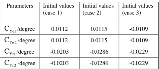
The effect of initial condition of the coefficient on the estimates is studied by considering different initial conditions. The different initial conditions are shown in table 1.
Table 1: Different initial conditions
Parameters Initial values (case 1)
Initial values (case 2)
Initial values (case 3)
Ye1
C
/degree 0.0112 0.0115 -0.0109Ye2
C
/degree 0.0112 0.0115 -0.0109Yr1
C
/degree -0.0203 -0.0286 -0.0229Yr 2
C
/degree -0.0203 -0.0286 -0.0229The presence of process noise makes Equation Error Method ,Output Error Method estimation techniques less efficient. Therefore, Filter Error Method [5] is used in this work which account for process and measurement noise. Since the system is stochastic in nature a steady state Kalman filter is used for obtaining the true state variables from the noisy measurements.
IV. RESULTS AND DISCUSSION
Fig. 2. Mach number, relative velocity, dynamic pressure and alpha during the estimation region.
Fig.3.Control surface deflections during the estimation region
0 5 10
2.6 2.7 2.8 2.9 3 Time(s) M a c h N um be r
0 5 10
4000 5000 6000 7000 Time(s) D y na m ic P re s s ure (P a )
0 5 10
800 820 840 860 880 Time(s) R e la ti v e V e loc it y (m /s )
0 5 10
15 16 17 18 19 Time(s) A lph a (de g)
0 5 10
-10 -8 -6 -4 -2 Time(s) Le ft E le v on D e fl e c ti on (de g)
0 5 10
-8 -6 -4 -2 0 Time(s) R igh t E le v on D e fl e c ti on (de g)
0 5 10
0 5 10 15 Time(s) Le ft R ud de r D e fl e c ti on (de g)
0 5 10
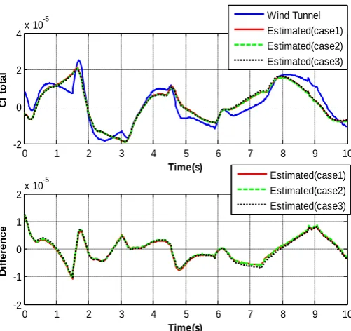
Fig. 4 The estimated total aerodynamic force coefficient
C
YFig. 5 The estimated total aerodynamic moment coefficient
C
0 1 2 3 4 5 6 7 8 9 10
-3 -2 -1
0x 10 -3
Time(s)
C
Y
t
ot
a
l
Wind Tunnel Estimated(case1) Estimated(case2) Estimated(case3)
0 1 2 3 4 5 6 7 8 9 10
-2 0 2 4
Time(s)
%
E
rr
or
Estimated(case1) Estimated(case2) Estimated(case3)
0 1 2 3 4 5 6 7 8 9 10
-2 0 2 4x 10
-5
Time(s)
C
l
tot
a
l
Wind Tunnel Estimated(case1) Estimated(case2) Estimated(case3)
0 1 2 3 4 5 6 7 8 9 10
-2 -1 0 1 2x 10
-5
Time(s)
D
if
fe
re
nc
e
Fig.6.The estimated total aerodynamic moment coefficient
C
n
V.CONCLUSION
Filter error algorithm is formulated and developed in MATLAB environment. With the developed algorithm lateral aerodynamic parameters are estimated with different noise levels .The estimated lateral aerodynamic coefficients are compared with wind tunnel prediction. Maximum of 3%, error, are observed in total aerodynamic force coefficients, 0.00001,0.000038 difference are observed in total aerodynamic moment coefficient.
REFERENCES
[1] R.E.Malne and L.W.Lfiff, “Identification of dynamic systems-applications to aircraft, part1-output error approach,” AGARDL flight test
techniques series, vol. 3, pp. 7-33, July 1986.
[2] Rakesh Kumar, “Lateral parameter estimation using regression”, International Journal of Engineering Inventions ISSN, vol. 1,pp: 76-81,
October2012.
[3] Luiz C.S.Góes, Elder M.Hemerly and Benedito C.O Maciel, “Parameter estimation and flight path reconstruction using output-error
method”,24th international congress of the aeronautical sciences,pp:1-10,2004.
[4] R V Jategaonkar and F Thieleckec, “Aircraft parameter estimation, A tool for development of aerodynamic databases,” Saadhanaa, Vol. 25,
Part 2, pp.119-135,April 2000.
[5] R.V Jategoankar, “Flight Vehicle System Identification : A time domain methodology ’’, volume 216, 2006.
0 1 2 3 4 5 6 7 8 9 10
-5 0 5x 10
-5
Time(s)
C
n
tot
a
l
Wind Tunnel Estimated(case1) Estimated(case2) Estimated(case3)
0 1 2 3 4 5 6 7 8 9 10
-4 -2 0 2 4x 10
-5
Time(s)
D
if
fe
re
nc
e