The Effects of Semantic Neighborhood Density on the Processing of Ambiguous Words

(1)

Electronic Thesis and Dissertation Repository

8-11-2014 12:00 AM

The Effects of Semantic Neighborhood Density on the Processing

of Ambiguous Words

Mark J. McPhedran

The University of Western Ontario Supervisor

Dr. Stephen J. Lupker

The University of Western Ontario

Graduate Program in Psychology

A thesis submitted in partial fulfillment of the requirements for the degree in Master of Science © Mark J. McPhedran 2014

Follow this and additional works at: https://ir.lib.uwo.ca/etd Part of the Cognition and Perception Commons

Recommended Citation Recommended Citation

McPhedran, Mark J., "The Effects of Semantic Neighborhood Density on the Processing of Ambiguous Words" (2014). Electronic Thesis and Dissertation Repository. 2416.

https://ir.lib.uwo.ca/etd/2416

This Dissertation/Thesis is brought to you for free and open access by Scholarship@Western. It has been accepted for inclusion in Electronic Thesis and Dissertation Repository by an authorized administrator of

(2)

THE EFFECTS OF SEMANTIC NEIGHBORHOOD DENSITY ON THE PROCESSING OF

AMBIGUOUS WORDS

by

Mark J. McPhedran

Graduate Program in Psychology

A thesis submitted in partial fulfillment of the requirements for the degree of Master of Science in Cognition & Perception

The School of Graduate and Postdoctoral Studies The University of Western Ontario

London, Ontario, Canada

(3)

Abstract

Semantic neighborhood density’s effects on the processing of ambiguous words were examined

in three lexical decision experiments. Semantic neighborhoods were defined in terms of semantic

set size and connectivity in Experiment 1, and in terms of semantic set size in Experiments 2 and

3. In Experiment 1, set size, connectivity, and ambiguity were crossed. An ambiguity

disadvantage was observed for large set, high connectivity words, and there was some suggestion

of an ambiguity advantage for small set, high connectivity words. Experiments 2 and 3 held

connectivity constant at a high level, and set size and ambiguity were crossed, with Experiment 3

using pseudohomophone nonwords. Neither experiment produced an ambiguity advantage.

Participants responded faster to unambiguous words relative to ambiguous words, particularly

for large set size words, essentially supporting Experiment 1’s results. These results are

discussed within a framework in which meaning-level competition can affect the recognition of

semantically ambiguous words.

(4)

ACKNOWLEDGEMENTS

I would like to express my sincere gratitude to my advisor Dr. Stephen Lupker for all of his

support during the writing of this thesis. His experience, guidance, and insight were instrumental

in the research and writing of this thesis, and I could not imagine having a better mentor and

advisor for this study.

I would also like to thank my fellow labmates: Dr. Jason Perry, Dr. Olessia Jouravlev, Jimmie

Zhang, and Arum Jeong for their guidance, encouragement, their insightful comments, and for

always challenging me with their difficult questions.

Last, but certainly not least, I would like to thank my parents, Cynthia and Stephen McPhedran,

for bringing me into this world and always supporting me throughout every step of my life. I

wouldn’t have been able to make it this far without the curiosity and love for knowledge that you

(5)

List of Tables

Table 1 - Mean Response Times (RTs) and Error Rates from Locker, Simpson, & Yates (2003), Experiment 1 ... 72 Table 2 - Mean Response Times (RTs) and Error Rates from Experiment 1 – Locker et al.’s (2003) stimuli – English Lexicon Project Database ... 73

Table 3 - Stimulus Characteristics from Experiment 1 ... 74

Table 4 - Mean Response Times (RTs) and Error Rates for Experiment 1 – Subject Analysis .... 75

Table 5 - Mean Response Times (RTs) and Error Rates for Experiment 1 – With Covariate ... 76

Table 6 - Mean Response Times (RTs) and Error Rates for Experiment 1 – English Lexicon Project ... 77

Table 7 - Mean Response Times (RTs) and Error Rates from Experiment 1 – Locker et al.’s (2003) stimuli ... 78

Table 8 - Mean Response Times (RTs) and Error Rates from Experiment 1 – New Stimuli ... 79

Table 9 - Mean Response Times (RTs) and Error Rates from Experiment 1 – New Stimuli – English Lexicon Project Database... 80

Table 10 - Number of Meanings (NOM) and Number of Senses (NOS) from Experiment 1-

Locker et al. (2003) stimuli ... 81

Table 11 - Number of Meanings (NOM) and Number of Senses from Experiment 1- New Stimuli

... 82

Table 12 - Stimulus Characteristics from Experiment 2 ... 83

Table 13 - Mean Response Times (RTs) and Error Rates from Experiment 2 – Subject Analysis 84

Table 14 - Mean Response Times (RTs) and Error Rates from Experiment 2 – Item Analysis .... 85

Table 15 - Mean Response Times (RTs) and Error Rates from Experiment 2 – English Lexicon Project Database ... 86

Table 16 - Stimulus Characteristics from Experiment 3 ... 87

Table 17 - Mean Response Times (RTs) and Error Rates from Experiment 3- Subject Analysis . 88

Table 18 - Mean Response Times (RTs) and Error Rates from Experiment 3- With Covariate ... 89

(8)

Table 20 - Experiment 1 Results – Early AoA words (AoA < 5.84) ... 91

Table 21 - Experiment 1 Results – Late AoA words (AoA > 5.84) ... 92

Table 22 - Experiment 2 Results- Early AoA Words (AoA < 5.62) ... 93

Table 23 - Experiment 2 Results - Late AoA Words (AoA > 5.62) ... 94

Table 24 - Experiment 3 Results- Early AoA Words (AoA < 5.44) ... 95

(9)

Introduction

There has been growing interest in the last few decades in how orthographic,

phonological, and semantic information are stored and activated during word reading. One

particular focus of this research has been examining how “neighborhood effects” influence the

process of visual word recognition. For example, extensive work has been done on the effects of

orthographic neighborhood size – defined as the set of words of the same length that differ from

that word by only one letter, (e.g., car and cot are neighbors of cat) – on visual word recognition

processes (e.g., Andrews, 1989, 1992; Coltheart, Davelaar, Jonasson, & Besner, 1977; Grainger,

1990; Grainger & Jacobs, 1996; Sears, Hino, & Lupker, 1995; Siakaluk, Sears, & Lupker, 2002).

Likewise, phonological neighborhoods – words that differ by a single phoneme from a specific

word – have also been extensively researched in an attempt to determine their role in word

recognition (e.g., Vitevitch, 2007; Yates, 2005, 2009; Ziegler, Muneaux, & Grainger, 2003).

In contrast, relatively little research has been done on semantic neighborhood effects. As

Buchanan, Westbury, and Burgess (2001) note, this dearth of research has stemmed in part from

several challenges in defining what constitutes a semantic neighbor. Whereas researchers have

reached some general consensus on reasonable definitions for what constitutes an orthographic

or phonological neighbor, there is no obvious way to define a semantic neighbor, because words

have many ways of being semantically related to each other. For example, an object-based view

of semantics defines semantic similarity in terms of the similarity of the objects themselves, be it

in terms of the amount of featural overlap shared by concepts (e.g., cat and dog are close

semantic neighbors because they share many semantic features, such as having four legs, fur, and

a tail), and/or in terms of being members of the same category of objects (e.g., McRae, Cree,

(10)

concepts as being semantically related on the basis of the statistical co-occurrence of the two

concepts regardless of the properties shared by the two objects. According to such a view, cat

and dog are near neighbors because they appear in similar contexts when large samples of

language are analyzed (e.g., global co-occurrence; Burgess & Lund, 2000; Landauer & Dumais,

1997; Lund & Burgess, 1996), or because the words are commonly used adjacent to each other in

everyday language (e.g., local co-occurrence; Nelson, McEvoy, & Schreiber, 1998), and

concepts can be semantically similar regardless of any similarity the objects themselves share.

Certainly, it may be the case that the space of semantic neighborhoods incorporates

properties of both object- and language-based semantics. As a result, semantic space would be

both very large and highly variable in structure. At worst, this would mean that the semantic

space can only be defined for any individual. More likely, however, while possessing a very

large and variable structure, such a semantic space may share characteristics across individuals.

For the purpose of the present thesis, it is assumed that while individual differences in semantics

do exist, the structure of this space is guided by general principles that influence how the space is

organized.

A central issue that the present research focuses on is the impact of a word’s semantic

neighborhood on the effects of semantic ambiguity. Semantically ambiguous words are those

having more than one meaning. In languages such as English, ambiguity is a highly prominent

feature of a person’s everyday linguistic environment in that a large majority of words in the

English language mean different things in different contexts. As such, ambiguity has been the

subject of much research and debate within the psycholinguistic literature over the last several

decades. Intuitively speaking, since ambiguity is such a ubiquitous feature of English, it would

(11)

space and, hence, on the process of visual word recognition. This idea is one that will be

developed in greater detail below. First, however, I will begin by discussing research that has

been done on both the effects of semantic neighborhood size and semantic ambiguity, as well as

some of the theoretical explanations of both of these effects. Finally, the main focus of this thesis,

the relationship between semantic ambiguity effects and semantic neighborhoods, will be

discussed.

Previous Research on Semantic Neighborhood Effects

Early research on semantic neighborhood effects has shown that the size and density of

semantic neighborhoods predict response times (RTs) in word recognition tasks. In the earliest

study of semantic neighborhood effects in visual word recognition, Buchanan et al. (2001)

quantified semantic space on the basis of Lund and Burgess’s (1996) hyperspace analogue to

language (HAL) model, a co-occurrence model of semantic memory. The HAL model constructs

a high-dimensional semantic space from a co-occurrence matrix, created by analyzing a massive

corpus of text. The model then encodes the contexts of word usage, as reflected in weighted

co-occurrences. The semantic neighborhood of a word corresponds to a group of words that are

close to it. A word’s neighborhood size is quantified either as how many words are within a

certain distance of the target word, or as the distance from the target word to a criterion number

of words, such as the 20th furthest word. The distance of neighbors around any particular word

varies, and this variance reflects the variance in the word’s “semantic density”. Using this metric,

Buchanan et al. found that words with denser neighborhoods produced faster response times in

both lexical decision and word naming tasks. A subsequent study by Siakaluk, Buchanan, and

(12)

Buchanan et al. (2001) offered a feedback activation account for these types of effects

based on the proposals of Balota, Ferraro, and Connor (1991). This account assumes that there

are distinct sets of reciprocally connected units dedicated to processing phonological,

orthographic, and semantic information. Activation of one of these sets of units subsequently

influences processing in the other sets of units through feedback, and the nature of this activation

determines the ease or difficulty of processing. A final assumption is that decisions in different

tasks will be based on the processing of different sets of units. The orthographic units would be

the locus of lexical decision making, the semantic units would be the locus of semantic

categorizations, and the phonological units would be the locus in naming tasks. In lexical

decision tasks, Buchanan et al. suggested that words with denser semantic neighborhoods are

processed faster as a result of enhanced feedback activation from the semantic units to the

orthographic units, causing the orthographic units to increase their activation more quickly.

Opposite Effects of Near and Distant Neighbors

Whereas earlier research on semantic neighborhood effects point to facilitative effects of

semantic neighbors, more recent research offers a finer grained analysis of the effects of

semantic neighbors on visual word recognition. Mirman and Magnuson (2008) suggested that

neighbors can simultaneously have both facilitative and inhibitory effects, rather than having

only one type of effect. They examined the independent effects of near and distant neighbors on

semantic access using a concreteness judgment task. Near neighbors are words having high

similarity, whereas distant neighbors have more moderate similarity. Their data showed opposite

effects for near and distant neighbors: words with many near neighbors were recognized more

slowly than words with few near neighbors, and words with many distant neighbors were

(13)

similar findings in word production tasks, finding higher semantic error rates for words with

many near semantic neighbors, and fewer semantic errors for words with many distant semantic

neighbors with aphasic patients, as well as with controls in a speeded picture-naming task.

Mirman and colleagues (Mirman, 2011; Mirman & Magnuson, 2008) argued that their

opposite effects are explainable within an attractor dynamics framework. In attractor models of

semantics (e.g., Cree, McRae, & McNorgan, 1999), attractors refer to stable states that

correspond to a concept’s combination of features. In such models, processing gravitates towards

the closest stable state or states, and is pulled more rapidly into a stable state as processing gets

closer to an attractor. Since near semantic neighbors are close to the target attractor, their

representations exert a pull just as processing is about to settle on the correct representation,

slowing the approach towards the target attractor. Because distant neighbors are farther from the

target, it is assumed that they would not induce such a high degree of competition. Further,

because the distant neighbors outnumber near neighbors, Mirman and Magnuson suggested that

the combination of small pulling effects from distant neighbors, pulling towards the vicinity of

the target, facilitates movement towards the attractor, overwhelming any impact of near

neighbors.

To test this account, Mirman and Magnuson (2008) analyzed simulations of another

attractor dynamics model of semantic processing (O’Connor, Cree, & McRae, 2009). Consistent

with the behavioral data that Mirman and Magnuson presented, they found that the attractor

model demonstrated detrimental effects of near neighbors and facilitative effects of distant

neighbors.

While the opposite effects of near and distant semantic neighbors have not been

(14)

(Mirman, 2011; Mirman & Magnuson, 2008) provide important insights into the dynamics of

semantic neighborhood effects. Recent research by Chen and Mirman (2012) has used a simple

interactive activation and competition (IAC) framework to simulate facilitative-inhibitive effect

reversals, and attempted to develop a unified account of the computational principles that govern

whether neighbor effects will be facilitative or inhibitory. Their model exhibited opposite effects

of near and distant semantic neighbors on word recognition and word production. In the word

recognition task, the model was slower to settle when the target word had many near semantic

neighbors, and was faster when the target had many distant semantic neighbors. Likewise, in

their word production simulations, word activation was slower for words with many near

semantic neighbors, and faster for words with many distant semantic neighbors. Overall, there

was a general trend that determined whether neighbor effects were facilitative or inhibitory:

strongly activated neighbors have a net inhibitory effect, while weakly active neighbors have a

net facilitative effect.

The present experiments attempted to extend the investigation of how neighbors exert

their effects in different circumstances. Of particular interest is examining whether semantic

neighborhood dynamics exert an influence on the strength and direction of another semantic

effect, specifically, semantic ambiguity, a semantic effect that has garnered much research

interest over the past several decades.

Previous Research on Semantic Ambiguity

The first studies to examine the effects of semantic ambiguity on visual word recognition

were conducted by Rubenstein and colleagues (Rubenstein, Garfield, & Millikan, 1970;

Rubenstein, Lewis, & Rubenstein, 1971), who found that homographs (i.e., words with the same

(15)

lexical decision tasks, which was later replicated by Jastrzembski (1981). However, these

findings were criticized by Gernsbacher (1984), who argued that ambiguous words are typically

more familiar than unambiguous words, and the faster response times for ambiguous words is

merely caused by a confound with familiarity. Once word familiarity was taken into account, she

found no effect of ambiguity. Since then, however, a number of studies have found a significant

facilitative effect for ambiguous words (i.e., an ambiguity advantage) in lexical decision tasks

(e.g., Hino & Lupker, 1996; Kellas, Ferraro, & Simpson, 1988; Millis & Button, 1989; Pexman

& Lupker, 1999), and naming tasks (e.g., Lichacz, Herdman, LeFevre, & Baird, 1999; Hino,

Lupker, & Pexman, 2002; Hino, Lupker, Sears, & Ogawa, 1998; Rodd, 2004; although see

Borowsky & Masson, 1996, for contradictory results) after controlling for familiarity. In contrast,

some studies have reported an ambiguity disadvantage when certain types of semantic

categorization tasks are used (Hino et al., 2002), or in an auditory lexical decision task when the

ambiguous stimuli used had multiple unrelated meanings (Rodd, Gaskell, & Marslen-Wilson,

2002, 2004). Given such inconsistencies, it is clear that understanding how readers deal with

semantic ambiguity presents a special challenge in psycholinguistic research.

Hino and Lupker (1996) and Pexman and Lupker (1999) argued that the ambiguity

advantage seen in lexical decision tasks can be explained in terms of the semantic feedback

account that was discussed above (Balota et al., 1991). As with having large, dense semantic

neighborhoods, words with multiple meanings are assumed to possess a more enriched semantic

representation, and should thus produce enriched semantic feedback from the semantic level to

the orthographic level.

To test this idea, Pexman and Lupker (1999) conducted two lexical decision experiments

(16)

pseudowords vs. pseudohomophones). Pexman and Lupker argued that the homophony effect –

the finding that homophones (e.g., maid) are responded to slower than nonhomophones – is also

quite consistent with a feedback model’s predictions. Homophones have one phonological code

that would feed back activation to multiple orthographic codes (e.g., for made and maid), which

would create competition at the orthographic level, ultimately slowing processing. Further,

Pexman and Lupker predicted: a) that if a feedback mechanism can account for the effects of

ambiguity and homophony, then the effects should co-occur in a lexical decision task; and b)

they should both increase in size when pseudohomophones are used because using

pseudohomophones should increase the activation necessary for a lexical representation to

trigger a “word” response. The results of their experiments supported their predictions. These

results provide support for a feedback account of the ambiguity advantage as well as the

homophone disadvantage in lexical decision.

Parallel Distributed Processing (PDP) Approaches to Explaining Semantic Ambiguity

Other research has directly examined the ability of parallel distributed processing (PDP)

models to account for the ambiguity advantage in lexical decision tasks, under the assumption

that performance is based on the nature of semantic coding. In such models (e.g., Borowsky &

Masson, 1996; Kawamoto, Farrar, & Kello, 1994; Plaut & McClelland, 1993; Plaut, McClelland,

Seidenberg, & Patterson, 1996; Rodd et al., 2004; Seidenberg & McClelland, 1989; Van Orden,

Pennington, & Stone, 1990), it is assumed that orthographic, phonological, and semantic

information for a word are not captured by individual processing units, but by unique patterns of

activation across sets of processing units representing these different domains. These units are

assumed to share interconnections with each other, and as the learning process occurs, the sets of

(17)

phonology or meaning) that is correctly associated with the orthographic input. Finally, it is

assumed that the consistency of this input-output relationship determines the strength of

association, which determines how quickly the model can settle on a correct output, and, as such,

predict that the speed and efficiency of phonological and semantic coding depends on the nature

of the orthographic-phonological and orthographic-semantic relationships of the words.

PDP models attempting to explain the ambiguity advantage in terms of semantic

activation would seem to face some difficulty because ambiguous words must, by definition,

have multiple different patterns of activation amongst the semantic units. Therefore, one would

expect competition, which would prolong settling time. In fact, as Joordens and Besner (1994)

have pointed out, such models do typically predict a processing time disadvantage for ambiguous

words due to the settling process being more difficult for words with these one-to-many

orthographic-semantic relationships; a prediction that is, of course, is inconsistent with the body

of empirical research showing an ambiguity advantage.

Nevertheless, models have emerged that attempt to explain the ambiguity advantage

specifically using PDP principles in constructing semantic representations. For example,

Joordens and Besner (1994) found that learning ambiguous words led their model to fail to settle

into one of the meaning patterns, and instead settled into a blend state in which there was a

mixture of the two learned meaning patterns. However, by using the number of processing cycles

to settle on any pattern in their simulations as a metric of lexical decision response latencies, they

found an ambiguity advantage.

An alternative way to explain the ambiguity advantage within a distributed

representational framework has been to assume that actual performance in lexical decision tasks

(18)

Kawamoto et al. (1994) assumed that simulating a lexical decision task required the orthographic

units, rather than the meaning units, to settle on a stable pattern of activation. They simulated the

ambiguity advantage in lexical decision tasks using a recurrent PDP network that used a least

mean square learning algorithm. When presented with ambiguous words, instead of modifying

the weights between orthographic and meaning units, their model strengthened the connection

weights between orthographic units. Using the number of cycles required for settling in the

orthographic module as a metric for performance in lexical decision, Kawamoto et al. found that

orthographic units settled more quickly for ambiguous words because the connection weights

between orthographic units had been strengthened in compensation for the weaker associations

between orthographic and semantic units.

The Issue of the Relatedness of the Multiple Meanings

An additional issue that researchers have investigated concerning the ambiguity effect

has been the relatedness of the meanings of ambiguous words (Azuma & Van Orden, 1997;

Rodd et al., 2002, 2004). Azuma and Van Orden factorially manipulated the relatedness of

meanings (ROM) and the number of meanings (NOM) possessed by their ambiguous words in

lexical decision tasks. Their results indicated that, while NOM was not a reliable predictor of

latencies, a significant main effect of ROM was found when pseudohomophone nonwords were

used. Given these findings, Azuma and Van Orden argued that the relatedness among meanings

can influence lexical decision times.

This approach was extended by Rodd et al. (2002). The large majority of studies

examining semantic ambiguity have not distinguished between what are regarded as the two

types of ambiguous words, referred to as homonyms and polysemes. Rodd et al. suggested that

(19)

bark, or bank, whereas polysemes refer to words with a variety of different senses, such as twist.

The crux of their argument was that, while having multiple word senses would produce an

ambiguity advantage, having multiple unrelated meanings would induce meaning-level

competition that would delay word recognition, consistent with what a PDP model might predict.

To test this prediction, Rodd et al. manipulated the type of ambiguity by referring to the

dictionary entries of words to classify words as having either multiple meanings or multiple

senses. Consistent with this idea, Rodd et al. reported an ambiguity advantage for words with

multiple senses when pseudohomophones were used in a visual lexical decision task and an

ambiguity disadvantage for words with unrelated meanings in an auditory lexical decision task.

Subsequently, Rodd et al. (2004) implemented a connectionist model to simulate these

findings. The simulations that they reported showed that words with multiple, unrelated

meanings such as bark demonstrated an ambiguity disadvantage, while words with multiple

senses demonstrated an ambiguity advantage. They explained these effects in terms of the

principles of attractor dynamics. They suggested that the ambiguity disadvantage occurs in

words with multiple meanings because these separate meanings correspond to separate attractor

basins in different regions of semantic space, resulting in a blend state during early activation

that the system must move away from before it can properly settle into one of the different

meanings. In contrast, the semantic representations of words with multiple senses correspond to

highly overlapping regions of semantic space. As a result, there is a larger area of semantic space

that corresponds to the meaning of these words, and this broader attractor basin aids the system

in settling, at least initially.

Support for Rodd et al.’s (2002, 2004) argument has been mixed. Some studies have

(20)

Fiorentino, & Poeppel, 2005; Klepousniotou & Baum, 2007) using Rodd et al.’s (2002) stimuli,

while others have found equivalent ambiguity advantages for both polysemes and homonyms in

lexical decision tasks (e.g., Hino, Pexman, & Lupker, 2006; Hino, Kusunose, & Lupker, 2010;

Klein & Murphy, 2001, 2002). For example, Hino et al. (2006) examined the relatedness of

meaning effect using lexical decision and semantic categorization tasks with Katakana-written

ambiguous words. Hino et al. obtained relatedness of meaning ratings of ambiguous words to

find words that could be classified as homonyms (i.e., essentially unrelated meanings) or

polysemous (generally related meanings). The result of their lexical decision experiment was that

there was no difference between homonyms and polysemes in their lexical decision latencies,

finding an equivalent ambiguity advantage for the two types of ambiguous words. These results

were replicated by Hino et al. (2010), who found equivalent ambiguity advantages for polysemes

and homonyms using both Katakana and Kanji words and nonwords.

Semantic Neighborhoods and Ambiguity

Given the abundance of evidence contrary to the claims of any PDP models that try to

explain ambiguity effects in terms of settling at the semantic level, semantic ambiguity continues

to present a major challenge for any PDP account of semantics. At the same time, however, the

results from ambiguity experiments have not been entirely consistent with other models either.

One possible explanation is that there has been little consideration of how ambiguous words

interact within the constraints of their semantic space. Indeed, as noted before, some theorists

(e.g., Buchanan et al., 2001) have suggested that semantic neighborhood effects are highly

similar to ambiguity effects, in that both concepts involve multiple items being simultaneously

activated at the semantic level. Further, it is likely that semantic ambiguity is represented in

(21)

meanings, such as bark. Bark occurs in some contexts when referring to the outer layer of a tree,

and in other contexts when referring to the sound that a dog makes. Such words will likely have

semantic neighbors related to both of these senses. At present, there appears to be only one study

that has examined semantic neighborhood effects on the processing of ambiguous words, Locker,

Simpson, and Yates (2003).

Locker et al. (2003) argued that it should be possible to induce semantic-level

competition between the multiple meanings of an ambiguous word if the magnitude of activation

of the different meanings is increased. Words with more meanings, they surmised, would have

richer representations in semantic memory, and would be more strongly activated. Such strong

activation, they argued, may also cause the multiple meanings to interfere with each other. Such

competition would reduce the strength of semantic feedback, or cause the feedback to be

inconsistent. As such, Locker et al. predicted that an ambiguity advantage would more likely be

observed when the meaning-level activation for secondary meanings is weak.

Locker et al. (2003) tested this idea by using two semantic neighborhood metrics to

estimate of the strength of activation of the meanings of an ambiguous word. Specifically, they

used semantic set size and network connectivity, derived from Nelson et al.’s (1998) free

association norms, as their measure of semantic neighborhood density/meaning activation. The

semantic set size in Nelson et al.’s norms is derived from presenting participants a list of words

and recording a single response that is meaningfully related to each target. The number of

responses across participants comprises the word’s set. For example, according to these norms,

the word dog has a set containing the words cat, animal, puppy, friend, and house, and thus has a

set size of five. At the same time, there are two associative connections among dog’s neighbors

(22)

associative connections within the neighborhood divided by the total neighborhood size. Since

dog has a set size of five, and there are two associative connections within dog’s neighborhood,

dog would have a connectivity of .40.

In their most relevant experiment, Locker et al. (2003) manipulated ambiguity

(ambiguous or unambiguous), semantic set size (large or small), and neighborhood connectivity

(high or low). Since Locker et al. predicted that the ambiguity advantage would only arise when

meaning-level activation is relatively weak, they predicted that an ambiguity advantage would be

most likely to arise when the semantic set size was small and neighborhood connectivity was low.

These predictions were borne out, as an ambiguity advantage only arose for words with low

connectivity and small set sizes. Locker et al.’s results can be found in Table 1.

Locker et al.’s (2003) results suggest that semantic neighbors may have some influence

over the strength and direction of other semantic effects. However, although Locker et al.’s

results suggest that semantic neighbors influence the strength and direction of the ambiguity

effect, they also raise a number of questions about the nature of ambiguity effects. Thus, the

main purpose of the present investigation was to expand on previous work done by Locker et al.

and Mirman and colleagues (Chen & Mirman, 2012; Mirman, 2011; Mirman & Magnuson,

2008). The studies reported below were designed to investigate how the organization of semantic

neighborhoods influences the strength and direction of the ambiguity effect, and whether the

inconsistencies in the literature on the ambiguity advantage can be accounted for in light of

semantic neighborhood dynamics.

Experiment 1

Experiment 1 was an attempt to replicate the results of Locker et al.’s (2003) Experiment

(23)

each cell of the design. The essential purpose of Experiment 1 was to evaluate Locker et al.’s

claim that the ambiguity advantage was restricted to small set size, low connectivity words (i.e.,

it was an attempt to replicate their three-way interaction). Their argument, again, is that if

increasing the scope of activation by manipulating connectivity reflects an increase in

competition, an ambiguity advantage should be observed when the scope of activation is

particularly low, specifically when the neighborhood set size is small and connectivity is

relatively low. Conversely, in cases where the scope of activation is extremely high, as when the

neighborhood size is large and the semantic connectivity is high, the greater scope of semantic

activation could be detrimental to the processing efficiency of semantically ambiguous words. If

increasing the scope of activation of the multiple meanings of an ambiguous word results in

greater semantic-level competition, one possibility is that there would be an inhibitory effect for

those ambiguous words. Locker et al. did not find this result, instead finding a small (~11 ms)

ambiguity advantage, yet the English Lexicon Project (ELP; Balota, Yap, Cortese, et al., 2007)

produced a sizable (~26 ms) inhibitory effect for ambiguous words with large set sizes and high

connectivity for Locker et al.’s stimuli. The ELP database results for Locker et al.’s stimuli are

shown in Table 2. Given the results from the ELP database, one might even expect that

ambiguous words with large, highly interconnected semantic neighborhoods will produce an

inhibitory effect.

Beyond the results in that cell, however, there are also other reasons to wonder about the

stability of Locker et al.’s (2003) results. First, the results produced by the ELP database (Balota

et al., 2007) for Locker et al.’s Experiment 1 stimuli failed to replicate Locker et al.’s pattern

concerning the ambiguity advantage. Although there was evidence in the ELP database

(24)

advantage was for words with small set sizes and high connectivity. In addition, there is the

simple fact that the ambiguity advantage has been replicated many times over the past several

decades (e.g., Hino & Lupker, 1996; Kellas et al., 1988; Millis & Button, 1989; Pexman &

Lupker, 1999), and it seems unlikely that those researchers would have, just by chance, selected

only ambiguous words with small semantic set sizes and low connectivity. Therefore, it is far

from clear that Locker et al.’s findings will successfully replicate, and that it may be the case that

the advantage for ambiguous words may be more widespread than their results suggest.

Method

Participants. Participants were 52 undergraduate psychology students at the University

of Western Ontario, who participated in this study for course credit, or were compensated

monetarily. The data from 10 participants were excluded from the experiment on the basis of

excessive error rates (>15% for word stimuli, or >20% for nonword stimuli). Thus, the analyses

reported are based on the data from 42 participants. All participants had normal or

corrected-to-normal vision, and all were native English speakers.

Stimuli. For the word trials, a 160-word list formed by crossing semantic ambiguity

(ambiguous or unambiguous), set size (large or small) and connectivity (high or low) was used.

All of the words included in this study can be found in the University of South Florida Word

Association, Rhyme, and Word Fragment Norms (Nelson et al., 1998). Half of the word stimuli

used in this study were used in Locker et al.’s (2003) Experiment 1, and the other half were

selected from previous studies based on normative data (e.g., Twilley, Dixon, Taylor, & Clark,

1994). Consistent with Locker et al., words with a number of associates greater than 15 were

classified as large set (M = 19.26), whereas words with associates numbering 14 or fewer were

(25)

greater (M = 2.20), whereas low-connectivity words all had fewer than 1.5 connections (M =

0.85). All word types were equated in terms of length, CELEX frequency, and orthographic

neighborhood size using N-watch (Davis, 2005), and concreteness using the MRC

psycholinguistic database (Coltheart, 1981). Additionally, data on the age of acquisition (AoA)

of all the word stimuli using norms developed by Kuperman, Stadtagen-Gonzalez, and Brysbaert

(2012) were collected. AoA is known to be a strong predictor of performance on a variety of

linguistic tasks (e.g., Catling, Dent, & Williamson, 2008; Catling & Johnston, 2005, 2006;

Coltheart, Laxon, & Keating, 1988; Cortese & Schock, 2013; Johnston & Barry, 2005) and it had

not been equated by Locker et al. As a result, it was not possible to equate the words fully on

AoA in our set of stimuli as well, a problem that was addressed by doing an analysis of

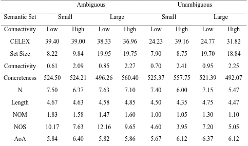
covariance (ANCOVA). The stimulus characteristics for each condition are shown in Table 3.

The stimuli are shown in Appendix A. In addition, 160 orthographically legal nonwords were

used, which were equated with the word stimuli in terms of length and orthographic

neighborhood size. An additional 5 words and 5 nonwords that did not appear in the

experimental trials were presented as practice trials for each participant.

Procedure. Stimuli were presented on a LG Flatron W2242TQ-BF LCD monitor.

Recording of response latencies and accuracy was controlled using DMDX software (Forster &

Forster, 2003). At the beginning of each trial, a fixation stimulus (#####) appeared in the middle

of the screen for 750 ms. The stimulus was then removed, and a word or nonword was presented

in uppercase letters. The target remained on the screen until the participant responded. Lexical

decisions were made by pressing the / key for words and the z key for nonwords. Presentation of

(26)

Results and Discussion

Mean lexical decision latencies and error rates for both participants and items were

submitted to a 2 (semantic ambiguity: ambiguous vs. unambiguous) x 2 (semantic set size: large

vs. small) x 2 (connectivity: high vs. low) repeated-measures analysis of variance (ANOVA)

based on subjects, and a between-word ANOVA based on items. Outliers were defined as

latencies shorter than 250 ms or longer than 1,500 ms and were removed from all analyses. Five

word stimuli and 5 nonword stimuli were also excluded from the analyses due to excessive error

rates (>15% for word stimuli, or >20% for nonword stimuli). For the item analysis, AoA was

treated as a covariate. Mean response latencies and error percentages for each word condition in

the subject analysis are reported in Table 4 (without AoA as a covariate), and Table 5 contains

the means from the item analysis with the covariate. As can be seen, the impact of treating AoA

as a covariate on the pattern of results was minimal. Additionally, we calculated mean RTs for

all of the word stimuli using the English Lexicon Project database (ELP; Balota et al., 2007).

Table 6 provides the mean response latencies and error percentages based on those data.

There were no significant main effects in the latency analyses. The interaction between

ambiguity and semantic set size approached significance in the subject analysis, but was not

significant in the item analysis, F1(1, 41) = 3.62, p < .10, F(1, 145) = 1.55, p < .30. The

interaction between set size and connectivity was highly significant in the subject analysis, but

not in the item analysis, F1(1, 41) = 10.79, p < .005, F2(1, 145) = 1.05, p < .50. Finally, a

significant three-way interaction was found between ambiguity, semantic set size, and

connectivity in both analyses, F1(1, 41) = 15.83, p < .001, F2(1, 145) = 5.28, p < .05.

Simple main effects analyses were undertaken to determine which cells show a

(27)

high connectivity (M = 611) were processed significantly faster than their ambiguous

counterparts (M = 639) in both the subjects and item analyses, F1(1, 41) = 18.65, p < .001, F2(1,

145) = 6.46, p < .05. No other differences reached significance (all Fs < 2.7).

In the error analyses, the main effect of connectivity approached significance in the

subject analysis, F1(1, 41) = 3.18, p < .10, but not in the item analysis F2(1, 145) = 2.62, p = .11,

as high connectivity words had slightly lower error rates overall. A two-way interaction between

ambiguity and semantic set size was found in both analyses, F1(1, 41) = 8.10, p < .01, F2(1, 145)

= 4.22, p < .05. A two-way interaction was also found between ambiguity and connectivity, F1(1,

41) = 5.69, p < .05, F2(1, 145) = 9.54, p < .005. Finally, the three-way interaction between

ambiguity, semantic set size, and connectivity approached significance in the subject analysis,

but did not in the item analysis, F1(1, 41) = 3.72, p < .10, F2(1, 145) = 1.65, p = .20.

Simple main effects analyses showed that ambiguous words with small set sizes and high

connectivity (M = 1.63%) produced significantly fewer errors than unambiguous words with

small set sizes and high connectivity (M = 5.24%) in both analyses, F1(1, 41) = 15.55, p < .001,

F(1, 145) = 14.72, p < .001. No other differences reached significance (all Fs < 2.5).

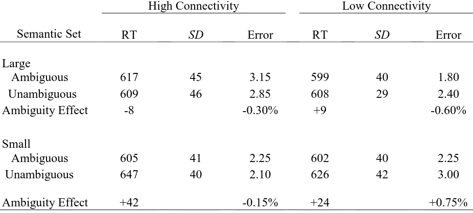
The results from Experiment 1 failed to produce an overall advantage for ambiguous

words over their unambiguous counterparts, although, as in the Locker et al. (2003) experiment,

it did produce a three-way interaction between ambiguity, set size, and connectivity. This

interaction, however, was not the same interaction Locker et al. reported. Locker et al. found an

ambiguity advantage for words with small semantic set sizes and low connectivity. Such was not

the case in the present experiment, in which the ambiguous words in this condition were

processed about 9 ms slower than the unambiguous words. Instead, in the present experiment, no

(28)

connectivity condition produced an ambiguity disadvantage. What should be noted, of course, is

that, according to Locker et al.’s analysis, this condition is the most likely to produce an

ambiguity disadvantage due to the strong activation of neighbors that should arise for those

words. That is, in cases when the scope of semantic activation is very high, as in when words

have large, highly interconnected neighborhoods, there would be greater competition at the

semantic level, which would potentially result in inhibition. The results of Experiment 1 are,

therefore, at least somewhat consistent with Locker et al.’s notions.

What, of course, is somewhat surprising is that there was no ambiguity advantage in any

condition, a result that appears to contradict a long line of research (e.g., Hino & Lupker, 1996;

Kellas et al., 1988; Millis & Button, 1989; Pexman, Hino, & Lupker, 2004; Pexman & Lupker,

1999) and a result that is also inconsistent with the means for all the stimuli used here based on

the ELP database. Specifically, there were large ambiguity advantages in the small set size, high

connectivity (42 ms) and small set size, low connectivity (24 ms) conditions (with the latter one

being the one in which Locker et al. found an ambiguity advantage). The former of these

conditions did show some evidence of an ambiguity advantage in the RT (10 ms) and in the error

(1.63%) analyses, while the latter, as noted, did not. Equally importantly, the one cell with a

significant ambiguity effect in the present experiment, the large set size, high connectivity

condition, showed only a small (8 ms) ambiguity disadvantage in the ELP database, in contrast

to the 28 ms difference reported here.

In an effort to examine the data patterns more fully, separate analyses were done of the

stimuli Locker et al. (2003) used and the ones added for Experiment 1. For the stimuli derived

from Locker et al., mean RTs and error percentages can be found in Table 7. As noted, mean

(29)

new stimuli, mean RTs and error rates can be found in Table 8. For reference, Table 9 contains

the means from the ELP database for the new stimuli.

Analysis of Locker et al.’s (2003) Stimuli

For data from the stimuli used by Locker et al. (2003), the main effect of set size was

significant in the subject analysis, F1(1, 41) = 7.12, p < .05, but not in the item analysis, F2(1, 67)

= 2.59, p < .15, as words with large set sizes had faster latencies than words with small set sizes.

None of the other main effects were significant. A two-way interaction between set size and

connectivity was significant in the subject analysis, F1(1, 41) = 9.53, p < .004, but was not in the

item analysis, F2(1, 67) < 1, p > .30. Most importantly, the three-way interaction between

ambiguity, set size, and connectivity was significant in both analyses, F1(1, 41) = 12.67, p = .001,

F2(1, 67) = 4.93, p < .05.

A simple main effects analysis found that ambiguous words with small set sizes and low

connectivity (M = 637) were processed more slowly than their unambiguous counterparts (M =

614) in the subject analysis, F1(1, 41) = 7.13, p < .05, and this difference was marginally

significant in the item analysis, F2(1, 67) = 2.75, p = .10. This contrast is, of course, the one

contrast in which Locker et al. (2003) found a significant ambiguity advantage. Finally, the

contrast between ambiguous words with small set sizes and high connectivity (M = 628) and

their unambiguous counterparts (M = 650) was significant in the subject analysis, F1(1, 41) =

4.18, p < .05, but not in item analysis, F(1, 67) = 1.97, p < .20. As in the overall data set, there

was an ambiguity disadvantage in the large semantic set size, high connectivity condition,

however, this 14 ms effect was not significant in either analysis, F1(1, 41) = 2.43, p < .15 , F2 < 1.

The error analysis produced no significant effect of set size in the subject analysis, F1(1,

(30)

67) = 2.91, p < .10, with large set size words producing marginally fewer errors than small set

size words. A two-way interaction between ambiguity and set size was significant in the subject

analysis, F1(1, 41) = 4.33, p < .05, but not in the item analysis, F2(1, 67) = 1.46, p < .30. A

two-way interaction between ambiguity and connectivity was marginally significant in the subject

analysis, F1(1, 41) = 3.08, p < .10, and was statistically significant in the item analysis, F(1, 67)

= 6.25, p < .05.

A simple main effects analysis showed that ambiguous words with small set sizes and

high connectivity (M = 1.85%) produced significantly fewer errors than unambiguous words

with small set sizes and high connectivity (M = 5.00%) in both analyses F1(1, 41) = 4.90, p < .05,

F2(1, 67) = 5.87, p < .05. No other differences reached significance (all FS < 2.5).

Analysis of the Added Stimuli

For data from the new stimuli, the main effect of ambiguity was significant in the subject

analysis, F1(1, 41) = 4.07, p = .05, but not in the item analysis F2(1, 69) = 1.07, p > .30, as

unambiguous words were responded to slightly faster than ambiguous words. No other main

effect approached significance. A two-way interaction between ambiguity and set size was

significant in the subject analysis, F1(1, 41) = 4.37, p < .05, and approached significance in the

item analysis F2(1, 69) = 3.05, p < .10. A two-way interaction between ambiguity and

connectivity was also found to be significant in the subject analysis, F1(1, 41) = 10.32, p < .005,

and approached significance in the item analysis F2(1, 69) = 3.29, p < .10. Finally, the three-way

interaction between ambiguity, connectivity, and semantic set size was significant in the subject

analysis, but was not in the item analysis, F1(1, 41) = 4.14, p < .05, F2(1, 69) = 1.04, p > .15.

A simple main effects analysis showed that ambiguous words with large semantic set

(31)

unambiguous counterparts (M = 613) in both analyses, F1(1, 41) = 15.87, p < .001, F2(1, 69) =

7.78, p < .01. No other differences reached significance (all Fs < 1.0).

In the error analysis, the main effect of ambiguity was significant in the subject analysis,

F1(1, 41) = 5.35, p < .05, and approached significance in the item analysis, F2(1, 69) = 3.31, p

< .10, as ambiguous words produced fewer errors than unambiguous words. The main effect of

connectivity was significant in both analyses, F1(1, 41) = 5.77, p < .05, F2(1, 69) = 5.20, p < .05,

as words with low connectivity produced fewer errors than words with high connectivity. The

two-way interaction between ambiguity and set size approached significance in the subject

analysis, F1(1, 41) = 3.09, p < .10, but not in the item analysis, F2(1, 69) = 2.44, p < .15. The

two-way interaction between ambiguity and connectivity was significant in the subject analysis,

F1(1, 41) = 4.59, p < .05, and approached significance in the item analysis, F2(1, 69) = 3.74, p

< .10.

A simple main effects analysis showed that with small set sizes and high connectivity,

ambiguous words (M = 1.43%) produced significantly fewer errors than unambiguous words (M

= 5.48%) in both analyses, F1(1, 41) = 15.57, p < .001, F2(1, 69) = 8.80, p < .005. No other

differences reached significance (all Fs < 1.5).

Experiment 1: Overall

From this examination of this data, several notable patterns emerge. First, the results from

this experiment consistently showed that ambiguous words in the large set size, high connectivity

condition were responded to more slowly than their unambiguous counterparts. Virtually all of

the analyses showed this pattern to some degree. Second, whereas Locker et al. (2003) reported

that the ambiguity advantage only manifested itself in the small set size, low connectivity

(32)

conclusion. Instead, the one condition that most consistently produced at least some hint of an

ambiguity advantage both in the experimental data and in the ELP database (in terms of both

latency and error rates) was the small set size, high connectivity condition.

These results suggest that although the explanation put forth by Locker et al. (2003) may

have some grain of truth to it, it is far from accurate. Locker et al. argued that the processing of

ambiguous words would benefit the most when the scope of activation of the word’s meanings is

minimized. That is, facilitation of processing is optimized when the scope of activation of a

word’s disparate meanings is low. As a result, they argued that the ambiguity advantage would

be observed for words with weak meaning-level activation, and therefore, the ambiguity

advantage should occur in the small set, low connectivity condition. However, Experiment 1

found an ambiguity disadvantage in this condition, and the effect was, in fact, strongest with

Locker’s own stimuli. Second, as was stated previously, the ELP database consistently showed

the strongest ambiguity advantage in the small set size, high connectivity condition, rather than

the small set size, low connectivity condition.

Where Locker et al.’s (2003) analysis was somewhat successful was in the large set size,

high connectivity condition data. This analysis suggested that stronger semantic activation may

result in more competition during processing. Because this condition showed clear evidence of

an ambiguity disadvantage, that result from Experiment 1 provides at least some support for

Locker et al.’s position. That is, the strong inhibitory effect in the large semantic set size, high

connectivity condition is what one could predict if we assumed that the semantic-level

competition was strong enough to nullify any beneficial effect of ambiguity. This result also

bears some similarities to the results of Mirman and colleagues’ (Chen & Mirman, 2012;

(33)

near neighbors, and a facilitory effect of having many distant neighbors. While the methods of

defining and measuring semantic neighbors differ between this study and theirs, it is not

impossible that Mirman and colleagues’ findings reflect a principle that applies essentially

independently of how semantic neighborhood density is measured.

Number of Meanings and Number of Senses Analysis

Before proceeding, one issue that should be addressed is whether the effects observed in

Experiment 1 can be explained in terms of differences in the number of meanings or number of

senses of the ambiguous words that we used. Paralleling what was done by Locker et al. (2003)

in selecting their stimuli, we did not attempt to determine whether the numbers of polysemes and

homonyms were equated across conditions. Thus, it is possible that there were differences along

these lines. To address this issue, data on the number of meanings (NOM) and number of senses

(NOS) of each word used in this experiment were acquired using entries in the Online

Wordsmyth English Dictionary-Thesaurus (Parks, Ray, & Bland, 1998), just as Rodd et al. did.

The overall NOM and NOS characteristics for all words in Experiment 1 can be found in Table 3.

For reference, the NOM and NOS characteristics for the words that Locker used can be found in

Table 10, and the NOM and NOS characteristics for the new word stimuli can be found in Table

11.

When we compared the number of Wordsmyth entries for ambiguous and unambiguous

words, ambiguous words (M = 1.62) had a significantly greater number of Wordsmyth entries

than unambiguous words (M = 1.08), F(1, 147) = 26.44, p < .001. The only condition in which

ambiguous and unambiguous words did not differ significantly in number of Wordsmyth entries

was the large set size, low connectivity condition, F(1,147) = 2.35, p > .10. Despite not

(34)

words in their number of entries. Furthermore, the number of Wordsmyth entries differed very

little across conditions. The only notable difference was between ambiguous words with low

connectivity, and small versus large sets. Ambiguous words with small set sizes and low

connectivity (M = 1.83) had the highest number of entries of all the conditions.

Ambiguous and unambiguous words also differed significantly in the number of

Wordsmyth senses as well. Ambiguous words (M = 9.89) had a significantly greater number of

Wordsmyth senses than unambiguous words (M = 5.13), F(1, 147) = 38.20, p < .001. There was

also a main effect of semantic set size, F(1, 147) = 5.95, p < .018, as words with large semantic

set sizes (M = 8.44) had significantly more Wordsmyth senses than words with small semantic

set sizes (M = 6.48). Finally, there was a significant main effect of connectivity, F(1, 147) = 5.95,

p < .05, as words with low connectivity (M = 8.36) had a significantly greater number of

Wordsmyth senses than words with high connectivity (M = 6.58).

Although there were differences between the number of senses for large set size words

versus small set size words, and high and low connectivity words, these differences could not

explain the present results, as they went in the wrong direction. It is very apparent that having a

greater number of senses did not produce any significant benefit for the ambiguous words in the

large set size, low connectivity condition, or the small set size, low connectivity condition

(which had the greatest number of senses of any condition in this experiment). This analysis

suggests that there are other factors at work that led to the ambiguity disadvantage in the large

set, high connectivity condition than differences in number of meanings and number of senses.

Experiment 2

From the first experiment and the ELP database, it appears that, if there is an ambiguity

(35)

and the interconnectivity of its neighbors is high. Conversely, the condition in which the target

has a large semantic neighborhood and high connectivity, a situation in which representations

would be most likely to compete with one another, we find the best evidence of an ambiguity

disadvantage. These results do, however, raise a couple of questions. First, why was there so

little evidence of any ambiguity advantage? That is, while the ELP database showed a sizable

ambiguity advantage in the small set size condition with the stimuli used in Experiment 1,

Experiment 1 still did not produce any noticeable differences between ambiguous and

unambiguous words in these conditions. Before investing too much in a theoretical interpretation

of the present data, it would seem to be a good idea to search again for the condition(s)

producing the classic ambiguity advantage. A second question is why there was a clear

ambiguity disadvantage in one condition when there is virtually no evidence of such an effect in

the literature? It would, therefore, be important to attempt to replicate the ambiguity

disadvantage that was found in the large set size, high connectivity condition.

One clear weakness of Experiment 1 was that, following Locker et al. (2003), the

maximum cutoff criterion for small set words (14) was very close to the minimum cutoff

criterion for the large set size words (15). Likewise, the distinction between high and low

connectivity words was also somewhat minimal, meaning that neither manipulation was as

strong as it could have been. That is, the problem is that both groups would then contain words

with semantic neighborhood characteristics similar to words in the other group. For example, the

minimum cutoff point for high connectivity was 1.5, whereas low connectivity words had a

maximum cutoff of 1.5. As a result, under these criteria, a word with a set size of 14 and a

connectivity of 1.49 could be included as a small set size, low connectivity word, whereas a

(36)

size, high connectivity condition. While most words in the two groups were not this close to each

other, it is still clear that both manipulations could have been stronger. Thus, Experiment 2 was

an attempt to re-examine the central issues here with new participants, items, and a stronger

manipulation of set size.

Whereas Experiment 1 included semantic ambiguity, semantic set size, and connectivity

as independent variables, the results of Experiment 1, as well as the results from the ELP

database, suggest that the facilitation and inhibition based on ambiguous words is likely to be

strongest in the high connectivity condition, contrary to the previous findings reported by Locker

et al. (2003). The primary focus of this experiment was, therefore, high connectivity words. As a

result, connectivity was discarded as an independent variable, and was instead held constant, so

that all stimuli in Experiment 2 had high connectivity. If large, highly interconnected

neighborhoods are more detrimental to the processing of ambiguous words, there should be an

ambiguity disadvantage in the large set size condition. Further, if an ambiguity advantage were

to arise, the results of Experiment 1 suggest that it should be in the condition with small set sizes.

Method

Participants. Participants were 95 undergraduate psychology students at the University

of Western Ontario, who participated in the study for course credit. The data from 25 participants

were excluded from the experiment on the basis of excessive error rates (>15% for word stimuli,

or >20% for nonword stimuli). Thus, the analyses reported are based on the data from 70

participants. All participants had normal or corrected-to-normal vision, and all were native

English speakers.

Stimuli. The stimuli were four sets of 25 words formed by crossing ambiguity

(37)

the stimuli can be found in the University of South Florida Word Association, Rhyme, and Word

Fragment Norms (Nelson et al., 1998). Words with a number of associates greater than 15 were

classified as having large set sizes (M = 20.46), and words with a number of associates less than

12 were classified as having small set sizes (M = 9.52). All stimuli had a connectivity of at least

1.30 (M = 2.05). All word types were equated in terms of length, CELEX frequency (Baayen,

Piepenbrock, & Gulikers, 1995), orthographic neighborhood size, and concreteness using the

MRC psycholinguistic database (Coltheart, 2007). As in Experiment 1, AoAs of all the word

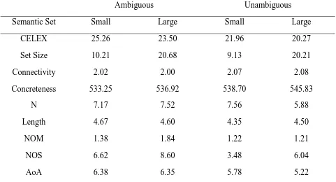
stimuli were collected using the Kuperman et al. (2012) norms. The stimulus characteristics are

shown in Table 12. The stimuli are shown in Appendix B. In addition, 100 orthographically legal

nonwords were used, which were equated with the target words in terms of length and

orthographic neighborhood size. An additional 5 words and 5 nonwords that did not appear in the

experimental trials were presented as practice trials for each participant.

Procedure. The procedure was identical to that used in Experiment 1. Stimulus

presentation and recording of response latencies and accuracy were controlled by an LG Flatron

W2242TQ-BF LCD monitor using DMDX software (Forster & Forster, 2003). At the beginning

of each trial, a fixation stimulus (#####) appeared in the middle of the screen for 750 ms. The

fixation stimulus was then removed, and a word or nonword was presented in uppercase letters.

The target remained on the screen until the participant responded. Lexical decisions were made

by pressing the / key for words and the z key for nonwords. Presentation of trials was

randomized for each participant.

Results and Discussion

Mean lexical decision latencies and error rates for both participants and items were

The Effects of Semantic Neighborhood Density on the Processing of Ambiguous Words