Modified Graph Based Representation of
Multiview Images & Coding
Vandana C A1, Deepa M S2
PG Student [Signal Processing], Dept. of ECE, College of Engineering, Kallooppara, Kerala, India1
Assistant Professor, Dept. of ECE, College of Engineering, Kallooppara, Kerala, India2
ABSTRACT: In this paper, we propose a new geometry representation method for multiview image sets. Our approach relies on graphs to describe the multiview geometry information in a compact and controllable way. The links of the graph connect pixels in different images and describe the proximity between pixels in 3D space. These connections are dependent on the geometry of the scene and provide the right amount of information that is necessary for coding and reconstructing multiple views. Our multiview image representation is very compact and adapts the transmitted geometry information as a function of the complexity of the prediction performed at the decoder side. To achieve this, our graph-based representation (GBR) carefully selects the amount of geometry information needed before coding. Experimental results demonstrate the potential of this new representation. the PWS images is compressed using suitable graph Fourier transforms (GFTs) by considering both the sparsity of the signal’s transform coefficients and the compactness of transform description. Unlike fixed transforms, such as the discrete cosine transform, we can adapt GFT to a particular class of pixel blocks. In particular, a defined search space of GFTs is selected to minimize total representation cost via our proposed algorithms, leveraging on graph optimization techniques, such as spectral clustering and minimum graph cuts..
KEYWORDS: Multiview image coding, 3D representation, view prediction, graph-based representation.
I.INTRODUCTION
MULTIVIEW image processing received considerable attention in recent years. One of the main open questions in multiview image processing is the design of representation methods for multiview data ,where the challenge is to describe the scene content in a compact form that is robust to lossy data compression. All these representations contain two types of data: i) the color or luminance information, which is describes by 2D images; ii) the geometry information that describes the scene’s 3D characteristics, represented by 3D coordinates, depth maps or disparity vectors.For Effective representation, coding and processing of multiview data partly relies on the proper manipulation of the geometry information
The multiview plus depth (MVD) [6] format has become very popular in recent years for 3D data representation and coding. Depth information can be used to build a reliable estimation of scene geometry, enabling encoders to extract the correlations between views [7] and decoders to synthesize virtual views.. However, the representation of geometry with depth maps has one main drawback: if lossy compression is applied to depth images, as done in classical coders, the resulting error affects the quality of synthesized images. This is the case even if the depth gives a good estimation of the 3D scene geometry. More specifically, an error ∆ in the depth value for a first viewpoint (due to quantization for example) leads to a spatial error ∆ when determining the position of the corresponding pixels in neighboring views..
Specifically, we propose a new Graph-Based Representation (GBR) for geometry information, where the geometry of the scene is represented as the connections between corresponding pixels in different views. In this representation, two connected pixels represent neighboring points in the 3D scene. The graph connections are derived from the dense disparity maps and it provide just enough geometry information to predict pixels in all the views that have to be synthesized. GBR drastically simplifies the geometry information to the bare minimum required for view prediction.
directions. Hence, the resulting representation describes 3D points of the scene i.e., the first time they are captured by one of the cameras, and links them through the different views in the graph. And finally 3D images reconstructed
we propose to compress the 3D images using suitable graph Fourier transforms (GFTs) to minimize the total signal representation cost of each pixel block, considering both the sparsity of the signal’s transform coefficients and the compactness of transform description. we design two techniques to reduce computation complexity. In the first technique, we propose a multi-resolution (MR) approach, where detected object boundaries are encoded in the original high resolution (HR), and smooth surfaces are low-passfiltered and down-sampled to a low-resolution (LR) one, before performing LR GFT for a sparse transform domain representation. At the decoder, after recovering the LR block via inverse GFT, we perform up-sampling and interpolation adaptively along the encoded HR boundaries, so that sharp object boundaries are well preserved. The key insight is that on average PWS signals suffer very little energy loss during edge-adaptive low-pass filtering, which enables the low-pass filtering and down-sampling of PWS images. This MR technique also enables us to perform GFT on large blocks, resulting in large coding gain. In the second technique, instead of computing GFT from a graph in real-time via eigen-decomposition of the graph Laplacian matrix, we pre-compute and store the most popular LR-GFTs in a table for simple lookup during actual encoding and decoding. Further, we exploit graph isomorphism to reduce the number of GFTs required for storage to a manageable size.
II.LITERATURE SURVEY
Depth-based representations in multiview image coding suffer from geometry inaccuracies due to lossy compression of depth information, which poses problems in both view prediction quality and compression performance. Different approaches have been proposed recently to improve overall performance while using lossy compression of depth information
Closest to our proposed GBR, several methods have been proposed to reduce redundancy in the geometry representations for multiview data. As an example, the layered depth image (LDI) representation [1], [2] avoids the inter-view redundancies, so that the 3D points of the scene are represented once and only once, in contrast to light field, multiview or depth-based representations, but similar to our proposed approach. In LDI, pixels of multiple viewpoints are projected onto a single view, the redundant pixels are discarded and the new ones (i.e., the ones occluded on this reference view) are added in an additional layer. The main drawback of LDI is that, unlike our method, it directly uses depth, associated to each of the layers. Thus, even if the geometry information is less redundant in LDI, the problem of controlling the error due to depth compression is still present, i.e., no solution is provided to adapt the accuracy of the lossy depth representation to the view synthesis task
III.PROPOSED METHOD
A. Multiview Image Data
We describe now our new Graph-Based Representation approach in detail. We consider a scene captured by N
cameras with the same resolution and focal length f . The n-th view is denoted by , with 1 ≤ n ≤ N, where (r, c) is the pixel at row r and column c. We consider translation between cameras, and we assume that the views are rectified. In other words, the geometrical correspondence between the views only has horizontal components.We also work under the Lambertian assumption, which states that each 3D point of the scene has the same lighting condition when viewed from every possible viewpoint.We assume that a depth image, is available at the encoder for every viewpoint, . Since the views are rectified, the relation between the depth z and the disparity d for two camera views is given by
= (1)
where δ is the distance between the two cameras. In what follows, the geometry information is given by disparity values that are computed from the depth maps and the camera parameters.
B. Geometrical Structure in Multiview Images
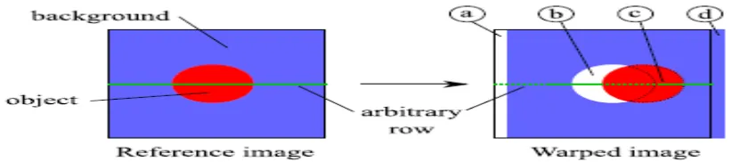
takes the form of ( , ) = ( , + ) ,where d is a disparity value. These correspond to the elements of the scene that are visible in both views. Alternatively, the elements that are visible only from one viewpoint are designed under the general name of occlusions, even if their occurrence is not only due to object occlusions. More exactly, we can categorize these pixels that are present only in one view, into four different types as illustrated in Fig. 2. First, a new part of the scene appears in the view because of camera translation. This usually appears from the right or left (depending on translation direction) and the new pixels are not related to object occlusions. They are called appearing
pixels. During camera translation, foreground objects move faster than the background. As a result, some background pixels may appear behind objects and are thus called disoccluded pixels. Conversely, some background pixels may become hidden by a foreground object. These are called the occluded pixels. Finally, some pixels disappear in the viewpoint change, and they are called disappearing pixels.
Fig. 1. Illustration of camera translation for a simple scene with a uniform background, and one foreground object. Types of pixels in depth-based interview image warping: pixels can be a) appearing, b) disoccluded, c) occluded and d)
disappearing. The green plain line is an arbitrary row in the reference view and the dashed line is the corresponding row in the target view
C. Graph Construction from depth
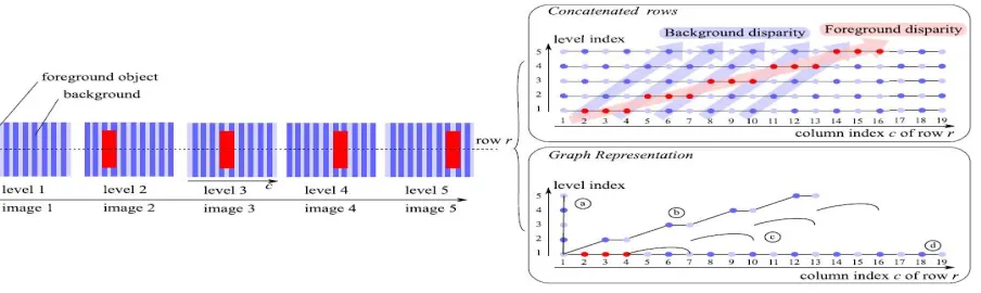
A graph with N levels describes 1 reference view and N −1 predicted views and is constructed based on the depth maps
, 1 ≤n ≤N −1. More precisely, the depth maps are converted to integer disparity values , 1 ≤n ≤N –1.Disparity calculation can be done by comparing the consecutive views and disparity map is plotted .This process continues until the last view.That is we have to compare first and second view ,then second and third,and thus continues. Since the object displacement is only horizontal in our setup with rectified views, the considered graph is constructed independently for each image row. For each row r , the graph incorporates color and geometry components, which are described by two matrices (of size N ×W) and (of size NW × NW), where N is the number of levels (i.e., the number of views encoded by the graph) and W is the image width in pixels. The color values in row r are given by . The matrix is a connectivity matrix between the NW pixels (the ordering of the NW is done from left to right in the view order, i.e., the pixels of the first view are indexed from 1 to W, those of the second view from W+1 to 2W, etc.). A
connection between a pixel i and a pixel j is represented by (i, j ) = 1. In the graph construction, both the color and connectivity matrices are initialized to 0, which means “no connection” and “no color value,” respectively.
We now describe in detail the construction of the graph. We show in Fig. 3 a graph construction example, with 5 levels that correspond to 1 reference view and 4 synthesized views. For the sake of clarity, we first describe in detail the graph construction of an arbitrary row r by considering only one predicted view , one reference view and its associated disparity map . The first level corresponds to the reference view, and thus (1, j ) = (r, j ) for all j ≤W. Then, the connection values (i, j ) and the color values (2, j ) are computed based on the following principles:
The pixels intensities are represented in the graph level (i.e., view) where they appear first, which means that the second level only contains new pixels that are not presentin the reference view.
would have been visible in the previous views, near the other background pixels. The “neighbor” of this new pixel in the lower level l −1 is thus the pixel that is right next to the disoccluded area.
Fig 2. Graph construction example: the blue texture background has a disparity of 1 at each view and the red rectangle foreground has a disparity of 3 for each view. This example graph contains all different types of pixels: a) appearing, b)
disoccluded, c) occluded and d) disappearing
ALGORITHMS
Algorithm 1
GBR Construction for Two Levels Input:
1: { I1 , I2 } – luminance images of height H and width W 2: Z1 – the depth map corresponding to view 1
3: δ – the distance between two views
Output: The color and geometry matrices Γ and Λ
Algorithm:
//Convert depth Z1 to dense disparity map D with rounding operation. 4: for r=1 to H and c=1 to W do
5: ( , ) = [
( , )+ 0.5]
6: end for
7: for r=1 to H do
// Insert I1 in the first level of color matrix Γ
8: for c 1 to W do 9: Γ(r,c,1) I1(r,c) 10: end for
// Insert the D(r,1) appearing pixel in the second level of color matrix Γ
11: for c= 1 to D(r,1) do 12: Γ(r,c,2) I2(r,c)
13: end for
//Link the last appearing pixel to the first pixel of level 1 14: Λ(r,W+D(r,1),1) 1
15: c1 2 // current column index in I1 16: dp D(r,1) // previous disparity value
17: cstop D(r,c1)+1 // column index in level 2 that serves as stopping criterion 18: while cstop ≤ W do
19: dc D(r,c1) // current disparity value
21: ∆disp = dc - dp
//test if ∆disp corresponds to a disocclusion ( > 0 ) or an occlusion (< 0 )
22: if ∆disp> 0 then
23: cstop cstop+ ∆disp
// Fill the disoccluded pixels in second level of Γ
24: for c2 c1+dp to min(c1+dp+∆disp -1,W) do 25: Γ(r,c,2) I2(r,c2)
26: end for
// Include the link between the two neighbours in the 3D space in Λ 27: Λ ( r , c1-1 , c1+dp+W ) 1
28: else
// Deal with Occlusion Manager using algorithm 2
29: ( Λ, Γ ) Occlusion Manager ( c1 , c2 , dp , D , Γ , Λ , I2 ) 30: end if
31: else
32: cstop cstop +1 33: end if
34: dp dc 35: c1 c1+1 36: end while
37: end for
Algorithm 2 - Occlusion Manager
Input :
1: c1 , c2 , dp , D , Γ , Λ , I2
Output : The color and geometry matrices Γ and Λ
Algorithm:
// The last pixel of the foreground object 2: clast c1
// The pixel to link with clast and determined in the loop from line 6 to 18 3: ctemp c1
// Disparity value of clast 4: dtemp dp
5: stop=0
// The loop is looking for the pixel linked with clast after the occlusion ,a disocclusion may appear 6: while stop=0 do
7:ctemp ctemp +1 8: dtemp dtemp-1 9: dcur D( r,ctemp,1) // If a disocclusion appears 10: if dtemp ≠ dcur then // size of disocclusion 11: Ndisoc =dcur –dtemp -1
// Handle the disocclusion as in Algorithm 1 lines 22 to 28 12: for c2 clast+dp+1 to min(clast +dp+Ndisoc ,W) do 13: : Γ(r,c2,2) I2(r,c2)
14: end for
15 : Λ ( r , clast , clast+dp+W ) 1
18: end while
// Link the last pixel of the foreground clast to the first pixel after the occlusion ctemp determined by the lines 6 to 18
19: : Λ ( r , clast , ctemp) 1
20:
[1]
GBR view reconstruction and synthesis View Reconstruction From GBR
The reconstruction of a certain view requires the color values and the connections of all lower levels. The reconstruction of the color values in the current view is performed by navigating the graph across its different levels. This navigation starts from the border of the image at the level (i.e., view) that needs to be constructed; it then follows the connections and refers to the lower levels when no color information is available at current level. an example of a view synthesis for the image of level 2, based on the graph in the example of Fig. 3. The pixel numbering is done with respect to the column index of as in Fig. 3. The reconstruction starts with the appearing pixel 1 at level 2. Then, it moves to the reference level and fills pixel color values until encountering a non-zero connection. The first connection is after pixel 2 and links it to pixel 3 and 4 in level 2. After filling all the disoccluded pixels, the reconstruction goes back to the reference level and fills color information (5, 6 and 7) until the next non-zero connection (at pixel 7). The connection in 7 indicates an occluded region. Hence, the reconstruction algorithm jumps across columns in the reference view and continues the decoding of the pixels in the reference level for pixel 8 to 19 until it recovers the entire row. The reconstruction of the other views (i.e., the other levels of the graph in multiview images) is done recursively
Algorithm 3
Input:
1.The graph connections Λ for row r
Output:
The disparity map D for row r
Algorithm:
2: D(r,1) number of appearing pixel 3: dtemp D(r,1)
4: for c:=1 to W do
5 :if Ǝ j such as Λ(r,c,j) indicates a disocclusion then 6: dtemp dtemp+ number of disoccluded pixel 7: D(r,1) dtemp
8: end if
9: if Ǝ j such as Λ(r,c,j) indicates a occlusion then 10: dtemp dtemp-number of disoccluded pixel 11: D(r,1) dtemp
12: end if 13: end for
Multiresolution Graph Fourier Transform For Compression Of Piecewise Smooth Images
We first provide an overview of our proposed MR-GFT coding system for compression of 3D images, obtained from GBR view reconstruction Given a PWS image, we discuss the encoding and decoding procedures as follows.
A. Encoder
First, we perform aware intra prediction as proposed. Different from the intra prediction in H.264, edge-aware intra prediction efficiently reduces the energy of the prediction error by predicting within the confine of detected HR boundaries, thus reducing bits required for coding of the residual signal.
Second, we try two types of transforms for transform coding of the residual block: i) fixed DCT on the original HR residual block (HR-DCT), ii) a pre-computed set of LR GFT (LR-GFT) on the down-sampled LR residual block (including LR weighted GFT and LR unweighted GFT, as discussed in Section V). We then choose the one transform with the best RD performance. Before transform coding using LR-GFT, however, we first adaptively low-pass-filter and down-sample the K√N × K√N block uniformly to a√N ×√N block. Low-pass filtering is first used to avoid aliasing caused bydown-sampling. We propose an edge-adaptive low-pass filterin the pixel domain for the preservation of sharp boundaries.Specifically, a pixel is low-pass-filtered by taking average ofits neighbors on the same side of HR boundaries within a(2K − 1) × (2K − 1) window centering at the to-be-filteredpixel. The advantage of this edge-adaptive low-pass filteringis that filtering across arbitrary-shape boundaries will not occur, so pixels across boundaries will not contaminate eachother through filtering.
For the implementation of the HR-DCT and LR-GFT, we pre-compute the optimal transforms and store them in a lookup table a priori. During coding, we try each one and choose the one with the best RD performance. The two types of transforms, HR-DCT and LR-GFT, are employed to adapt to different block characteristics.HR-DCT is suitable for blocks where edge-adaptive low-pass filtering would result in non-negligible energy loss. If very little energy is lost during low-pass filtering, LR-GFT would result in a larger coding gain. Note that if a given block is smooth, the LR-GFT will default to the DCT in LR, and would generally result in a larger gain than HR-DCT due to down-sampling (the rates of transform indices for both, i.e., the transform description overhead, are the same in this case).
Third, after the RD-optimal transform is chosen from the two transform candidates, we quantize and entropy-encode the resulting transform coefficients for transmission to the decoder. The transform index identifying the chosen transform is also encoded, so that proper inverse transform can be performed at the decoder.
B. Decoder
At the decoder, we first perform inverse quantization and inverse transform for the reconstruction of the residual block. The transform index is used to identify the transform chosen at the encoder for transform coding. Secondly, if LR-GFT is employed, we up-sample the reconstructed √N×√N LR residual block to the original resolutionK√N×K√N, and then fill in missing pixels via our proposedimage-based edge-adaptive interpolation , where a pixel x is interpolated by taking average of its neighboring pixels on the same side of boundaries within a (2K − 1) ×
(2K − 1) window centering at pixel x. Finally, the K√N×K√N block is reconstructed by adding the intrapredictor to the residual block.
IV. RESULT AND DISCUSSION
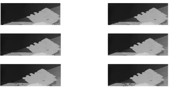
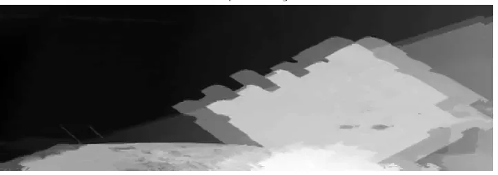
Different views of input depth images of Statue dataset is shown below
By applying Graph Based Representation we obtain color value and connection value as output. the color or luminance information, which is describes by 2D characteristics of the images; the connection value represents geometry information that describes the scene’s 3D characteristics,
Fig. 4. Six different views synthesized from GBR
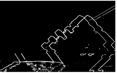
3D images can be reconstructed from the graph based representation using the reconstructon algorithm.which is shown in fig 5
Fig 5. Reconstructed 3D Image
We exthact prominent boundaries (large inter-pixel intensity difference) in the HR image via hard thresholding of image gradients.
we perform edge-aware intra prediction as proposed. Different from the intra prediction in H.264, edge-aware intra prediction efficiently reduces the energy of the prediction error by predicting within the confine of detected HR boundaries, thus reducing bits required for coding of the residual signal
Fig 7 Intra prediction during encoding
We perform inverse quantization and inverse transform for the reconstruction of the residual block and prominant edges are detected
Fig 8 Edges during decompression
We perform inverse quantization and inverse transform for the reconstruction of the residual block Finally, the K√N×K√N block is reconstructed by adding the intrapredictor to the residual block to obtain the decompressed image
Fig 9 Decompressed image intra prediction
edges
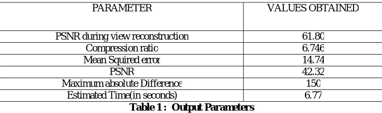
PARAMETER VALUES OBTAINED
PSNR during view reconstruction 61.80
Compression ratio 6.746
Mean Squired error 14.74
PSNR 42.32
Maximum absolute Difference 150
Estimated Time(in seconds) 6.77
Table 1 : Output Parameters
.V. CONCLUSION
In this project an alternative method to depth for multiview geometry representation is proposed . Using graphs to describe connections between pixels of different views, our method represents the true geometry in the scene and avoids the inter-view redundancies. Obtained two matrices as output of Graph based representation , color and connection matrices.and also obtained the multiple views during reconstruction and a concatenated images of multiple views. The links of the graph connect pixels in different images and describe the proximity between pixels in 3D space. These connections are dependent on the geometry of the scene and provide the right amount of information that is necessary for coding and reconstructing multiple views.
Also proposed and implemented an efficient method to compress the PWS images using suitable graph Fourier transforms (GFTs) to minimize the total signal representation cost of each pixel block, considering both the sparsity of the signal’s transform coefficients and the compactness of transform description.
REFERENCES
[1] T. Maugey, A. Ortega, and P. Frossard, “Multiview image graph-based Representation of Multiview images ,” in Proc. IEEE Trans. Image Process., vol. 24, no. 5, pp. 1573-1586,May 2015
[2] A. Gelman, P. L. Dragotti, and V. Velisavljevi´c, “Multiview image coding using depth layers and an optimized bit allocation,” IEEETrans. Image Process., vol. 21, no. 9, pp. 40
[3]U. Takyar, T. Maugey, and P. Frossard , “Extended layered depth image representation
in multiview navigation,” IEEE Signal Process. Lett., vol. 21, no. 1, pp. 22–25, Jan. 201492–4105, Sep. 2012.
[4] F. Maninchedda, M. Pollefeys, and A. Fogel, “Efficient stereo video encoding for mobile applications using the 3D+F codec ,” in Proc. IEEE 3DTV-Conf., Zürich, Switzerland, Oct. 2012, pp. 1–4.
[5]T. Maugey, A. Ortega, and P. Frossard, “Graph-based representation and coding of multiview geometry,” in Proc. IEEE Int. Conf. Acoust., Speech, Signal Process., Vancouver, BC, Canada, May 2013, pp. 1325–1329.
[6] T. Maugey, A. Ortega, and P. Frossard, “Multiview image coding using graph-based approach,” in Proc. IEEE 11th Workshop 3D Image/Video Technol. Appl. (IVMSP), Seoul, Korea, Jun. 2013, pp. 1–4.
[7] P. Merkle, A. Smolic, K. Müller, and T. Wiegand, “Multi-view video plus depth representation and coding,” in Proc. IEEE Int. Conf. Image Process., San Antonio, TX, USA, Sep./Oct. 2007, pp. I-201–I-204.
[8] T. Maugey, Y.-H. Chao, A. Gadde, A. Ortega, and P. Frossard, “Luminance coding in graph-based representation of multiview images,” in Proc. IEEE Int. Conf. Image Process., Paris, France, Oct. 2014, pp. 130–134.
[9] S. Yea and A. Vetro, “View synthesis prediction for multiview video coding,” EURASIP J. Signal Process., Image Commun., vol. 24, nos. 1–2, pp. 89–100, 2009.
[10] K. Müller et al., “3D high-efficiency video coding for multi-view video and depth data,” IEEE Trans. Image Process., vol. 22, no. 9, pp. 3366– 3378, Sep. 2013.
BIOGRAPHY