Developing Decision Trees for Handling
Uncertain Data
P. Satya Prakash, P. Jhansi Lakshmi, B.L Krishna
Department of Computer Science, Vignan University, Vadlamudi (A.P)INDIA
Abstract— Classification is one of the most efficient and widely used data mining technique. In classification, Decision trees can handle high dimensional data, and their representation is intuitive and generally easy to assimilate by humans. Decision trees handle the data whose values are certain. We extend such classifiers i.e, decision trees to handle uncertain information. Value uncertainty arises in many applications during the data collection process. Example sources of uncertainty include data staleness, and multiple repeated measurements. With uncertainty, the value of a data item is often represented not by one single value, but by multiple values forming a probability distribution (pdf’s). Rather than abstracting uncertain data by statistical derivatives (such as mean and median), we extend classical decision tree building algorithms to handle data tuples with uncertain values. Extensive experiments have been conducted that show that the resulting classifiers are more accurate than those using value averages.
Index Terms—Uncertain Data, Decision Tree, Classification, Data Mining
I.INTRODUCTION
In this modern world, huge amount of information is kept in the databases. Thus data-mining can be very effective for extracting knowledge from huge amount of data. Classification has many applications in real world, such as stock planning of large superstores, medical diagnosis, etc. Classification is separation or ordering of objects into classes. There are various classification techniques i.e. Decision tree, K-nearest neighbour, Naïve bayes classifier, neural network. In this paper we discuss decision tree. Classification is a classical problem in machine learning and data mining[1]. It summarizes an approach for synthesizing decision trees that has been used in a variety of systems, and it describes one such system, ID3, in detail. Decision trees are mainly used for handling “Decision-making”. Many algorithms, such as ID3 [2] and C4.5 [3], have been devised for decision tree construction. C4.5 is an extension to ID3 algorithm.
In traditional decision-tree classification, a feature (an attribute) of a tuple is eithercategorical or numerical. For the latter, a precise and definite point value is usually assumed. In many applications, however, data uncertainty is common. The value of a feature/attribute is thus best captured not by a single point value, but by a range of values giving rise to a probability distribution. A simple way to handle data uncertainty is to abstract probability distributions by summary statistics such as means and variances. We call this approach “Averaging”. Another approach is to consider the
complete information carried by the probability distributions to build a decision tree. We call this approach “Distribution-based”. Our goals are (1) to devise an algorithm for building decision trees from uncertain data using the based approach; (2) to investigate whether the Distribution-based approach could lead to a higher classification accuracy compared with the Averaging approach; and (3) to establish a theoretical foundation on which pruning techniques are derived that can significantly improve the computational efficiency of the Distribution-based algorithms.
II.RELATED WORK
Decision trees are one of the most important aspect for “Decision-making”. Classification is one of the most widespread datamining problems found in real life. Decision tree classification is one of the best-known solution approaches. ID3, first proposed by Quinlan is a particularly elegant and instinctive solution [4]. This article presents an algorithm for privately building an ID3 decision tree. While this has been done for horizontally partitioned data [5], Lindell et al has proposed a secure algorithm to build a
III.APPROACHES
There are two approaches for handling uncertain data. The first approach, called “Averaging,” transforms an uncertain data set into a point-valued one by replacing each pdf with its mean value. More specifically, the mean value v,
x f, x dx
,
, as its representative value. The feature vector
of ti is thus transformed to (v, ,………..,v, ) A decision tree can
then be built by applying a traditional tree construction algorithm.
Several identical algorithms have been introduced for decision tree construction. This work provides the ID3 classification algorithm. Very simply, ID3 builds a decision tree from a fixed set of examples. The resulting tree is used to classify future samples. C4.5 is an algorithm used to generate
a decision tree developed by Ross Quinlan. C4.5 is an extension of Quinlan's earlier ID3 algorithm. The decision trees generated by C4.5 can be used for classification, and for this reason, C4.5 is often referred to as a statistical classifier. We present details of the tree construction algorithms under the two approaches in the following sections.
To exploit the full information carried by the pdfs, our second approach, called “Distribution-based,” considers all the sample points that constitute each pdf. The challenge here is that a training tuple can now “pass” a test at a tree node probabilistically when its pdf properly contains the split point of the test.
1.Averaging
A straightforward way to deal with the uncertain information is to replace each pdf with its expected value, thus, effectively converting the data tuples into point-valued tuples. This reduces the problem back to that for point valued data, and hence, traditional decision tree algorithms such as ID3 and C4.5 [3] can be reused. We call this approach Averaging (AVG).
AVG is a greedy algorithm that builds a tree top-down. When processing a node, we examine a set of tuples S. The algorithm starts with the root node and with S being the set of all training tuples. At each node n, we first check if all the tuples in S have the same class label c. If so, we make n a leaf node and set 1, 0 . Otherwise, we select an attribute A and a split point z and divide the tuples into two subsets: “left” and “right.” All tuples with
v, z are put in the “left” subset L; the rest goes to the
“right” subset R. If either L or R is empty (even after exhausting all possible choices of A and z ), it is impossible to use the available attributes to further discern the tuples in S. In that case, we make n a leaf node. Moreover, the population of the tuples in S for each class label induces the probability distribution . In particular, for each class label c C, we assign to Pn(c) the fraction of tuples in S that is labeled c. If neither L nor R is empty, we make n an internal node and create child nodes for it. We recursively invoke the algorithm on the “left” child and the “right” child, passing to them the sets L and R,respectively. To build a good decision tree, the choice of A and z is crucial. At this point, we may assume that this selection is performed by a black box algorithm BestSplit, which takes a set of tuples as parameter, and returns the best choice of attribute and split point for those tuples.
one attribute, whose (discrete) probability distribution is shown under the column “probability distribution.” For instance, tuple 3 has class label “A” and its attribute takes the values of -1, +1, +10 with probabilities 5/8, 1/8, 2/8, respectively. The column “mean” shows the expected value of the attribute. For example, tuple 3 has an expected value of +2.0. With Averaging, there is only one way to partition the set: the even-numbered tuples go to L and the odd-numbered tuples go to R. The tuples in each subset have the same mean attribute value, and hence, cannot be discerned further. The resulting decision tree is shown in Fig. 2a. Since the left subset has 2 tuples of class B and 1 tuple of class A, the left leaf node L has the probability distribution (A) =1/3 and (B) =2/3 over the class labels. The probability distribution of class labels in the right leaf node R is determined analogously. Now, if we use the six tuples in Table 1 as test tuples4 and use this decision tree to classify them, we would classify tuples 2,4,6 as class “B” (the most likely class label in L), and hence, misclassify tuple 2. We would classify tuples 1, 3, 5 as class “A,” thus getting the class label of 5 wrong. The accuracy is 2=3.
Fig. 3. Example decision tree before post pruning. Typically, BestSplit is designed to select the attribute and split point that minimize the degree of dispersion. The degree of dispersion can be measured in many ways, such as entropy. We assume that entropy is used as the measure since it is predominantly used for building decision trees. For each of the (m-1)k combinations of attributes (A and split points (z), we divide the set S into the “left” and “right” subsets L and R. We then compute the entropy for each such combination:
H(z,A)=∑ |X| |S|
X L,R ∑ C PC/Xlog PC/X
where PC=X is the fraction of tuples in X that is labeled c.
2. Distribution-Based Approach
For uncertain data, we adopt the same decision tree building framework as described above for handling point data. After an attribute A and a split point z have been chosen for a node n, we have to split the set of tuples S into two subsets L and R. The major difference from the point data case lies in the way the set S is split. Recall that the pdf of a tuple t S under attribute A spans the interval [a, ,b, ]. If b, z ,
the pdf of ti lies completely on the left of the split point, and thus, is assigned to L. Similarly, we assign t to R ifz a, . If the pdf properly contains the split point, i.e., a, z b, , we split ti into two fractional tuples and and add
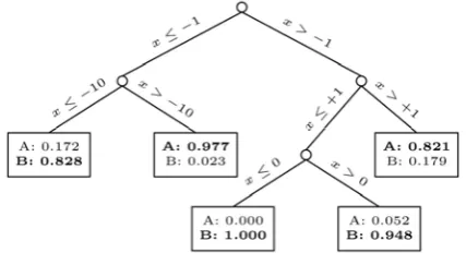
them to L and R, respectively. We call this algorithm Uncertain Decision Tree (UDT). Let us reexamine the example tuples in Table 1 to see how the distribution-based algorithm can improve classification accuracy. By taking into account the probability distribution, UDT builds the tree shown in Fig. 3 before pre pruning and post pruning are applied. This tree is much more elaborate than the tree shown in Fig. 2a because we are using more information, and hence, there are more choices of split points. The tree in Fig. 3 turns out to have a 100 percent classification accuracy. After post pruning, we get the tree in Fig. 2b. Now, let us use the six tuples in Table 1 as testing tuples to test the tree in Fig. 2b. For instance, the classification result of tuple 3 gives P(A)=5/8*0:80 + 3/8 *0:212= 0:5795 and P(B) =5/8*0:20 +3/8 * 0:788 =0:4205. Since the probability for “A” is higher, we conclude that tuple 3 belongs to class “A.” All the other tuples are handled similarly, using the label of the highest probability as the final classification result. It turns out that all six tuples are classified correctly. This handcrafted example thus illustrates that by considering probability distributions rather than just expected values, we can potentially build a more accurate decision tree.
TABLE 2 Selected Data Sets from the UCI Machine Learning Repository
IV.ID3 ALGORITHM
The ID3 algorithm is used to build a decision tree, given a set of non-categorical attributes C1, C2, .., Cn, the categorical attribute C, and a training set T of records.
1) function ID3 (R: a set of non-categorical attributes, C: the categorical attribute,
S: a training set) returns a decision tree; begin
4)If R is empty, then return a single node with as value 5) the most frequent of the values of the categorical attribute that are found in records of S; [note that then there will be errors, that is, records that will be improperly classified]; 6) Let D be the attribute with largest Gain(D,S) among attributes in R;
a)Let {d| j=1,2, .., m} be the values of attribute D; b)Let {s | j=1,2, .., m} be the subsets of S consisting
c)respectively of records with value dfor attribute D; Return a tree with root labeled D and arcs labeled d1, d2, .., dm going respectively to the trees
{D}, C, S1), {D}, C, S2), .., ID3(R-{D}, C, Sm);
end ID3;
V.EXPERIMENTS ON ACCURACY
In order to achieve a higher classification accuracy by considering data uncertainty, we should implement AVG and UDT and apply them to 10 real data sets (see Table 2) taken from the UCI Machine Learning Repository [17]. These data sets are chosen because they mostly contain numerical attributes obtained from the measurements.
Here, first data set contains 640 tuples, each representing an utterance of the Japanese vowels by one of the nine participating speakers. Each tuple contains 12 numerical attributes, which are Linear Predictive Coding (LPC) coefficients. These coefficients reflect important features of speech sound. Each attribute value consists of 7-29 samples of LPC coefficients collected over time. These samples represent uncertain information and are used to model the pdf of the attribute for the tuple.
The other nine data sets contain “point values” without uncertainty.
TABLE 3Accuracy Improvement by Considering the Distribution
We enhance uncertainty information by fitting appropriate error models on to the point data. For each tuple t and for each attribute Aj, the point value v, reported in a data set is
used as the mean of a pdf f,, defined over an interval [ai,j;
bi,j].The range of values for A (over the whole data set) is noted and the width of [a,, b,] is set to w. |A|, where |A|
denotes the width of the range for A and w is a controlled parameter. The results of applying AVG and UDT to the 10
data sets are shown in Table 3. Using C4.5 [3] the information gain is calculated. In the experiments, each pdf is represented by 100 sample points (i.e., s=100), except for the “JapaneseVowel” data set. We have repeated the experiments using various values for w. For most of the data sets, Gaussian distribution is assumed as the error model. Since the data sets “PenDigits,” “Vehicle,” and “Satellite” have integer domains, we suspected that they are highly influenced by quantization noise. So, we have also tried uniform distribution on these three data sets, in addition to Gaussian.6 For the “JapaneseVowel” data set, we use the uncertainty given by the raw data (7-29 samples) to model the pdf.
VI.EFFECT OF NOISE MODEL
In the experiment above, we have taken data from the UCI repository and directly added uncertainty to it so as to test our UDT algorithm. The amount of errors in the data is uncontrolled. So, in the next experiment, we inject some artificial noise into the data in a controlled way except the “JapaneseVowel”. For each tuple t and for each attributeA, the point value v, is perturbed by adding a Gaussian noise
with zero mean and a standard deviation equal to ~=1/4(u. |A|), where u is a controllable parameter. So, the perturbed value is v,= v,+∆,, where ∆, is a random number which
follows N(0,σ ).
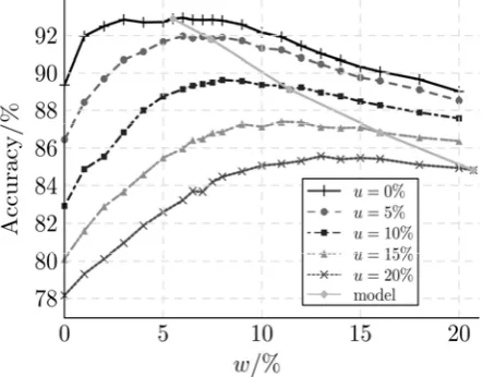
Fig. 4. Experiment with controlled noise on data set “Segment.”
Each curve in the figure corresponds to one value of u, which controls the amount of perturbation that has been artificially added to the UCI data set. The x-axis corresponds to different values of w—the errormodel that we use as the uncertainty information. The y-axis gives the accuracy of the decision tree built by UDT.
VII.PRUNING ALGORITHMS
Pruning Empty and Homogeneous Intervals:
v -1. We will examine each interval separately. For convenience, an interval is denoted by (a,b].
Definition 2 (Empty interval): An interval (a,b] is empty if
f , x dx 0 for all t S.
Definition 3 (Homogeneous interval): An interval (a, b] is homogeneous if there exists a class label c C such that
f , x dx 0 c c for all t S.
Definition 4 (Heterogeneous interval): An interval (a,b] is
heterogeneous if it is neither empty nor homogeneous.
Theorem 1: If an optimal split point falls in an empty
interval, then an end point of the interval is also an optimal split point.
Proof: By the definition of information gain, if the optimal
split point can be found in the interior of an empty interval (a,b], then that split point can be replaced by the end point a without changing the resulting entropy. As a result of this theorem, if (a,b] is empty, we only need to examine the end point a when looking for an optimal split point. There is a well-known analogue for the point data case, which states that if an optimal split point is to be placed between two consecutive attribute values, it can be placed anywhere in the interior of the interval and the entropy will be the same [28]. Therefore, when searching for the optimal split point, there is no need to examine the interior of empty intervals. The following theorem further reduces the search space:
Theorem 2: If an optimal split point falls in a homogeneous
interval, then an end point of the interval is also an optimal split point.
Definition 5 (Tuple density): Given a class c C, an
attribute A, and a set of tuples S, we define the tuple density function g , as
g , w f ,
S:
where w is weight of the fractional tuple S
Definition 6 (Tuple count): For an attributeA, the tuple
count for class c C in an interval (a, b] is
γ , a, b g, x dx
Theorem 3: Suppose that the tuple count for each class
increases linearly in a heterogeneous interval (a, b] (i.e.,
C, t 0,1 ,γ , a, 1 t a tb β t for some constant β ). If an optimal split point falls in ða; b_, then an end point of the interval is also an optimal split point.
VIII.END POINT SAMPLING
UDT-GP Global Pruning algorithm is very effective in pruning intervals. In some settings, UDT-GP reduces the number of “entropy calculations” (including the calculation of entropy values of the split points and the calculation of entropy-like lower bounds for intervals) to only 2.7 percent of that of UDT.
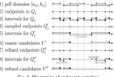
Fig. 5. Illustration of end point sampling.
In fig, Row 1 shows the intervals obtained from the domains of the pdfs. The collection of end points of these intervals constitutes the set Q(row 2). From these end points, disjoint intervals are derived (row 3). Instead of using the set of all end points Q(row 2), we take a sample Q (row 4) of these points. The algorithm thus operates on the intervals derived from Q (row 5) instead of those derived from Q(row 3). After all the pruning’s on the coarser intervals are done, we are left with a set Y 0 of candidate intervals (row 6). (Note that a couple of end points are pruned in the second interval of row 5.) For each unpruned candidate interval q , q in row 6, we bring back the original set of end points inside the interval (row 7) and their original finer intervals (row 8). The candidate set of intervals obtained after pruning is Y (row 9), which is a much smaller candidate than the set of candidate intervals when no end point sampling is used. We incorporate these end point Sampling strategies into UDT-GP. The resulting algorithm is called UDT-ES.
Fig. 5.Effects of s on UDT-ES.
IX.CONCLUSION
accuracy. Several procedures and algorithm handles data uncertainty. We exploit data uncertainty that leads to decision trees with remarkably higher accuracies.
ACKNOWLEDGMENT:
This research is supported by the Vignan University, Andhra Pradesh, India, Asst prof. Mrs P.Jhansi Lakshmi, HOD Mr. K.V. Krishna Kishore.
REFERENCES:
[1] J. R. Quinlan, “Induction of decision trees,” Machine Learning, vol. 1, no. 1, pp. 81–106, 1986.J. R. Quinlan, “Learning logical definitions from relations,” Machine Learning, vol. 5, pp. 239–266, 1990. [2] J. Kinoshita, “Fuzzy decision trees by fuzzy ID3 algorithm and its
application to diagnosis systems,” in Fuzzy Systems, 1994, vol. 3. IEEE World Congress on Computational Intelligence, 26-29 Jun. 1994, pp.2113–2118.
[3] C4.5: Programs for Machine Learning. Morgan Kaufmann, 1993,ISBN 1-55860-238-0.
[4] J.R. Quinlan, “Induction of decision trees,” In Jude W.Shavlik, Thomas G. Dietterich, (Eds.), Readings in Machine Learning. Morgan Kaufmann, 1990. Originally published in Machine Learning, vol. 1, 1986, pp 81–106.
[5] Y. Lindell, B. Pinkas, “Privacy preserving data mining,” In Journal of Cryptology vol. 15, no. 3, 2002, pp 177–206.
[6] M. Chau, R. Cheng, B. Kao, and J. Ng, “Uncertain data mining: An example in clustering location data,” in PAKDD, ser. Lecture Notes in Computer Science, vol. 3918. Singapore: Springer, 9–12 Apr. 2006, pp. 199–204
[7]J. Chen and R. Cheng, “Efficient Evaluation of Imprecise Location- Dependent Queries,” Proc. Int’l Conf. Data Eng. (ICDE), pp. 586- 595, Apr. 2007.
[8] M. Chau, R. Cheng, B. Kao, and J. Ng, “Uncertain Data Mining: An Example in Clustering Location Data,” Proc. Pacific-Asia Conf. Knowledge Discovery and Data Mining (PAKDD), pp. 199-204, Apr. 2006.
[9] W. K. Ngai, B. Kao, C. K. Chui, R. Cheng, M. Chau, and K. Y. Yip, “Efficient clustering of uncertain data,” in ICDM. Hong Kong, China: IEEE Computer Society, 18–22 Dec. 2006, pp. 436–445.
[10] S. D. Lee, B. Kao, and R. Cheng, “Reducing UK-means to K-means,” in The 1st Workshop on Data Mining of Uncertain Data (DUNE), in conjunction with the 7th IEEE International Conference on Data Mining (ICDM), Omaha, NE, USA, 28 Oct. 2007.
[11] T. Elomaa and J. Rousu, “General and Efficient Multisplitting of Numerical Attributes,” Machine Learning, vol. 36, no. 3, pp. 201- 244, 1999.
[12] U.M. Fayyad and K.B. Irani, “On the Handling of Continuous- Valued Attributes in Decision Tree Generation,” Machine Learning, vol. 8, pp. 87-102, 1992.
[13] T. Elomaa and J. Rousu, “Efficient Multi-splitting Revisited: Optima-Preserving Elimination of Partition Candidates,” DataMining and Knowledge Discovery, vol. 8, no. 2, pp. 97 126, 2004.
[14]H.-P. Kriegel and M. Pfeifle, “Density-Based Clustering of Uncertain Data,” Proc. Int’l Conf. Knowledge Discovery and Data Mining (KDD), pp. 672-677, Aug. 2005.
[15] C.K. Chui, B. Kao, and E. Hung, “Mining Frequent Itemsets from Uncertain Data,” Proc. Pacific-Asia Conf. Knowledge Discovery and Data Mining (PAKDD), pp. 47-58, May 2007.
[16] C.C. Aggarwal, “On Density Based Transforms for Uncertain Data Mining,” Proc. Int’l Conf. Data Eng. (ICDE), pp. 866-875, Apr. 2007. [17] A. Asuncion and D. Newman, UCI Machine Learning