Numerical Experiments on Eigenvalues
of Weakly Singular Integral Equations
Using Product Simpson’s Rule
Mohamad Rashidi Razali & Mohamed M. S. Nasser
Department of Mathematics, Faculty of Science
Universiti Teknologi Malaysia
81310 UTM Skudai, Johor, Malaysia
Abstract This paper discusses the use of Product Simpson’s rule to solve the integral equation eigenvalue problem λf(x) = R−11k(|x−y|)f(y)dy where k(t) = ln|t| or k(t) =t−α, 0< α <1, λ, f and are unknowns which we wish to obtain. The functionf(y) in the integral above is replaced by an interpolat-ing function Lfn(y) =
Pn
i=0f(xi)φi(y), where φi(y) are Simpson interpolating
elements andx0, x1, . . . , xn are the interpolating points and they are chosen to
be the appropriate non-uniform mesh points in [−1,1]. The product integra-tion formulaR−11k(y)f(y)dy≈Pin=0wif(xi) is used, where the weightswi are
chosen such that the formula is exact whenf(y) is replaced byLfn(y) andk(y)
as given above. The five eigenvalues with largest moduli of the two kernels K(x, y) = ln|x−y|andK(x, y) =|x−y|−α, 0< α <1 are given.
Keywords eigenvalue, product integration, singular kernel, integral equation.
Abstrak Kertas kerja ini membincangkan penggunaan aturan Simpson darab untuk menyelesaikan masalah nilai eigen persamaan kamiranλf(x) =R−11k(|x−
y|)f(y)dy dengank(t) = ln|t| atauk(t) =t−α, 0< α <1,λdan f adalah anu
yang hendak didapatkan. Fungsi interpolasiLf n(y) =
Pn
i=0f(xi)φi(y), dengan
φi(y) unsur interpolasi Simpson danx0, x1, . . . , xn adalah titik-titik dan ianya
dipilih supaya menjadi titik-titik interpolasi tak seragam yang tertentu dalam
[−1,1]. Rumus pengamiran darabR−11k(y)f(y)dy ≈ Pni=0wif(xi) digunakan
dengan pemberat wi dipilih supaya rumus adalah tepat apabila f(y) diganti
olehLf
n(y)dank(y)seperti di atas. Lima nilai eigen dengan modulus terbesar
bagi kedua-dua inti K(x, y) = ln|x−y| dan K(x, y) = |x−y|−α, 0< α <1
diberikan.
1
Introduction
The numerical solution of the integral equation eigenvalue problem
λf(x) = Z 1
−1
K(x, y)f(y)dy (1)
for an eigenvalue λand a corresponding eigenfunctionf(x) is considered in this paper. If λ is an eigenvalue of the kernel K(x, y), then there is at least one non-null function f(x) satisfying (1). The function f(x) is called a left-eigenfunction or only eigenfunction corre-sponding to the eigenvalueλ. If there exists a functiong(x) such thatλg(x) =R−11K(x, y)dy theng(x) is called the right-eigenfunction corresponding to λ.
In this paper, we shall discuss only when K(x, y) is a weakly singular kernel and has the form
K(x, y) =|x−y|−α,0< α <1 and K(x, y) = ln|x−y| (2) These two kernels are Hermitian and compact inC[−1,1], and hence have countable infinite numbers of eigenvalues with zero the only possible limit point (Atkinson [2]).
Solution of (1) is closely related to the solution of an×nalgebraic eigenvalue problem. Indeed, the main goal of the numerical methods to solve (1) is to reduce it approximately to an algebraic form. Then, the algebraic eigenvalue problem is solved and the solution is taken to be the approximate solution of (1). The numerical treatment of an integral equation involving weakly singular kernel should take into account the nature of this sin-gularity. The available numerical methods are modified quadratures, product integration, collocation and Galerkin method and smoothing the kernels. Razali [10] used product in-tegration methods with piecewise polynomials (Midpoint, Trapezoidal and Simpson rules) with uniform mesh pointsxi= ni, i= 0,1, . . . , nto find the eigenvalue with largest modulus
and its corresponding eigenfunction of the kernel in (2) with 0≤x, y≤1.
If the functionf(x) is smooth andf∈Cm+1[−1,1], de Hoog and Weiss [8] showed that,
if the product integration methods with piecewise interpolating polynomial of degreem, is used with uniform mesh points xi =−1 +n2i, i= 0,1, . . . , nto solve the Fredholm second
kind integral equation with the kernel given in (2), then the method is of orderO(n−m−2+α) for the first kernel andO(n−m−2lnn) for the second kernel in (2). Weakly singular integral equations have solutions containing mild singularities at the end points {−1,1}introduced by the kernel. The best result for a uniform mesh, as shown in Chandler [5], isO(n−2+2α) for the first kernel and O(n−2lnn) for the second kernel in (2). Schneider [11] showed that the order of convergence isO(n−m−2+α) for the first kernel andO(n−m−2lnn) for the second kernel in (2) if appropriate non-uniform mesh points are used.
Baratella [4] proved that if the product integration with piecewise polynomial of degree m is used in solving a Fredholm second kind integral equation with the kernel K(x, y) =
|x−y|−α,0< α <1, then the convergence of the method is optimal if the method is used
with (N m+ 1) non-uniform mesh pointsxmi+j=τi+sj(τi+1−τi) wherei= 0,1, . . . , N−
1, j= 0,1, . . . , m−1, sj∈[0,1] and
τi=
−1 + (2i N)
q, 0≤i≤N
2
−τN−i, N2 < i≤N
(3)
Table 1: Estimated condition numbers
N m=2 m=3 m=4 m=5 m=6
q=2.6 q=3.1 q=3.6 q=4.1 q=4.6
4 3.6E+00 4.4 E+00 4.9 E+00 5.3 E+00 4.6 E+12 8 4.0E+00 5.0 E+00 5.7 E+00 6.4 E+00 5.2E+31 16 4.6 E+00 5.3 E+00 5.9 E+00 7.0 E+04 2.4 E+65 32 4.8 E+00 5.3 E+00 2.7 E+04 3.1 E+12
64 5.0 E+00 5.4 E+00 1.5 E+09 2.6 E+19
large, we can obtain an order of convergence as high as we want. In practice, however, using computer arithmetic, this last statement does not appear to be true. Indeed, as the local degree increases, or when q is large, the concentration of the knots near the end points of the interval of integration is so high, which increases as n becomes large, resulting in the final linear system becoming more rapidly ill-conditioned. Moreover, this implementation becomes more expensive. For example, Table 1, as given in Monegato and Scuderi [9], reported some values of the condition numbers estimated, when the product integration with piecewise polynomials of degree m was applied to the equation (1) with K(x, y) = ln|x−y|.
In this paper, the product integration method with piecewise polynomial of degreem= 2 (Simpson’s rule) is used to solve the equation (1) with the non-uniform mesh points (3) when q= 2. Here, the kernels being considered are weakly singular kernels of the types in (2). In Section 2, the product Simpson integration rule is obtained. To reduce an integral equation eigenvalue problem into an algebraic eigenvalue problem, we need to calculate the necessary matrixKn. This is discussed in Section 3. The numerical results of this work are displayed
in Section 4.
2
Product integration methods
Product integration is a simple technique for handling integrals of the form
I(f) = Z 1
−1
k(x)f(x)dx (4)
wherek(x) is a real-valued absolutely integrable function, which needs not be continuous or of one sign, andf(x) is any continuous function on [−1,1]. Integrals with finite end points other than−1 and 1 can be transformed to the form (4) by a simple linear transformation.
A product integration rule for is an expression of the form
In(f) = n
X
j=0
wjf(xj) (5)
where xj, j = 0,1, . . . , n are a set of distinct points in [−1,1], and wj, j = 0,1, . . . , n are
functionfn(x), wherefn(xj) =f(xj), j= 0,1, . . . , nsuch that the integralR
1
−1k(x)fn(x)dx
can be integrated exactly or, at least, very accurately and the weights are determined by requiring the rule (5) is exact whenf is replaced byfn , i.e. I(fn) =In(fn)
The interpolating functionfn(x) can be written as
fn(x) = n
X
j=0
φj(x)f(xj) (6)
where φj(x), j= 0,1, . . . , nare suitable interpolating elements. Therefore,
In(f) =
Z 1
−1
k(x)fn(x)dx
= Z 1
−1
k(x)(
n
X
j=0
φj(x)f(xj))dx
=
n
X
j=0
( Z 1
−1
k(x)φj(x)dx)f(xj) (7)
=
n
X
j=0
wjf(xj)
where
wj =
Z 1
−1
k(x)φj(x)dx, j= 0,1, . . . , n (8)
can be computed exactly or very accurately.
In this paper, the functionfn(x) is chosen to be a piecewise interpolating polynomial of
degree two (Product Simpson’s rule method) with (n+1) non-uniform mesh pointsx2i=τi,
i = 0,1, . . . , N and x2i+1 = 12(τi+τi+1),i = 0,1, . . . , N −1 where N = n2, N is an even
integer, and
τi=
−1 + (2i n)
2, 0≤i≤ N
2
−τN−i, N2 < i≤N
(9)
The function f(x) is approximated at each sub interval [x2i, x2i+2], i= 0,1, . . . ,N2 −1
by a quadratic polynomial interpolating f(x) at the pointsx2i,x2i+1 andx2i+2.
By defining, ∆i,j≡xj−xi, then the interpolating elements{φj(x)}nj=0 in 6 are:
φ2j(x) =
(x−x2j−2)(x−x2j−1)
∆2j−2,2j∆2j−1,2j
, x2j−2< x≤x2j
(x−x2j+1)(x−x2j+2)
∆2j+1,2j∆2j+2,2j
, x2j< x < x2j+2
0 otherwise
for j= 1,2. . . ,N 2 −1
φ0(x) =
(x−x1)(x−x2)
∆1,0∆2,0
, x0≤x≤x2,
φn(x) =
(x−xn−2)(x−xn−1)
∆n−2,n∆n−1,n
, xn−2≤x≤xn, (10)
φ2j+1(x) =
(x−x2j)(x−x2j+2)
∆2j,2j+1∆2j+2,2j+1
, x2j< x < x2j+2
0 otherwise
for j= 1,2. . . ,N 2 −1
The error in the approximation above is given by
|I(f)−In(f)| ≤
Z 1
−1
|k(x)| |f(x)−Lfn(x)|dx (11)
≤ kkk1kf−Lfnk
provided that
kkk1=
Z 1
−1
|k(x)|dx exists and bounded
and
kf−Lfnk= max
x∈[−1,1]
|f(x)−Lfn(x)|.
It is clear that the interpolating piecewise polynomialLfnconverges uniformly tof(x) for all
f(x)∈C[−1,1], provided that lim
n→∞1max≤i≤n|xi−xi−1|= 0. Since, limn→∞1max≤i≤n|xi−xi−1|= 0
whenxi,i= 0,1, . . . , n, are as given in 9, then In(f)→I(f) asn→ ∞for allf ∈C[−1,1]
provided only kkk1 exists and bounded.
3
The matrix elements
To solve (1) numerically, we reduce it to the algebraic eigenvalue problem
λ(n)f =Knf (12)
where λ(n) is the approximate value toλandK
n is then×nmatrix which we obtain from
the kernelK(x, y). Under suitable conditions, the eigenvalues of (12) will approximate those of (1). Equation (12) will always have eigenvalues, in general distinct, while equation (1), in general, may have none, a finite number, or a denumerable infinite number of eigenvalues. So we can not claim to have solved (1) completely using numerical methods.
The eigenvalues of (1), in general, are complex numbers, but if the kernel is Hermitian then all eigenvalues are real and the right eigenfunction is equal to the left eigenfunction corresponding to the same eigenvalue. In this paper, the kernelK(x, y) is assumed to be weakly singular as in (2) which is symmetric, so all its eigenvalues are real. Indeed, it has an infinite number of real eigenvalues with zero as its limit point (Baker [3]).
The integral equation eigenvalue problem (1) is reduced to a problem finding the eigen-value of the matrixKn in (12) as follows. The function f(y) in (1) is replaced by
fn(y) = n
X
j=0
φj(y)f(xj) (13)
where φj(y),j= 0,1, . . . , nare as given in (10), andxj,j= 0,1, . . . , nare as in (9). Then
λf(x) = Z 1
−1
where the error,Rn(x), is given by
Rn(x) =
Z 1
−1
K(x, y)(f(x)−f(y))dx (15)
Using (5), (8) in (14) we obtain
λf(x) =
n
X
j=0
wj(x)f(xj) +Rn(x) (16)
where
wj(x) =
Z 1
−1
K(x, y)φj(y)dx, j = 0,1, . . . , n (17)
In (16), on ignoringRn(x), by successively settingx=xi,i= 0,1, . . . , nand replacingf(x)
byfn(x),λbyλ(n) , the resulting equation is
λ(n)f(xi) = n
X
j=0
wj(xi)f(xj), i= 0,1, . . . , n (18)
where λ(n) is an approximate value forλ.
System (18) represents an algebraic eigenvalue problem
(Kn−λ(n)I)fn=0 (19)
where
(Kn)ij =wj(xi), i, j= 0,1, . . . , n (20)
and
fn = (f(x0) f(x1) . . . f(xn))T (21)
Then λ(n) is an eigenvalue ofK
n andfn its corresponding eigenvector.
Suppose that λ is an eigenvalue of the symmetric kernel K(x, y) and f(x) is the cor-responding eigenfunction with kf(x)k2, where K(x, y) is given in (2). Since K(x, y) is symmetric, f(x) is the right and left eigenfunction corresponding toλ, i.e.
λf(x) = Z 1
−1
K(x, y)f(y)dy= Z 1
−1
f(y)K(y, x)dy, −1≤x≤1.
Suppose also that the approximate eigenvalue isλ(n)and the approximate eigenfunction
fn(x) gives rise to a function
η(x) = Z 1
−1
K(x, y)fn(y)dy−λ(n)fn(x).
The function η(x) can be computed sinceλ(n)andf
n(x) are known. Then
Z 1
−1
η(x)f(x)dx= Z 1
−1
Z 1
−1
K(x, y)fn(y)f(x)dydx−λ(n)
Z 1
−1
that is,
(η, f) = (Kfn, f)−λ(n)(fn, f) = (fn, Kf)−λ(n)(fn, f) = (λ−λ(n))(fn, f) (22)
Thus, to estimateλ−λ(n) we need to compute η(x). Suppose that f
n(x) is scaled so
that kf(x)−fn(x)k∞→0, wheref(x) is the fixed normalized eigenfunction corresponding
to λ. Then it has been shown in Baker [3] that
kfn(x)k2→1, and (fn, f)→(f, f) = 1.
Therefore, fornsufficiently large, (fn, f)6= 0. Thus, from (22) and sincekf(x)k2= 1,
|λ−λ(n)| ≤ |(η, f)| |(fn, f)|
≤ kη(x)k2 |(fn, f)|
≤ kη(x)k2
|(f, f)|{1 +O(1)}.
Therefore
|λ−λ(n)| ≤ kη(x)k2{1 +O(1)} ≤
√
2kη(x)k∞{1 +O(1)},
and we have an asymptotic bound for |λ−λ(n)|in terms ofη(x).
4
The numerical results
Case 1: K(x, y) =|x−y|−1/2
From (20), the matrix elements are given by
(Kn)ij =wj(xi), i, j= 0,1, . . . , n
where xi,i = 0,1, . . . , nare given in (9), ∆i,j =xj−xi, nis an even integer. Then from
(17)
wj(xi) =
Z 1
−1
|xi−y|
−1/2
φj(y)dx, i, j= 0,1, . . . , n (23)
The matrix elements are given in Appendix A. Table 2 shows the five eigenvalues of the largest moduli for the kernel K(x, y) = |x−y|−1/2 obtained with varying orders of the
matrixKn using inverse iteration method.
Case 2: K(x, y) = ln|x−y|
From (20), the matrix elements are given by
(Kn)ij =wj(xi), i, j= 0,1, . . . , n
where xi,i = 0,1, . . . , nare given in (9), ∆i,j =xj−xi, nis an even integer. Then from
(17)
wj(xi) =
Z 1
−1
ln|xi−y|φj(y)dx, i, j= 0,1, . . . , n (24)
Table 2: Five eigenvalues of the largest moduli of|x−y|−1/2
n= 128 n= 256 n= 512 n= 1024
λ1 3.794218403203 3.794219417592 3.794219544603 3.794219560631
λ2 1.692241206139 1.692242499027 1.692242644505 1.692242661217
λ3 1.304165823783 1.304167694375 1.304167877801 1.304167897931
λ4 1.087026120637 1.087030930371 1.087031312905 1.087031344743
λ5 0.957630643222 0.957639508606 0.957640168011 0.957640219525
Table 3: Five eigenvalues of the largest moduli of ln|x−y|
n= 128 n= 256 n= 512 n= 1024
λ1 -1.76423854863 -1.76423854617 -1.764238546033 -1.764238546026
λ2 -1.56600479947 -1.56600508801 -1.566005107041 -1.566005108285
λ3 -0.78833193093 -0.78833270962 -0.7883327596266 -0.788332762815
λ4 -0.61295592575 -0.61295819569 -0.6129583418883 -0.612958351179
λ5 -0.45609158915 -0.45609603958 -0.4560963270175 -0.456096345285
5
Conclusion
In this paper, we have used Product Simpson’s rule with non-uniform mesh points to find the eigenvalues of a weakly singular integral equation. The order of the convergence is optimal. The five eigenvalues with largest moduli are found. The results obtained are found to be of great accuracy.
Appendix A
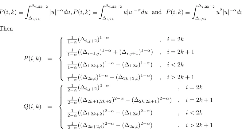
To evaluate the integral (23) when φj(y) is as in (11), define
P(i, k)≡
Z ∆i,2k+2
∆i,2k
|u|−αdu, P(i, k)≡
Z ∆i,2k+2
∆i,2k
u|u|−αdu and P(i, k)≡
Z ∆i,2k+2
∆i,2k
u2|u|−αdu.
Then
P(i, k) = 1
1−α(∆i,j+2)
1−α , i= 2k
1
1−α((∆i−1,j)
1−α+ (∆
i,j+1)1−α) , i= 2k+ 1 1
1−α((∆i,2k+2)
1−α−(∆
i,2k)1−α) , i <2k
1
1−α((∆2k,i)
1−α−(∆
2k+2,i)1−α) , i >2k+ 1
Q(i, k) = 1
2−α(∆i,j+2)
2−α , i= 2k
1
2−α((∆2k+1,2k+2)
2−α−(∆
2k,2k+1)2−α) , i= 2k+ 1 1
2−α((∆i,2k+2)
2−α−(∆
i,2k)2−α) , i <2k
1
2−α((∆2k+2,i)
2−α−(∆
and
R(i, k) =
1
3−α(∆i,i+2)
3−α , i= 2k
1
3−α((∆2k,2k+1)
3−α+ (∆
2k+1,2k+2)3−α) , i= 2k+ 1 1
3−α((∆i,2k+2)
3−α−(∆
i,2k)3−α) , i <2k
1
3−α((∆2k,i)
3−α−(∆
2k+2,i)3−α) , i >2k+ 1
Hence, using integration by substitution withh= (y−xi)/uin (23), we get
w0(xi) =
1 ∆1,0∆2,0
(R(i,0) + (∆1,i+ ∆2,i)Q(i,0) + ∆1,i∆2,iP(i,0)),
for i= 0,1, . . . , n
w2j(xi) =
R(i, j−1) + (∆2j−2,i+ ∆2j−1,i)Q(i, j−1) + ∆2j−2,i∆2j−1,iP(i, j−1)
∆2j−2,2j∆2j−1,2j
+R(i, j) + (∆2j+1,i+ ∆2j+2,i)Q(i, j) + ∆2j+1,i∆2j+2,iP(i, j) ∆2j+1,2j∆2j+2,2j
,
for j = 0,1, . . . ,n
2−1 and i= 0,1, . . . , n
wn(xi) =
R(i,n2 −1) + (∆n−2,i+ ∆n−1,i)Q(i,n2−1) + ∆n−2,i∆n−1,iP(i,n2 −1)
∆n−2,n∆n−1,n
,
for i= 0,1, . . . , n
and
w2j+1(xi) =
R(i, j) + (∆2j,i+ ∆2j+2,i)Q(i, j) + ∆2j,i∆2j+2,iP(i, j)
∆2j,2j+1∆2j+2,2j+1
,
for j = 0,1, . . . ,n
2−1 and i= 0,1, . . . , n
Appendix B
To evaluate the integral (24) when φj(y) as in (10), define
P(i, k)≡
Z ∆i,2k+2
∆i,2k
ln|u|du, Q(i, k)≡
Z ∆i,2k+2
∆i,2k
uln|u|du and R(i, k)≡
Z ∆i,2k+2
∆i,2k
Then
P(i, k) =
∆i,i+2ln ∆i,i+2−∆i,i+2 , i= 2k
∆2k,2k+1ln ∆2k,2k+1−∆2k,2k+1
+∆2k+1,2k+2ln ∆2k+1,2k+2−∆2k+1,2k+2 , i= 2k+ 1
∆i,2k+2ln ∆i,2k+2−∆i,2k+2−∆i,2kln ∆i,2k+ ∆i,2k , i <2k
∆2k,iln ∆2k,i−∆2k,i−∆2k+2,iln ∆2k+2,i+ ∆2k+2,i , i >2k+ 1
Q(i, k) = 1
2(∆i,i+2) 2ln ∆
i,j+2−14(∆i,i+2)2 , i= 2k 1
2(∆2k+1,2k+2) 2ln ∆
2k+1,2k+2−14(∆2k+1,2k+2)2
−12(∆2k,2k+1)2ln ∆2k,2k+1+14(∆2k,2k+1)2 , i= 2k+ 1 1
2(∆i,2k+2) 2ln ∆
i,2k+2−14(∆i,2k+2)2
−1 2(∆i,2k)
2ln ∆
i,2k+14(∆i,2k)2 , i <2k
1
2(∆2k+2,i) 2ln ∆
2k+2,i−14(∆2k+2,i)2
−12(∆2k,i)2ln ∆2k,i+14(∆2k,i)2 , i >2k+ 1
and
R(i, k) = 1
3(∆i,i+2) 3ln ∆
i,i+2−19(∆i,i+2)3 , i= 2k 1
3(∆2k,2k+1) 3ln ∆
2k,2k+1−19(∆2k,2k+1)3
+1
3(∆2k+1,2k+2)3ln ∆2k+1,2k+2−19(∆2k+1,2k+2)3 , i= 2k+ 1 1
3(∆i,2k+2) 3ln ∆
i,2k+2−19(∆i,2k+2)3
−13(∆i,2k)3ln ∆i,2k+19(∆i,2k)3 , i <2k
1 3(∆2k,i)
3ln ∆
2k,i−19(∆2k,i)3
Hence, using integration by substitution withh= (y−xi)/uin (24), we get
w0(xi) =
1 ∆1,0∆2,0
(R(i,0) + (∆1,i+ ∆2,i)Q(i,0) + ∆1,i∆2,iP(i,0)),
for i= 0,1, . . . , n
w2j(xi) =
R(i, j−1) + (∆2j−2,i+ ∆2j−1,i)Q(i, j−1) + ∆2j−2,i∆2j−1,iP(i, j−1)
∆2j−2,2j∆2j−1,2j
+R(i, j) + (∆2j+1,i+ ∆2j+2,i)Q(i, j) + ∆2j+1,i∆2j+2,iP(i, j) ∆2j+1,2j∆2j+2,2j
,
for j = 1, . . . ,n
2−1 and i= 0,1, . . . , n
wn(xi) =
R(i,n2 −1) + (∆n−2,i+ ∆n−1,i)Q(i,n2−1) + ∆n−2,i∆n−1,iP(i,n2 −1)
∆n−2,n∆n−1,n
,
for i= 0,1, . . . , n
and
w2j+1(xi) =
R(i, j) + (∆2j,i+ ∆2j+2,i)Q(i, j) + ∆2j,i∆2j+2,iP(i, j)
∆2j,2j+1∆2j+2,2j+1
,
for j = 0,1, . . . ,n
2−1 and i= 0,1, . . . , n
References
[1] Kendall E. Atkinson,The Numerical Solution of Fredholm Integral Equation of Second Kind, SIAM J. Numer. Anal. 4(1967) 337-348.
[2] Kendall E. Atkinson,A Survey of Numerical Methods for Solution of Fredholm Integral Equation of Second Kind, SIAM, Philadelphia, (1976).
[3] C.T.H. Baker, The Numerical Treatment of Integral Equation, Oxford University Press, (1977).
[4] Paola Baratella, A Note on the Convergence of Product Integration and Galerkin Method for Weakly Singular Integral Equations, J. Comp. App. Math. 85 (1997), 11-18.
[5] G.A. Chandler,Superconvergence of Numerical Solution of Second Kind Integral Equa-tion,Ph.D. Thesis, Australian National University, Canberra, (1979).
[6] Philip F. Davis & Philip Rabinowitz,Methods of Numerical Integration, 2nd edition, Academic Press,Inc, (1984).
[8] de Hoog & , R. Weiss,Asymptotic Expansions for Product Integration, Math. Comp. 27(1973), 295-306.
[9] G. Monegato & L. Scuderi,High Order Methods for Weakly Singular Integral Equa-tions with Non Smooth Input Function, Math. Comp. 67(1998), 1493-1515.
[10] Mohamad Rashidi Razali, Eigenvalue Problem in Integral Equations with Weakly Singular Kernels, Master Dissertation, University of Bath, School of Mathematics, (1975).