Bias in misspecified mixtures

r

Bias inMisspecifiedMixtures

Gerry Gray

Department of Statistics, North Carolina State University Box8203, Raleigh, North Carolina27695-8203,U.S.A.

SUMMARY

A finite mixture is a distribution where a given observation can come from any of a finite set of components. That is, the density of the random variable X is of the form f(x)

=

1I'₁f₁(x)

+

1I'2f2(x)

+ ... +

lI'kfk(x) , where the lI'i are the mixing proportions and the f_i are the component densities. Mixture models are common in many areas of biology; the most commonly applied is a mixture of normal densities. Many of the problems with inference in the mixture setting are well known. Not so well documented, however, are the extreme biases that can occur in the maximum likelihood estimators (MLEs) when there is model misspecification. This paper shows that even the seemingly innocuous assumption of equal variances for the components of the mixture can lead to surprisingly large asymptotic biases in the MLEs of the parameters. Assuming normality when the underlying distributions are skewed can also lead to strong biases. We explicitly calculate the asymptotic biases when maximum likelihood iscarried out assuming normality for several types of true underlying distributions. If the true distribution is -~ mixture of skewed components, then an application of the Box-Cox power transformation can reduce the asymptotic bias substantially. The power A in the Box-Cox transformation is in this case treated as an additional parameter to be estimated. In many cases the bias can be reduced to acceptable levels, thus leading to meaningful inference. A modest Monte Carlo study gives an indication of the small sample performance of inference procedures (including the power and level of likelihood ratio tests) based on a likelihood which incorporates estimation ofA. A real data example illustrates the method.

Institute of Statistics Mimeograph Series2227

July1992

Key Words: Normal mixtures; EM algorithm; Box-Cox transformation;

1. INTRODUCTION

A cancer treatment drug seems to cause a much more favorable response in some people than in others at the same dose level. A phenotypic characteristic in a species of pine tree is thought to be controlled by a gene with relatively few alleles. A length-frequency histogram of a sample of fIsh shows distinct modes corresponding to the ages 0, I, and 2 years. In each of these examples, the conceptual scientifIc model leads one naturally to the idea of a fInite mixture distribution, a distribution where a given observation can come from any of a fInite number of component distributions. Titterington, Smith, and Makov (1985) devote an introductory chapter to cataloging many such examples from such diverse fIelds as medicine, economics, geology, botany, and zoology.

Asa more specifIc example, we consider an experiment conducted to determine the feasibility of administering an oral vaccination to wild swine (Sus serafs). Wild swine may serve as reservoirs for diseases such as pseudorabies and swine brucellosis which can be transmitted to domestic swine. Thus it would be advantageous if wild swine could be easily innoculated against such diseases. A small experiment to determine the feasability of oral vaccination was conducted on Ossabaw Island, Georgia, by the Southeastern Cooperative Wildlife Disease Study, the Georgia Department of Natural

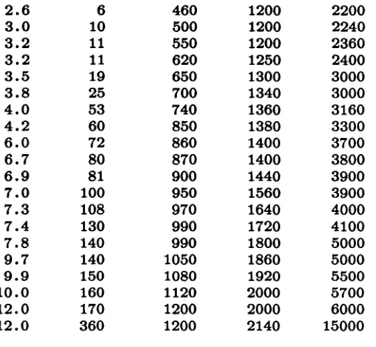
Resources, and the Ossabaw Foundation (Fletcher et al., 1990). Inthe fIrst stage of the study, twenty wild swine were captured and blood samples were drawn.· Then a grid of fIsh meal baits laced with iophenoxic acid was laid down. Iophenoxic acid is an organic iodine compound used as a diagnostic radiographic contrast agent in medical studies. After 2 days, and for 11 subsequent days, wild swine were captured and blood samples were drawn. Samples were collected from a total of 100 animals, 20 captured before the bait was distributed, 79 from captures after the baits had been presented, and one which ate a single bait while in captivity. The samples were analyzed for iophenoxic acid. The data (serum concentrations of iophenoxic acid from the 100 animals) are presented in Table 1 and in the histogram in Figure 1.

- Insert Table I, Figure 1

interest to determine whether the proportions of the mixture follow certain patterns, such as would be

produced if the population were in Hardy-Weinburg equilibrium.

The standard approach to estimation or hypothesis testing in the finite mixture setting is to use likelihood theory methods, assuming (possibly after a transformation) that the component distributions are normal. Often, to simplify computations, it is further assumed that the component distributions have the same variance. Typically, little attention is given to checking the validity of these assumptions. There isalsolittle information in the literature on the robustness of likelihood based inference procedures under misspecification of the component densities. Itis important, therefore, to point out that under certain types of misspecification there can beserious biases in the parameter estimates obtained. This includes misspecification of the parametric form of the mixture components as well as mistakenly assuming hom08kedasticity of the component densities. With these biases, tests about the proportions or about the parameters of the component distributions could go seriously astray.

This paper will identify, and hopefully resolve, some of the problems that can beencountered when there is misspecification in a finite mixture model. The remainder of Section 1 will cover notation and estimation techniques. Section 2 contains calculations of the asymptotic biases that arise under certain types of misspecification. Section 3 describes a bias-correction scheme utilizing the Box-Cox power transformation; Section 4 reexamines the asymptotic calculations of Section 2 after applying the power transformation. Section 5 presents the results of a small Monte Carlo experiment

investigating the small sample properties of the estimators and tests when the Box-Cox power transformation is included in the likelihood as a parameter tobe estimated. Finally, Section 6 will examine the swine innoculation data in more detail.

1.1 NOTATION

In a finite mixture, the density of the random variable X is of the form

where Pj

>

0, j =1· .. k ,and

E

j Pj = 1. The parameters Pj are called the mixing proportions and the functions f_{1 .} . • f_k are called the component densities of the mixture. Usually the f_j will have some specified parametric form and will bewritten f_j(x;9), where 9 is a vector of parameters. For example 9 wouldbea vector of locations and scales in a mixture of location-scale distributions. In most applications the f_j(x;9) are in fact assumed to benormal densities, so that we have

(1.1)

This paper will focus on the effect of departures from the normality assumption on the resulting parameter estimates and likelihood-based inference procedures.

There are three main problems that are encountered when developing inference procedures for mixture distributions. The first is the problem of determining the number of components. This issue will not be addressed in this paper. I assume throughout that the number of component distributions is known. See Ghosh and Sen (1985), Hartigan (1985), or McLachlan and Basford (1988) for further discussion. The second problem is related to estimation. There are both theoretical and practical difficulties to estimation in mixture distributions. Theoretically, difficulties arise with multiple local maxima of the likelihood surface and with identifiability of the mixture. Practically, convergence of the numerical procedures used to obtain estimates may be an issue. The computational procedures for obtaining maximum likelihood estimates (MLEs) for mixtures are usually fairly lengthy iterative processes which may not converge to an acceptable solution. However these computational difficulties seem to have been resolved somewhat with the advent ofthe EM algorithm (Redner and Walker, 1984). A third problem is that of misspecification of the component density type and of the variance structure (i.e., equal variances or not). This third problem has received little attention in the past, perhaps due to the overwhelming difficulty of the first two, but needs to be addressed, and is the focus of this paper.

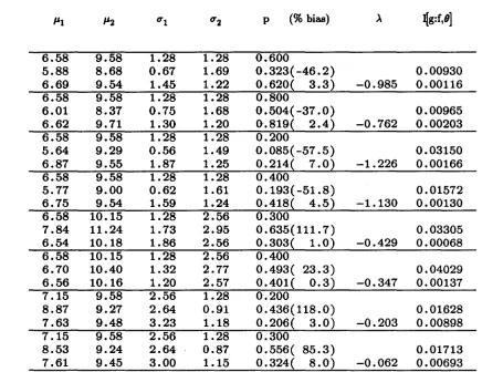
From the examples in the introduction it can be seen that many scientific models lead naturally to the idea of a finite mixture. However this does not mean that a mixture of normal distributions is the correct model to apply. To illustrate the consequences of incorrectly assuming normal component densities, Table 4 shows the estimates that would be obtained (as the sample size goes to infinity) when the true model is a mixture of extreme value distributions but the assumed model is a mixture of normal distribuitions. In the first case the mean of the first extreme value component is 6.58 but the estimated first component mean is 5.88. This corresponds to an asymptotic bias of 6.58 - 5.88

=

0.70 for estimating the mean of the first component. The bias in estimating the standard deviation of the first component is 1.28 - 0.67

=

0.61 and the bias in the mixing proportion p is 0.600 - 0.323

=

0.277. Many other entries in this table, and in Tables 3, 5, and 6, show comparable or greater asymptotic bias. Biases of such magnitude have serious implications for any type of inference based on the normal mixture model. Since skewness or nonnormality is often evident in biological data arising from a single-component population, such biases should be of great concern in biological applications of finite mixtures.

1.2 ESTIMATION TECHNIQUES

Historically many techniques have been usedto estimate the parameters of a mixture. Sinceclosed

form solutionsto the likelihood equations usually do not exist, the first efforts werebased either on the method of moments (e.g., Pearson, 1894; 1914)or were graphical in nature (e.g., Fowlkes, 1979).

Today with fast computers and the EM algorithm of Dempster, Laird, and Rubin (1977), maximum likelihood seems to be the method of choice. See McLachlan and Basford (1988,section 1.2)for a brief history.

The general ideato the EM algorithm is to cast the problem in a missing data framework, thus making solutions to the likelihood equations more tractable. That is, think of the full data as

(Xi,Zil,Zi2'· .. ,zik) where the Zij are indicator variables for membership in thejthcomponent. For example, an observation from the second component of the mixture would have si

=

(0,1,0,0, ... 0).

Ifthe Zij were known, then the maximum likelihood estimators for the parameters would simply be the MLEs from each of the component groups. However, the data we actually observe has the Zij missing. The EM algorithm consists of the following two steps repeated alternatively until some criterion for convergence is met.

M step: find ,(

m+

1) to maximize the full data likelihood conditional on the wij

The likelihood is guaranteed to be nondecreasing at each iteration of the EM algorithm (Dempster et al., 1977; Wu, 1983),but the algorithm can be slow to converge. More details on implementation of EM in the mixture model can be found in Titterington et al. (1985, Ch. 4) or in Redner and Walker

(1984).

2. BIASES ARISING FROM MISSPECIFICATION

Ifthe true underlying density is specified correctly, then maximum likelihood via the EM algorithm should give parameter estimates which are asymptotically unbiased. However, if in fact the underlying mixture is not specified correctly, then the ML estimators can have substantial asymptotic biases. In order to investigate these biases I numerically calculate the probability limit of the MLEs assuming

normal component densities for a range of true underlying distributions. That is, I calculate the estimates that would be obtained, when normality is assumed, as the sample size increases to infinity. I also calculate the "distance" between the true density and the density obtained by substituting the limiting values of the MLE for' in (1.1). This "distance" measure is the Kullback-Leibler distance (or Kullback-Leibler information criterion, KLIC) I[g:f,lJI

=

flog [g(x)] g(x) dx - flog [f(Xi')] g(x) dx, where g(x) is the true underlying density and f(Xi') is the assumed parametric form. SeeWhite(1982), Hernandez and Johnson (1980), Kullback and Leibler (1951), or Titterington et al. (1985, p. 114-117) for some discussion of the use of this distance measure.

From Jennrich (1969, theorem 2), we know that under suitable regularity conditions

sup

ft

1:

log f(Xi')

~

sup

'eC

'eC

00

J

log f(Xi') g(x) dx

-00

where f(Xi') is the assumed density, g(x) is the true density, and C is a compact subset of the parameter space. It then follows that the MLE

iJ

is strongly consistent for the parameter vector (J* which maximizes the above limiting integral (e.g., White 1982, theorem 2.2) Thus by calculation of

(J* which maximizes flog [f(Xi(J)] g(x) dx for a specified g(x), we obtain the value of the limiting MLE for (Jwhen f(xj(J) is the assumed parametric form and g(x) is the true density. Further calculation of

J

log [g(x)] g(x) dx leads to the minimum KLIC distance between g(x) and f(xj(J), l[g:f,9*].

I calculate an approximation to the limiting integration/maximization by an application of the midpoint rule and the EM algorithm. As a check on the accuracy of the numerical integration I include in the calculations a correctly specified model where the estimates should be asymptotically unbiased and the KLIC should be

o.

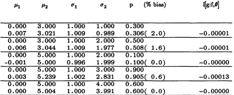
Results for 5 different cases are given in Table 2. The calculated probability limits were within 2% of their true value and the KLIC was less than .00013 for each of these integrations. This gives some indication of the numerical accuracy of the

maximization/integration scheme used.

Insert Table 2 here

-The types of misspecification investigated were:

1. Actual parametric family is a mixture of two normals with unequal variances, but the model used specified equal variances (10 different cases)

-4. Actual parametric family is a mixture of two Laplace distributions (6 different cases)

The first case was fit with a mixture of two normals with equal variances. Often in practice mixture models are fit with equal variances eitherto get around some problems of convergence and/or local maxima or toachieve parsimony and presumably greater precision of estimation.

The last three types of misspecification represent skewed or heavy tailed distributions. The assumed model for these three cases was a mixture of two normals with unequal variances ( eq. 1.1). Figure 2 illustrates one particular case, correspondingtothe first three rows in Table 4. The solid line is the true g(x), in this example a mixture of two extreme value distributions with location parameters 6 and 9, scale parameters 1 and 1, and mixing proportion 0.6. Note that in order to make meaningful comparisons with a mixture of two normal distributions the entries in Tables 4-6 are in terms of means and standard deviations, e.g., an extreme value distribution with location 6 and scale 1 has mean 6.58 and standard deviation 1.28. The dotted line in Figure 2 indicates the fit that would be obtained asymptotically when the assumed model is a mixture of two normals. In a sense this is the normal mixture that is "closest" to this particular g(x). Here 1[g:f,tJ] is .0093. The dashed line indicates the fit that would be obtained when an additional parameter for skewness is included in the model (see Section 3). Adding a skewness parameter reduces l[g:f,tJ] to .0012 and reduces the asymptotic bias in the MLE for p from 46% to 3%.

- Insert Figure 2, Tables 36 here

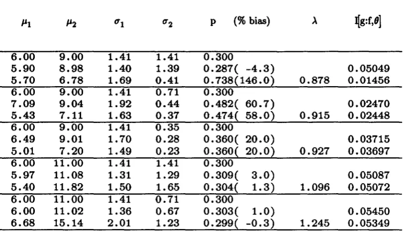
-The results of the bias calculations are given in Tables 3 - 6. For each of the misspecifications considered, there were substantial biases. Under the mixture distributions considered, the probability limits of the ML estimators were often substantially different than the true parameter values. In addition, the KLIC was in general much larger before a skewness parameter was included in the model. In the context of 2 component mixtures, our calculations suggest that a "good fit" will have a KLIC of about .002 or less. Values of the KLIC ranging from .01 to .12 indicate a large deviation from the true distribution. Hernandez and Johnson (1980) gave some values of the KLIC in the context of

transformations to normality for single component distributions. The relative lack of flexibility in the single component distributions leads to a much greater range in KLIC values than are obtained with 2 component mixtures. That is, for a single component distribution a good fit will have a KLIC of less than .01 while a poor fit will have a KLIC ranging from about .01 to 1.0. Note that our I [g:f,tJ] is equivalent to I[g:<p_JJzuz] in Hernandez and Johnson (1980).

The implications of these calculations are that misspecification of the model can lead to large biases in parameter estimates. In practice, this means that inference carried out without taking into

account the possibility of model misspecification may go seriously astray. If there is misspecification, confidence intervals for the parametersbased on the inverse of the observed information matrix j-l can

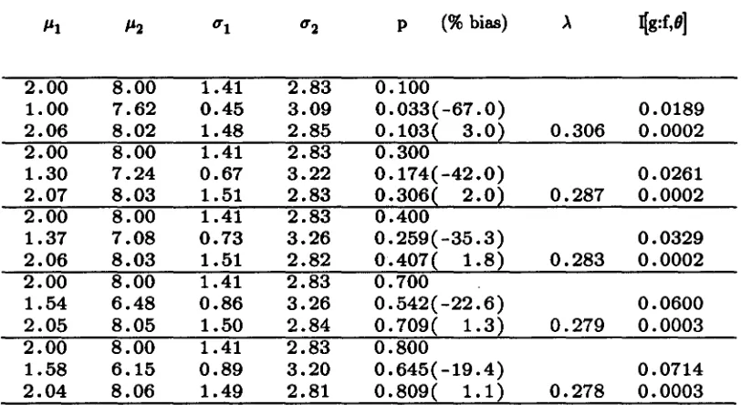
beincorrect for two reasons: the estimators themselves are biased and j-l calculated assuming normality is incorrect. Tables4and5show clearly that if the underlying density is a mixture of skewed distributions, then fitting a mixture of normal distributions will give biased results no matter how large the sample. Table 3 shows that even with normality, estimation under the false assumption of equal variances can leadto a large bias in estimates of the means Pi and the mixing proportion p.

3. TRANSFORMATION TO A NORMAL MIXTURE

One possible solution to the bias problem is to attempt to correct the miBBpecification by transforming the data to a mixture of normal distributions. A common approach in the single component caseisto apply the Box-Cox family of power transformations to the data and then perform the estimation and testing aBBuming normality. For x

>

0, the Box-Cox transformationisgiven by (Box and Cox, 1964):

={

X"\-1

(..\) -..\- ..\~O x - log(x) ..\=0.

Ifwe aBBume that the true mixture distribution can in fact betransformed to a mixture of normals 1

with the above transformation (only the casewhen x = (1+..\v)X or x=evj va normal r.v.), then we

can write the full data log likelihood as:

(3.1)

Now we can find the MLEs for the parameters(Jand ..\ using BOme form of numerical maximization. I

used Newton's method in the M step of the EM algorithm to maximize this likelihood. Thus to apply the EM algorithm, the E step proceeds essentially as in the simpler casecorresponding to (1.1), while the M stepis now a numerical maximization of the likelihood (3.1) conditional on the Wij.

Note that for a fixed ..\ the likelihood in (3.1) is just

E

(..\-1) In(xi) plus the normal likelihood from (1.1), based on the transformed data

x~..\).

Thus an alternative maximization scheme would be to compute the

x~..\)

for a grid of possible..\ values, apply the EM algorithm to find the MLEs for the remaining parameters, and adjust the likelihood by adding

E

(..\-1) In(xi). This scheme has three main advantages. First, for a given ..\, it is much simpler computationally as no numerical

examined and the possibility of missing a maximum if the" grid is not fine enough.

Hernandez and Johnson (1980) discuss the application of the Box-Cox transformation to a single component density, and give some indications of how closely the transformed density can approximate the normal, where "closeness" is measured using the Kullback-Leibler distance measure. They show that the Box-Cox transformation can (at least asymptotically) transform a fairly wide variety of skewed densities ( e.g., gamma, Weibull, inverse gaussian) to a close approximation to the normal. The extreme value density can also be brought quite close tothe normal with such a transformation, using"

=

.872 - .288(J/

e,

where(Jand

e

are the extreme value location and scale parameters. So even when exact normality cannot be achieved by application of a power

transformation, in many cases the distribution ofXC")may be closely approximated by a normal distribution. The Box-Cox transformation seems to work well on skewed distributions as long as f(x)

=

0at the boundaries of support, but not on heavy or light tailed symmetric distributions.

Note that the Kullback-Leibler distance measure is the same whether calculated on the original or transformed scale. That is, we can either measure the distance between the true distribution and the back-transformed mixture of normals or we can measure the distance between the Box-Cox

transformed true distribution and the mixture of normals.

Also note that in the usual application of the Box-Cox transformation it is assumed that we "measured on the wrong scale" and are now merely transforming to the correct scale. The common application of the log ("=0) or the square root ("=!) transformations are examples. For a mixture distribution, assuming a common value of " for each of the component densities seems consistent with this view of the Box-Cox transformation. But we could also think of the transformation power " as just another parameter that is a measure of skewness, and assume a different

"i

for each component of the mixture. However, numerical calculations showed that for the cases in Tables 4-6, assuming different \ gave only a marginal improvement in the fit. As numerical problems associated with estimation are increased by fitting different

"i'

it seemed best for philosophical and practical reasons to investigate a procedure which assumed a single skewness parameter, i.e., the same" for all

components of the mixture.

MacLean et al. (1976) propose a similar procedure for using a transformation to resolve problems with skewness in "commingled" distributions. Unfortunately they provide no information concerning the properties of their procedure. For example, they propose centering and scaling the data before estimating, which makes the transformation parameter" difficult to interpret. Further, they do not provide any explicit calculations as to the biases that occur under misspecification, and they carry out their estimation assuming equal variances for each of the components.

4. BIASES REVISITED

To evaluate the effectiveness of the transformation scheme, I compare the asymptotic biases of the MLEs based on the likelihood (3.1) with the biases obtained under (1.1). The probability limits of parameter estimates assuming (1.1) and (3.1) are giveninthe second and third of each set of three lines in Tables 4 - 6. The transformation seems to work quite well in reducing the asymptotic bias of the estimators for skewed distributions. As expected, biases for the heavy-tailed but symmetric Laplace distribution were not reduced. But the considerable reduction in bias for the skewed

distributions suggests that likelihood theory inference procedures based on (3.1) as the "correct" model may be a reasonable approach in practice.

5. MONTE CARLO RESULTS

Ifstrong biases exist in the MLEs under model misspecification, then inferences based on maximum likelihood could go seriously astray. If the proposed transformation can substantially reduce the bias problems, it should also lead to more reliable inference.

A small Monte Carlo study was undertaken to assess the finite sample properties of the

proposed estimation scheme. In addition to examining bias of point estimates, I wished to evaluate the effect of including a power transformation on the performance of specific likelihood ratio tests. Small sample biases in the parameter estimates are also of concern since the bias calculations done previously were asymptotic, indicating what would be attained with very large samples. Ifthe power

transformation cannot substantially reduce biases with samples of say, 200, then another approach needs to be considered.

The Monte Carlo samples consisted of data generated from two component mixtures, where the components were either normal, extreme value, or lognormal distributions. For discussion purposes, denote a sample of size 200 from a mixture of two normals with means 8 and 13, standard deviations 1 and 2, and mixing proportion .3 for the first component as (N 8 13 1 2 .3 200). Similarly denote a sample from a mixture of two extreme value distributions with location parameters 8 and 13, scale parameters 1 and 2, and mixing proportion .3 as (EV 8 13 1 2 .3 200). Various combinations of means, variances, and sample sizes for the two components were chosen to give some insight into the properties of the estimators and likelihood ratio tests. For each situation, 100 Monte Carlo samples were

generated.

For each data set generated, ten different models were fit and estimates were saved along with the associated likelihoods. Thus a number of interesting likelihood ratio tests could be calculated for

each fit. The emphasis was on likelihood ratio tests for the three null hypotheses Ho: ~= 1, H_O:ul=u2' and Ho: P=Po ( Po a specified proportion). The tests concerning the u's and the p's could beconducted with and without including~in the model, i.e., either estimating ~or assuming ~= 1. In addition, If

considered a tw~stage test which consisted of first testing Ho:~=1(at a significance level a= .20) and then proceeding to test Ho:u1=0'2or Ho:p=po using ~in the model only if the first test rejected. Such a test should protect against misspecification and at the same time provide a simpler model where appropriate. Finally, to assess the power of the likelihood ratio test for hypotheses about p, I fit models with p constrained to various values and calculated likelihood ratio tests.

Thus for each Monte Carlo sample generated, seven likelihood ratio tests were carried out:

Ho:~=1 in (3.1); _Ho:u1=u2assuming normality; Ho:p=Po assuming normality; _HO:u1=u2with the Box-Cox parameter ~estimatedj Ho:p=po with ~estimatedj and the two stage tests for Ho:u1=0'2 and Ho:p=po. Note that critical values for the test statistics were basedon a X2distribution of

-210g~ji.e., basedon standard likelihood theory.

The mean values of the parameter estimates from the Monte Carlo study were very similar to the asymptotic values calculated as described in section 2. Thus it appears as if the small sample biases are essentially the same as the asymptotic biases, at least for sample sizes and mixtures considered here.

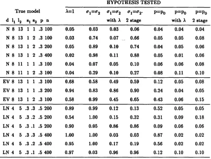
Table 7summarizes the results of these likelihood ratio tests. Note that for a binomial r.v. with p = .05 the standard error of

f>

from a sample of size 100 is approximately .022. Thus an approximate 95%d. for an entry in the table would be

±

.044.

- Insert Table7here

-First consider the tests for ~= 1. In general, the results here were quite favorable. Under the normal mixtures, the LRT held its level, with 2 to 5 percent rejection of the null for a test with

nominal size .05. In addition, the power of the test under the extreme value and lognormal models was good, ranging from 58 to 100 percent rejections. So inferences about ~ based on the LRT appear to be valid, and to have fairly good power when the true underlying distributions are mixtures of lognormals or extreme values. From this we might infer that LRT based inferences about ~will beat least approximately valid for mixtures of skewed distributions in general, at least when the component distributions are reasonably far apart and p is not too near 0 or 1.

For the normal mixture, all three tests for 0'1= 0'2 (i.e., the test assuming normality, or~ = Ij the test with ~ estimated; and the two stage test) held their level well. The test with ~ estimated had low power, but the two stage procedure had power comparable to that of the test where ~was assumed

to equal 1. Itappears that thereisa certain amount of non-identifiability between ~and the twotT

parameters in the sense that a power transformation affects the scale of the components of the mixture differently, and can thus adjust somewhat for differenttT parameters.

In the extreme value mixtures the tests oftTl

=

_tT2 are not informative. The "correct" tests (i.e., with ~estimated) had reasonable power. Note that the test oftTl

=

tT₂istesting whether the two

tT parameters are the same after the transformation isapplied, not before. Thus we would hope that

these tests would reject a large percentage of the time. Also note that strictly speaking, even with ~

included, the model (3.1) still does not specify the true underlying distribution correctly. No power transformation can bring an extreme value distribution to exact normality; the Box-Cox~is the power that brings the mixture "closest" as measured by the Kullback-Leibler distance.

The lognormal mixtures are more interesting, since in this case thereisa transformation that will bring the mixture to exact normality, i.e., ~= 0 or a log transform. Note that the tests under misspecification (i.e., ~

=

1 assumed) were very unreliable. For example, the case (LN 4 5 .3 .3 .5400) rejected the hypothesis that tTl

=

tT2 in 100 out of 100 Monte Carlo samples under misspecification,

while the correct test (i.e., ~estimated) rejected in only 3 samples, for a test with nominal size .05. In this case a log transformation would result in a normal mixture with equal variances (N 4 5 .3 .3 .5 400), so this test should reject 5% of the time. Results for this mixture with a Monte Carlo sample size of 200 showed a similar pattern, although in this case the test with ~estimated was somewhat liberal, rejecting in 12 out of 100 samples. The two stage test seemed to perform well here also, mostly yielding results (in terms of numbers of rejections) similar to those for the test with ~ estimated.

The tests for p

=

Poseemed to be valid in the normal mixtures investigated. For the mixtures of skewed distributions, the tests under model misspecification were extremely liberal. There were from 9 to 87 rejections (nominal size .05) out of 100 Monte Carlo samples. In contrast, the test with ~

estimated held its level well, and the two stage test appeared liberal in only two out of the nine cases considered.

To investigate the power of the tests for p, additional fits and likelihood ratio tests were calculated for p=.25, p= .50, or p= .60, depending on the underlying model. Table 8 summarizes these results. The p's chosen in each case bracketed the true p (Le., one above and one below). In general these tests performed as expected, with higher power with larger samples or with increasing difference between the hypothesized and the true value of p. One initially surprising result was the seeming loss of power for the lognormal cases when the fitted model included estimation of~.

'.

- Insert Table 8 here

-To summarize, it appears that the concerns about tests under misspecification raised by the

asymptotic bias calculations were realizedinsmall samples. Ifthe model is erroneously specified as a mixture of normals when in fact the data arise from a mixture of skewed distributions, then serious problems arise in likelihood ratio tests. Application of the Box-Cox transformation during the

estimation process seems to make the tests more valid, although at the expense of a loss of power when testing(T1

=

(T2' A two-stage procedure, akin to the common practical procedure of basing inferences

on a reduced model after a preliminary test against a larger model, seems to improve the power somewhat with little effect on the level of the tests.

6. EXAMPLE

As an example, we now look more closely at the swine innoculation experiment from the Introduction. In this particular example, additional information about the mean and variance of one of the

components is provided by the 21 fully classified observations (i.e., the 20 swine who were known not to have eaten any baits and the 1 who ate 1 bait). However, these classified observations do not provide any information about the proportions in each group since they were not sampled randomly with regard to their group membership. These "fully classified" observations make the likelihood of 2.1 slightly more complex, but do not change the overall procedure used. See McLachlan and Basford (1987; pp. 29-31,40) for details of the likelihood calculations when some of the data are fully classified.

The swine come upon the bait sites while foraging. When they encounter a site where baits are laid out, they can eat none, one, or more baits. Since each bait contains 2 ml of 10 mg IA/ml corn oil, a reasonable model of the distribution of iophenoxic acid in the blood samples might be a mixture distribution with components corresponding to dose levels of 0, 20, and 40 or more milligrams iophenoxic acid. A three component mixture fit to the swine dataispresented in Figure 3.

- Insert Figure 3

-Maximum likelihood estimates of the means of the three components after transformation were 1.84, 4.18, and 6.21. MLEs for the standard deviations were 0.52,0.30, and 0.48. Standard error estimates were calculated by numerically differentiating the likelihood surface, and are shown in Figure

3.

The MLE ~was -0.048, quite close to a log transformation. A grid search over A revealed a local maximum of the likelihood at ~= _{.127. A LRT of Ho:}A=O was not significant, thus a log transformation of the data would be reasonable. 95% confidence bounds for A based on a likelihood

profile were (-0.38, 0.52), bounds based on ~and the numeric estimate of I-I were (-0.38, 0.29). A likelihood ratio test of Ho: ~

=

1 for a three component mixture gave a X2statistic of 36.113

(1 df, p

<

.0001), strongly rejecting normality of the components for this example.

Estimates of the proportions of the swine who ate 0,1, and 2 or more baits were .076, .164, and .760, respectively. Thus it appears that over 92% of the swine ate at least one of the baits, and 76% ate two or more baits. Fitting a 3 component mixture to the untransformed data gave

proportions of .048, .700, and .252. There is a marked difference in the estimates of the second and third proportions between the transformed and untransformed fit. The first proportion is not affected quite as much, probably partly due to its small size and partly due to the large number of fully classified observations known to have come from this component.

The experimenters themselvesuseda simpler approach to the analysis. Based on the 20 wild swine captured before baiting, they calculated a cut-off of 3 sample standard deviations above the mean and separated the 79 remaining unclassified animals into two groups based on this value. No transformation of the data was attempted. Thus 76 animals with iophenoxic acid levels greater than 15.62 mg/IOO ml were classified as having eaten at least one bait, giving a 95% success rate. So the experiment was declared a "success" in that it could be a cost effective method for delivery of vaccine to wild swine (Fletcher et al. ,1990).

7. CONCLUSIONS

Many scientific models lead naturally to a finite mixture model. The usual assumption is that of a normal mixture, but asymptotic calculations show that likelihood-based inferences under such a model are not robust to misspecification. In particular, if the true model is a mixture of skewed distributions, then large biases can result in the parameter estimates, and inferences based on likelihood theory and the normal mixture model can go seriously astray. However, the incorporation of a Box-Cox type power transformation into the model can reduce the bias substantially if the underlying distributions are skewed. A Monte Carlo study investigating the properties of likelihood ratio tests using such a transformation gave encouraging results.

ACKNOWLEDGEMENTS

Data for the example were used with permission of the Southeastern Cooperative Wildlife Disease Study.

..

REFERENCES

Box, G.E.P., and Cox, D.R. (1964). An analysis of transformations. Journalofthe Royal Statistical Society, Series B26, 211-252.

Dempster, A.P., Laird, N.M., and Rubin, D.B. (1977). Maximum likelihood from incomplete data via the EM algorithm. Journalofthe Royal Statistical Society, Series B39, 1-22. Fletcher, W.O., Creekmore, T.E., Smith, M.S., and Nettles, V.F. (1990). A field trial to

determine the feasability of delivering oral vaccines to wild swine. JournalofWildlife Diseases26, 502-510.

Fowlkes, E.B. (1979). Some methods for studying the mixture of two normal (lognormal) distributions. Journalofthe American Statistical Association74, 561-575.

Ghosh, J.K., and Sen, P.K. (1985). On the asymptotic performance of the log likelihood ratio statistic for the mixture model and related results. In Proceedingsofthe Berkeley

Conference in HonorofJerzy Neymanand Jack Keifer, Volume II, L.M. Le Cam and R.A. Olshen (eds). Wadsworth.

Hartigan, J.A. (1985). A failure of likelihood asymptotics for normal mixtures. In Proceedings ofthe Berkeley Conference in HonorofJerzyNeymanand Jack Keifer, Volume II,

L.M. Le Cam and R.A. O1shen (eds). Wadsworth.

Hernandez, F., and Johnson, R.A. (1980). The large-sample behavior of transformations to normality. Journalofthe American Statistical Association 75, 855-861.

Jennrich, R.I. (1969). Asymptotic properties of non-linear least squares estimators. AnnalsofMathematical Statistics40, 633-643.

Kullback, S., and Leibler, R.A. (1951). On information and sufficiency. AnnalsofMathematical Statistics 22, 79-86.

MacLean, C.J., Morton, N.E., Elston, R.C., and Yee, S. (1976). Skewness in commingled distributions. Biometrics36, 695-699.

McLachlan, G.J., and Basford, K.E. (1987). Mixture models: Inference and Applications to Clustering. New York: Marcel Dekker.

Pearson, K. (1894). Contribution to the mathematical theory of evolution. Philosophical Transactionsofthe Royal Society, SeriesA 185, 71-110.

Pearson, K. (1914). A study of Trypanosome strains. Biometrika10, 85-143.

Redner, R.A., and Walker, H.F. (1984). Mixture densities, maximum likelihood and the EM algorithm. Society for Industrial and Applied Mathematics Review26, 195-239.

White, B. (1982). Maximum likelihood estimation of misspecified models.

Econonmetrica50, 1-25.

Wu, C.J. (1983). On the convergence properties of the EM algorithm.

The Annals of Statistics11, 95-103.

..

Table 1

Data from the wild swine innoculation experiment. Values are pg iodine / 100 ml serum in samples drawn from captured wild swine. The first column are data from the swine captured before the baits

were set. The largest observation (15000) was excluded from the analysis as an outlier.

2.6 6 460 1200 2200

3.0 10 500 1200 2240

3.2 11 550 1200 2360

3.2 11 620 1250 2400

3.5 19 650 1300 3000

3.8 25 700 1340 3000

4.0 53 740 1360 3160

4.2 60 850 1380 3300

6.0 72 860 1400 3700

6.7 80 870 1400 3800

6.9 81 900 1440 3900

7.0 100 950 1560 3900

7.3 108 970 1640 4000

7.4 130 990 1720 4100

7.8 140 990 1800 5000

9.7 140 1050 1860 5000

9.9 150 1080 1920 5500

10.0 160 1120 2000 5700

12.0 170 1200 2000 6000

Table 2

Asymptotic bias calculations for five different mixtures of two normal distributions fit with different variances, i.e. a correctly specified model. The first of each pair of rows indicates the true means and standard deviations of the component distributions. The second row of each set shows the asymptotic limits of the maximum likelihood parameter estimates, calculated by numerical integration. This table

should give some indication of the accuracy of the numerical integrations used in the bias calculations. The percent bias in estimates of p are indicated in parentheses. ~g:f,9] is the asymptotic

Kullback-Leibler distance between the true mixture and the fitted model.

1'1 1'2 0'1 0'2 p (% bias) ~g:f,9]

0.000 3.000 1.000 1.000 0.300

0.007 3.021 1.009 0.989 0.306( 2.0) -0.00001

0.000 3.000 1.000 2.000 0.500

0.006 3.044 1.009 1.977 0.508( 1.6) -0.00001

0.000 5.000 1.000 2.000 0.100

-0.001 5.000 0.996 1.999 0.100( 0.0) -0.00000

0.000 5.000 1.000 3.000 0.900

0.003 5.239 1.002 2.831 0.905( 0.6) -0.00013

0.000 5.000 1.000 4.000 0.600

".

Table 3

Asymptotic bias calculations for 10 different mixtures of two normal distributions fit with equal variances. The first of each pair of rows indicates the true means and standard deviations of the component distributions. The second row of each pair shows the asymptotic limits of the maximum likelihood parameter estimates, calculated by numerical integration. The percent bias in estimates of p

are indicated in parentheses. ~g:f,,] is the asymptotic Kullback-Leibler distance between the true mixture and the fitted model.

PI P2 0'1 0'2 p (%bias) ~g:f,,]

0.000 3.000 1.000 2.000 0.300

0.760 4.211 1.469 1.469 0.612(104.0) 0.00806 0.000 3.000 1.000 2.000 0.500

0.432 4.297 1.326 1.326 0.724( 44.8) 0.01312 0.000 3.000 1.000 3.000 0.200

0.995 5.517 2.109 2.109 0.689(244.5) 0.02762 0.000 3.000 1.000 3.000 0.700

0.203 5.714 1.386 1.386 0.874( 24.9) 0.04110 0.000 5.000 1.000 2.000 0.100

1.300 5.334 1.810 1.810 0.207(107.0) 0.00708 0.000 5.000 1.000 2.000 0.400

0.485 5.560 1.535 1.535 0.504( 26.0) 0.03265 0.000 5.000 1.000 3.000 0.700

0.280 6.774 1.483 1.483 0.812( 16.0) 0.08323 0.000 5.000 1.000 3.000 0.900

0.077 6.763 1.174 1.174 0.937( 4.1) 0.05034

0.000 5.000 1.000 4.000 0.600

0.443 8.042 1.890 1.890 0.795( 32.5) 0.11588 0.000 5.000 1.000 4.000 0.800

Table 4

Asymptotic bias calculations for 8 different mixtures of two extreme value distributions. The first of each set of rows indicates the true means and standard deviations of the component distributions.

Note that 6.58 isthe mean of an extreme value distribution with location parameter 6 and scale parameter 1, 10.15is the mean of an extreme value distribution with parameters 9 and 2, etc. The second row of each set shows the approximate asymptotic limits of the maximum likelihood parameter

estimates, calculated by numerical integration. The third row of each set shows these limits calculated with an additional parameter for skewness included in the model. The percent bias in estimates of p

are indicated in parentheses. qg:f,'] isthe asymptotic Kullback-Leibler distance between the true mixture and the fitted model.

1'1 1'2 0'1 0'2 P (%bias) qg:f,O]

6.58

9.58

1.28

1.28

0.600

5.88

8.68

0.67

1.69

0.323(-46.2)

0.00930

6.69

9.54

1.45

1.22

0.620(

3.3)

-0.985

0.00116

6.58

9.58

1.28

1.28

0.800

6.01

8.37

0.75

1.68

0.504(-37.0)

0.00965

6.62

9.71

1.30

1.20

0-.

819(

2.4)

-0.762

0.00203

6.58

9.58

1.28

1.28

0.200

5.64

9.29

0.56

1.49

0.085(-57.5)

0.03150

6.87

9.55

1.87

1.25

0.214(

7.0)

-1.226

0.00166

6.58

9.58

1.28

1.28

0.400

5.77

9.00

0.62

1.61

0.193( -51.8)

0.01572

6.75

9.54

1.59

1.24

0.418(

4.5)

-1.130

0.00130

6.58

10.15

1.28

2.56

0.300

7.84

11.24

1.73

2.95

0.635(111. 7)

0.03305

6.54

10.18

1.86

2.56

0.303(

1.0)

-0.429

0.00068

6.58

10.15

1.28

2.56

0.400

6.70

10.40

1.32

2.77

0.493( 23.3)

0.04029

6.56

10.16

1.20

2.57

0.401(

0.3)

-0.347

0.00137

7.15

9.58

2.56

1.28

0.200

8.87

9.27

2.64

0.91

0.436(118.0)

0.01.628

7.63

9.48

3.23

1.18

0.206(

3.0)

-0.203

0.00898

7.15

9.58

2.56

1.28

0.300

8.53

9.24

2.64

0.87

0.556( 85.3)

0.01713

7.61

9.45

3.00

1.15

0.324(

8.0)

-0.062

0.00693

.-'.

Table 5.

Asymptotic bias calculations for five different mixtures of two gamma distributions. The first of each set of rows indicates the true means and standard deviations of the component distributions. The second row of each set shows the asymptotic limits of the maximum likelihood parameter estimates, calculated by numerical integration. The third row of each set shows these limits calculated with an

additional parameter for skewness includedinthe model. The percent bias in estimates of p are indicated in parentheses. ~g:f,6] is the asymptotic Kullback-Leibler distance between the true mixture

and the fitted model.

PI P2 0'1 0'2 p (%bias) ~g:f,6]

2.00

8.00

1.41

2.83

0.100

1.00

7.62

0.45

3.09

0.033(-67.0)

0.0189

2.06

8.02

1.48

2.85

0.103(

3.0)

0.306

0.0002

2.00

8.00

1.41

2.83

0.300

1.30

7.24

0.67

3.22

0.174(-42.0)

0.0261

2.07

8.03

1.51

2.83

0.306(

2.0)

0.287

0.0002

2.00

8.00

1.41

2.83

0.400

1.37

7.08

0.73

3.26

0.259(-35.3)

0.0329

2.06

8.03

1.51

2.82

0.407(

1.8)

0.283

0.0002

2.00

8.00

1.41

2.83

0.700

1.54

6.48

0.86

3.26

0.542(-22.6)

0.0600

2.05

8.05

1.50

2.84

0.709(

1.3)

0.279

0.0003

2.00

8.00

1.41

2.83

0.800

1.58

6.15

0.89

3.20

0.645(-19.4)

0.0714

Table 6

Asymptotic bias calculations for 5 different mixtures of two Laplace distributions. The first of each set of rows indicates the true means and standard deviations of the component distributions. Note that

1.41 is the standard deviation of a Laplace distribution with scale parameter 1. The second row of each set shows the asymptotic limits of the maximum likelihood parameter estimates, calculated by

numerical integration. The third row of each set shows these limits calculated with an additional parameter for skewness included in the model. The percent bias in estimates of p are indicated in parentheses. ~g:f,tI] is the asymptotic Kullback-Leibler distance between the true mixture and the

fitted model.

1'1 1'2 (11 (12 P (%bias) ~g:f,8]

6.00

9.00

1.41

1.41

0.300

5.90

8.98

1.40

1.39

0.287( -4.3)

0.05049

5.70

6.78

1.69

0.41

0.738(146.0)

0.878

0.01456

6.00

9.00

1.41

0.71

0.300

7.09

9.04

1.92

0.44

0.482( 60.7)

0.02470

5.43

7.11

1.63

0.37

0.474( 58.0)

0.915

0.02448

6.00

9.00

1.41

0.35

0.300

6.49

9.01

1.70

0.28

0.360( 20.0)

0.03715

5.01

7.20

1.49

0.23

0.360( 20.0)

0.927

0.03697

6.00

11.00

1.41

1.41

0.300

5.97

11.08

1.31

1.29

0.309(

3.0)

0.05087

5.40

11.82

1.50

1.65

0.304(

1.3)

1.096

0.05072

6.00

11.00

1.41

0.71

0.300

6.00

11.02

1.36

0.67

0.303(

1.0)

0.05450

Table 7

Percent rejections for likelihood ratio tests in Monte Carlo simulations. The true model is listed in the first columns, with the heading I'd 11 12 sl s2 p nIt indicating the distribution type, location parameters, scale parameters, mixing proportion, and sample size for the particular

..

mixture used. The notation EV 8 13 12.3 100, for example, indicates that the true distribution consisted of a mixture of two extreme value distributions with location parameters

8 and 13, scale parameters 1 and 2, mixing proportion .3 for the first component, and a sample size of 100 in each Monte Carlo sample. There were 100 Monte Carlo samples for each

model. The two stage test procedure consisted of first testing Ho:~=1at a=.20 and then

HO:0'1=0'2or Ho:p=po at a=.05 with ~estimated only ifthe first test rejected. Tests without ~

estimated for the extreme value and lognormal cases are misspecified.

HYPOTHESIS TESTED

True model ~=1 0'1=0'2 0'1=0'2 0'1=0'2· P=Po P=Po P=Po

d 11 12 s1s2 p n with ~ 2 stage with ~ 2 stage

N 8 13 1 1 .3 100 0.05 0.03 0.03 0.06 0.04 0.04 0.04

N 8 13 1 2 .3 100 0.03 0.74 0.07 0.66 0.05 0.05 0.08

N 8 13 1 2 .3200 0.05 0.89 0.10 0.74 0.04 0.05 0.06

N 8 13 1 2 .3400 0.02 0.98 0.11 0.88 0.05 0.01 0.06

N8 11 1 1 .3 100 0.04 0.07 0.05 0.10 0.06 0.06 0.08

N8 11 1 2 .3 100 0.04 0.29 0.10 0.27 0.08 0.11 0.10

EV 8 13 1 1 .3 100 0.68 0.58 0.49 0.59 0.12 0.05 0.08

EV 8 13 1 1 .3200 0.94 0.83 0.86 0.90 0.24 0.04 0.05

EV 8 13 1 2 .3 100 0.58 0.99 0.45 0.65 0.43 0.06 0.15

LN 4 5 .3.3 .5200 0.89 0.99 0.12 0.13 0.52 0.05 0.05

LN 4 5 .3.2 .5200 0.54 1.00 0.15 0.32 0.31 0.09 0.18

LN 4 5 .3 .1 .5200 0.90 0.05 0.86 0.86 0.09 0.06 0.06

LN 4 5 .3 .3 .5400 1.00 1.00 0.03 0.03 0.87 0.02 0.02

LN 4 5 .3 .2 .5400 0.95 1.00 0.17 0.19 0.56 0.02 0.02

TableS

Power calculations for likelihood ratio tests in Monte Carlo simulations. The true model is listed in the first columns, with the heading I'd 11 12 sl S2 p n" indicating the distribution type,

location parameters, scale parameters, mixing proportion, and sample size for the particular mixture used. The notation EV 8 13 1 2 .3 100, for example, indicates that the true distribution consisted of a mixture of two extreme value distributions with location parameters

8 and 13, scale parameters 1 and 2, mixing proportion .3 for the first component, and a sample size of 100 in each Monte Carlo sample. There were 100 Monte Carlo samples for each

model. The two stage test procedure consisted of first testing Ho:~=1 at Q=.20 and then H_O:O'I=0'2 or Ho:p=po at Q=.05 with ~estimated only if the first test rejected.

HYPOTHESIS TESTED

True model p=.25 p=.25 p=.25 p=.50 p=.50 p=.50

d 11 12 s1s2 p n with ~ 2 stage with ~ 2 stage

N 8 13 1 1 .3 100 0.30 0.27 0.29 0.99 0.90 0.96

N 8 13 1 2 .3 100 0.12 0.10 0.15 0.76 0.31 0.71

N 8 13 1 2 .3 200 0.15 0.11 0.18 0.95 0.44 0.83

N 8 13 1 2 .3400 0.28 0.18 0.30 1.00 0.70 0.92

N8 11 1 1 .3 100 0.08 0.07 0.09 0.36 0.29 0.38

N 8 11 1 2 .3 100 0.11 0.13 0.13 0.14 0.10 0.15

EV 8 13 1 1 .3 100 0.08 0.16 0.16 0.99 0.95 0.96

EV 8 13 1 1 .3 200 0.09 0.26 0.26 0.99 1.00 1.00

EV 8 13 1 2 .3 100 0.14 0.08 0.09 0.92 0.61 0.69

HYPOTHESIS TESTED

True model p=.25 p=.25 p=.25 p=.60 p=.60 p=.60

d 11 12 s1s2 p n with ~ 2 stage with ~ 2 stage

LN 4 5 .3 .3 .5200 0.88 0.86 0.86 0.99 0.11 0.12

LN 4 5 .3 .2 .5200 0.99 1.00 1.00 0.96 0.46 0.50

LN 4 5 .3 .1 .5 200 1.00 1.00 1.00 0.87 0.75 0.75

LN 4 5 .3 .3 .5400 1.00 0.98 0.98 1.00 0.25 0.25

LN 4 5 .3 .2 .5400 1.00 1.00 1.00 1.00 0.78 0.78

•

Figure Captions

Figure 1. Levels of iophenoxic acid in blood samples drawn from 100 wild swine from Ossabaw Island, Georgia. The before baiting group were known not to have injested any baits. The lone animal with one bait ate a single bait while being held in captivity. The remaining 79 animals ate an unknown (including 0) number of baits.

Figure 2. Mixture of two extreme value distributions fit using a mixture of normals with and without a Box-Cox transformation. The solid line indicates the true distribution, in this case a mixture of two extreme value distributions with location parameters 6 and 9, scale parameters 1 and 1, and mixing proportion 0.6 for the first component. The dotted line indicates the fit that would be obtained asymptotically using a mixture of two normal distributions. The dashed line indicates the fit that would be obtained asymptotically when an additional parameter for skewness is added to the normal mixture. This figure corresponds to the first three rows of Table 4.

•

~

-

~

-~

~ I I ; '

U C II

~i

c ... c

... 2'...

ii)

t

Ij~

_~i

•

~l

§

...

0

I I I I I I I

LO

"!

a

a

"!

a

LO

,....

·

a

...-..

X

'-'"

"I-a

,....

·

a

LO

~

a

a

·

a

- - true distribution ... mixture of normals

f\ ---

mixture of transformed normals

1,,\

Agure 2

"

_""

4

6

8

10

12

14

16

01000 2000 •

_

5000

eOoo

original measurement scale

Iophenoxlc acid("9'100ml)

g

~

00

...

~

(Q

o ~~"';~~~<'~~~'~~"'L

·

t~;i~;<~~'~"';:·;I·~~

~~!i,--,.

.. _ .

"'_.

__),,~ J .

l.Q

ta

II)

...

o

...

II)

o

transformed measurement scale

Iophenoxlc acid(transformed)

1-2

-3

4 -

5

6

t

Figure 3

I II I

group

O.111111111.11111111111 III 11111

1 I

2 I

MLfit todata(approxinate std. elTOrs Inpal8ntheses): means - U4 (0.34), 4.18 (1.62), 6.21 (3.73)

ad - 0.52 (0.19), 0.30 (0.25), 0.48 (0.61)

IamIxIa - -0.048 (0.172)

Phat - 0.076 (0.030), 0.165 (0.042), 0.760 (0.048) In L - -703.854 n - 100

group

o I II I I 111111111 I11m • • • 1111 1111111 IIII

2

~ - notrandomlysampled(n - 21)

group0 - unclasslied (79 observations)

group1 _ 0baitsknown (20observations)

group2 -1baitknown (1observallon)