Airfoil Flow-Separation and Stall Detection Using Surface-Mounted Pitot Tubes.

(1)

ABSTRACT

ALEMAN CHONA, MARIA AUXILIADORA. Airfoil Flow-Separation and Stall Detection Using Surface-Mounted Pitot Tubes. (Under the direction of Dr. Ashok Gopalarathnam.)

(2)

(3)

Airfoil Flow-Separation and Stall Detection Using Surface-Mounted Pitot Tubes

by

Maria Auxiliadora Aleman Chona

A thesis submitted to the Graduate Faculty of North Carolina State University

in partial fulfillment of the requirements for the Degree of

Master of Science

Aerospace Engineering

Raleigh, North Carolina

2018

APPROVED BY:

(4)

DEDICATION

(5)

BIOGRAPHY

(6)

ACKNOWLEDGEMENTS

This research work would have not been possible without the help, guidance, and support of many people. First, I would like to express my gratitude towards my advisor, Dr. Ashok Gopalarathnam, for giving me the opportunity of joining his research group and believing in me as a graduate student. His guidance and advice were critical to successfully complete this thesis, and to present at the AIAA Aviation conference. I also would like to thank Dr. Kenneth Granlund and Dr. Matthew Bryant. I thoroughly enjoyed taking classes with both of them and I highly appreciate their agreement to be on my committee. I am particularly grateful to Dr. Granlund for giving insight when randomly stopping by the Subsonic Wind Tunnel.

I would also like to express my appreciation to the Department of Mechanical and Aerospace Engineering, especially Dr. Silverberg, Mrs. Tran, Dr. Eischen, and Dr. Kribs for giving me the opportunity of being a teaching assistant for the last year of my Master’s. I am also very appreciative of Mrs. Annie Erwin for answering all my academic queries.

Thank you to all the members of the Applied Aerodynamics Research Group. Especially Aditya Saini for all the help and insight with the wind tunnel setups, testing, and the conference paper. I also would like to thank Eric, Navyatha, Esdras, Aly, and everyone who helped and spent time during the wind tunnel setups and testing. A special thank you to my Mom for giving me company and helping me when I had to do wind tunnel tests during her visit.

(7)

TABLE OF CONTENTS

LIST OF TABLES . . . vi

LIST OF FIGURES . . . vii

Chapter 1 Introduction . . . 1

1.1 Flow Separation and Stall . . . 2

1.2 Research Objectives . . . 4

1.3 Outline of Thesis . . . 5

Chapter 2 Concept . . . 6

Chapter 3 Experimental Setup . . . 8

3.1 Probe Specifications . . . 8

3.2 Wind-Tunnel Setup . . . 10

3.3 Zero Angle Of Attack Validation . . . 17

3.4 Data Correction . . . 18

3.5 Uncertainty Analysis . . . 18

Chapter 4 Results . . . 24

4.1 Pitot-Static Tube Measurements . . . 24

4.2 Airfoil Surface Pressure Distributions And Lift Curve . . . 25

4.2.1 Flow Separation Prediction FromCp Distribution . . . 25

4.2.2 Lift Coefficient Versus Angle of Attack Curve . . . 29

4.3 Pitot-Tubes Tests . . . 32

4.3.1 Flow Separation Detection . . . 32

4.3.2 Effect of Freestream Dynamic Pressure . . . 36

4.3.3 Stall Detection . . . 38

Chapter 5 Conclusions and Future Work . . . 41

5.1 Conclusions . . . 41

5.2 Future Work . . . 42

(8)

LIST OF TABLES

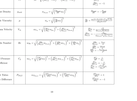
Table 3.1 Definitions and equations for various flow properties . . . 16

Table 3.2 Equations for uncertainty analysis . . . 20

Table 3.3 Scanivalve multi-point electronic pressure-scanning (ESP) module specifications 21 Table 3.4 Given constants . . . 21

Table 3.5 Single Measurement Uncertainties . . . 22

Table 3.6 Flow Condition and Pressure Uncertainties . . . 22

Table 4.1 Pitot-static tube pressure measurements . . . 24

Table 4.2 Onset of flow separation based on surface pressure distributions . . . 29

(9)

LIST OF FIGURES

Figure 1.1 Boundary layer velocity profiles. . . 2

Figure 2.1 Pitot tubes on the airfoil outside the separated regime at low angles of attack and within the separation regime at high angles of attack. . . 7

Figure 3.1 Pitot tubes specifications. . . 9

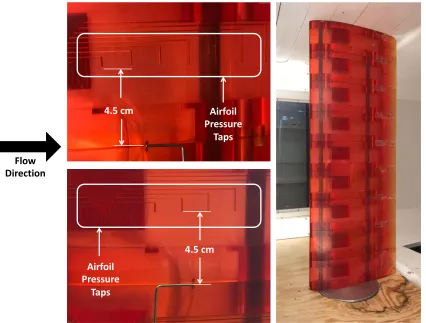
Figure 3.2 Pitot tubes mounted on the airfoil surface at 50% chord location. Forward-facing probe (top), Backward-Forward-facing probe (bottom). . . 10

Figure 3.3 North Carolina State University Subsonic Wind Tunnel [34]. . . 11

Figure 3.4 (Left) Location of the forward and backward-facing pitot tubes with respect to the airfoil pressure taps. (Right) Airfoil model used for mounting the pitot tubes. . . 14

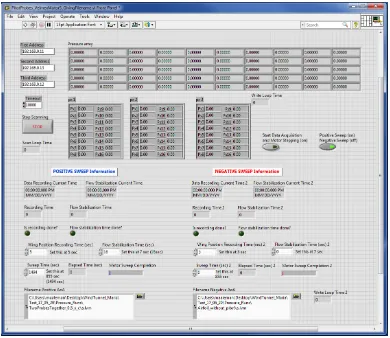
Figure 3.5 A screen shot of the LabVIEW virtual instrument (VI) used for the auto-mated data-acquisition process. . . 15

Figure 3.6 AirfoilCl precision uncertainty. Error bars at 95% confidence intervals. . . . 23

Figure 4.1 q∞ = 5 psf. Pressure coefficient Cp distributions. . . 26

Figure 4.2 q∞ = 8 psf. Pressure coefficient (Cp) distributions. . . 27

Figure 4.6 q∞ = 5 psf. (a)Cl vs. angle of attack (b)Cl precision error with error bars at 95% confidence intervals. . . 30

Figure 4.9 Case 1, q∞ = 5 psf. Pressure (psf) versus AoA (deg) at 50% chord (x/c). (a) forward facing probe (PF), (b) backward-facing probe (PB), and (c) the pressure difference between the forward and backward facing probe (PF -PB). The vertical dashed line represents the AoA at which flow separates at 50% chord based on the experimental pressure distribution over the airfoil. P∞ is the freestream static pressure. Error bars at 95% confidence intervals. . 34

(10)

Figure 4.11 Pressure (psf) versus AoA for cases 1–3 at 50% chord (x/c). (a) Forward-facing probe (PF), (b) backward-facing probe (PB), and (c) pressure

differ-ence between the forward and backward facing probes (PF - PB). The AoA

at which flow separates at 50% chord based on the experimental pressure distribution over the airfoil is denoted with a vertical dashed line color coded with its corresponding case. P∞ is the freestream static pressure. Error bars at 95% confidence intervals. . . 37 Figure 4.12 Pressure difference (PF - PB) zero reference crossing for cases 1–3 at 50%

chord. The AoA at which flow separates at 50% chord based on the experi-mental pressure distribution over the airfoil is denoted with a vertical dashed line color coded with its corresponding case. . . 38 Figure 4.13 (a) Cl versus angle of attack curve, (b) Airfoil Cp distribution at stall (13.5

degrees). . . 39 Figure 4.14 Case 1, q∞ = 5 psf. Pressure (psf) versus AoA (deg) at 60% chord (x/c).

(a) forward facing probe (PF), (b) backward-facing probe (PB), and (c) the

pressure difference between the forward and backward facing probe (PF

-PB). The vertical dashed line represents the AoA at which the stall onset

occurs based on the experimental pressure distribution over the airfoil. P∞ is the freestream static pressure. Error bars at 95% confidence intervals. . . . 40

(11)

Chapter 1

Introduction

Aircraft generally operate in the linear regime of aerodynamics. In this region, the flow is mostly attached and the boundary layer is thin. This results in a linear relation between lift and angle of attack and has been widely studied by a variety of experimental, computational, and analytical methods. As the angle of attack is increased, the adverse pressure gradient on the upper surface and the wall shear cause the flow to lose momentum leading to boundary-layer separation [1,2]. The flow separation progresses towards the leading edge of the wing as the angle of attack is further increased, thereby causing stall, which is characterized by a noticeable loss in lift, a significant increase in drag, and is often associated with loss of control.

(12)

1.1 Flow Separation and Stall

As flow passes over an airfoil, the airfoil experiences a pressure gradient on its upper surface. That pressure gradient exhibits a portion of high to low pressure near the leading edge (LE) region, called a favorable pressure gradient, and the suction peak is the value of the lowest pressure. After the suction peak, the pressure increases in the flow direction and attempts to return to approximately the freestream static pressure. This resultant pressure gradient is called an adverse pressure gradient. There are two necessary factors that cause flow separation, one is the increasing pressure in the flow direction (adverse pressure gradient), and the other is the laminar or turbulent viscosity effects [3]. The flow in the boundary layer suffers a greater deceleration due to the viscosity effects, which reduces the momentum of flow near the wall, and it limits the ability of air to move forward against the pressure [3]. At the onset of separation both the velocity gradient and the shear stress are zero, and at a point downstream of separation flow reversal occurs due to the viscous effects. Figure 1.1 shows the velocity profile inside the boundary layer before the separation point, at the onset of separation, and once flow has separated.

(13)

When the flow is attached to the surface of an airfoil, the airfoil can produce high lift and low drag. However, when the angle of attack is increased, the flow on the upper surface of the airfoil separates due to a high adverse pressure gradient and the stream structure over the upper surface is no longer the most optimum for the best performance. The higher the angle of attack, the more the separated flow region shifts towards the LE and the more it increases in size. The consequence of separated flow at a high angle of attack is a large loss in lift and a significant increase in drag, which are the conditions at which the airfoil is said to be stalled [4]. There exists a close relationship between flow separation and stall, and several modern low-order methods use flow separation as a central element in predicting the loss of lift and stall at high angles of attack [5]. Due to this relationship, knowledge of the separation point is an important element of stall detection and avoidance. The critical flow feature associated with flow separation is the reversal of flow direction at the airfoil surface, which is also accom-panied by a change in direction of shear stress. At the exact location of flow separation, the flow speed at the airfoil surface parallel to the wall becomes zero. Numerous sensors based on different transduction mechanisms can successfully capture the changes in the flow direction and effectively identify the critical aerodynamics flow features like separation-point location, flow reattachment, and stagnation point. For instance, researchers have developed shear-stress sensors based on anemometric principle [6]. Hot-wire sensors [7], thermal flow sensors [8] and hot-film sensors [9, 10] have been demonstrated by researchers to be successful means of sensing flow features. Self-governing smart plasma slats have been developed for sensing and controlling flow separation and incipient wing stall [11, 12].

(14)

identi-wind tunnel setup using optical transduction [18]. Although optical measurement techniques have shown potential in laboratory investigations, the technology is still not entirely feasible for practical applications on aircraft wings due to the complicated camera setup required.

Direct conversion of pillar deflection to electrical output is a more practical approach and these techniques have been explored by exploiting the electromechanical behavior of smart ma-terial systems, such as carbon nanotube arrays [19–21] and piezoelectric microstructures [22,23]. More complicated sensor designs and transduction mechanisms involve cylindrical microstruc-tures attached on flexible platforms [24–26], where the rotational moment of the base of the pillar displaces the membrane underneath due to the influence of external force, to induce a detectable electrical response in the form of capacitance, inductance or resistance change.

The boundary-layer separation is also reflected as a flat-lining in the surface pressure distri-butions as the suction pressure drops to low values resulting in the loss of lift. Surface-pressure signatures have been studied by researchers to identify the connection of boundary-layer be-havior with surface pressures [27,28]. Tracking the surface pressures at different chord locations can also serve as a useful tool for the identification of flow separation and stall detection as adopted by Yeo et al. [29, 30]; in their work, differential pressures at several chordwise locations on the airfoil were monitored, and the relative differences between pressure measurements from the leading-edge and trailing-edge regions were compared against each other, allowing a degree of stall prediction.

1.2 Research Objectives

(15)

measurements characteristic of separation-point location. With some knowledge of the type of airfoil under consideration, the location of the pitot probes can be carefully determined such that the stall angle coincides with the flow separation at the device location. Hence, the knowledge of separation-point crossing the location of the pitot probes can be effectively used as a stall-warning technique. With further development, this system has the promise to lead to the future possibility of developing an entirely self-contained device that can be externally mounted on any aircraft system.

1.3 Outline of Thesis

(16)

Chapter 2

Concept

A pitot probe mounted on the airfoil surface and facing the incoming attached flow will measure the total pressure, i.e. a sum of the local dynamic pressure (depending on the location of the probe within the boundary layer) and the local static pressure corresponding to the surface pressure on the airfoil at that chord location. The total pressure inside the region of separated flow is generally significantly lower than that outside the region, where the pressure is com-parable to the freestream total pressure. The same pitot probe inside a separated-flow regime will register a reduced dynamic pressure due to flow reversal and low static pressure. So, as the angle of attack of the airfoil increases, a surface-mounted pitot probe is expected to observe a drop in the pressure measurements. A critical value of the pressure sensed by the probe can be identified as the onset of flow separation, and this value will correspond to the static pressure on the airfoil at that chord location. Figure 2.1a shows a sketch of a forward-facing probe mounted on the upper surface of an airfoil at 50% chord at an angle of attack of zero degrees, and an image of the same forward-facing probe mounted on the upper surface of an airfoil at an angle of attack of 20 degrees.

(17)

(a) Forward-facing pitot tube (b) Backward-facing pitot tube

Figure 2.1: Pitot tubes on the airfoil outside the separated regime at low angles of attack and within the separation regime at high angles of attack.

thereby requiring the knowledge of the freestream dynamic pressure for normalization. This calls for a pitot-static probe at a different location that is either always facing the freestream or requires necessary corrections to compensate for angle of attack change. Although such a procedure will work, this defeats the idea of having a single, self-sufficient unit mounted externally on the airfoil surface which can detect stall for any freestream condition and without any prior calibration or external sensor knowledge.

(18)

Chapter 3

Experimental Setup

The forward-facing and backward-facing pitot probes were mounted on the upper surface of a low-Reynolds number airfoil, and tests were conducted in the subsonic wind tunnel at North Carolina State University (NCSU). Probe specifications, wind-tunnel facility, test setup, and uncertainty analysis are presented in the following sections.

3.1 Probe Specifications

(19)

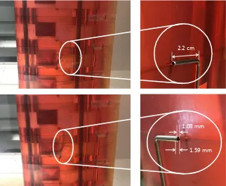
was chosen to be larger than approximately three times the diameter of the stainless steel tubes to minimize any interference [33] caused due to the 90 degrees bend of the probe itself. Figure 3.2 shows the pitot tubes mounted on the airfoil at 50% of the chord.

Side View

OD = 1.59 mm

2.2 cm or 22.0 mm

(a)

Bo#om View

Front View

Distance above airfoil wall

is 0 mm Airfoil Wall

2.2 cm or 22.0 mm

ID = 1.08 mm OD = 1.59 mm t = 0.254 mm

(b)

(20)

1.08 mm

1.59 mm 2.2 cm

Figure 3.2: Pitot tubes mounted on the airfoil surface at 50% chord location. Forward-facing probe (top), Backward-facing probe (bottom).

3.2 Wind-Tunnel Setup

(21)

from experiments performed by fellow a PhD student using a hot-wire anemometer placed at the center of the test section and traversed horizontally ± 20 cm across the test section. At each location tested, the turbulence intensity was determined to be 1.3%. The turbulence intensity is equivalent to the ratio of the root mean square of the velocity fluctuations to the average velocity [35]. The tunnel turbulence factor was calculated using a turbulence sphere test according to the methods described by Barlow and Pope [36], and it was found to be 1.4. An 8-inch diameter sphere was utilized and the tunnel speed was varied in order to obtain measurements at different Reynolds numbers. The high turbulence intensity in this facility increases the chance of having a premature transition from laminar to turbulent flow on the airfoil [36]. This is critical for laminar flow airfoils, especially when attempting to detect flow separation. In order to decrease the need for low turbulence levels it is suggested to install a trip strip near the model’s leading edge to fix the transition point on the model [36]. However, a trip strip was not installed on the model used in this exploratory study, but it is being considered for a follow-on extension.

Figure 3.3: North Carolina State University Subsonic Wind Tunnel [34].

(22)

and a 20% chord trailing edge flap. The flap was maintained at zero degrees deflection for the current work. The airfoil was mounted vertically and the sections were assembled together to span the entire test section from the floor to the ceiling. This configuration simulates a 2-D airfoil by eliminating any tip interference in the test. Each of the sections was fabricated using stereolithography and has pressure ports on the surface along the entire chord length. There are 22 pressure taps on each surface of the airfoil. The taps are unequally spaced around the airfoil so as to obtain more detailed pressure distribution near the leading edge. These taps are able to communicate the instantaneous pressure values to the measurement system via urethane pressure tubing that runs within the airfoil and connects to the wind-tunnel data-acquisition setup. The pressure measurement system consists of three Scanivalve multi-point electronic pressure-scanning (ESP) modules. Each unit is a DSA3217 digital sensor array that incorporates 16 temperature-compensated piezoresistive pressure sensors, and for a sensor pressure range of

±10 inch H2O its static accuracy (% F.S) is ±0.20% (±52.02 psf± 0.20%).

(23)

a rate of 100Hz for 5 seconds, which resulted in 500 data points per pressure tap/probe being recorded at each angle of attack. Once a run was complete, a MATLAB program was used to identify sections of the data corresponding to each angle of attack, and then calculate the mean and the standard deviation of the measurements. The reduced data from the pitot tubes was then plotted for inspection, and the airfoil surface pressures were reduced to pressure coefficients using the tunnel dynamic pressure, which were subsequently integrated using the trapezoid method to calculate the airfoil lift coefficient (Cl). It is worth noting that drag data was not

collected in the current work because it was not essential to predict airfoil flow separation and/or stall at different chord locations.

Flow Direction

4.5 cm Airfoil

Pressure Taps

4.5 cm Airfoil

Pressure Taps

(24)

Figure 3.5: A screen shot of the LabVIEW virtual instrument (VI) used for the automated data-acquisition process.

(25)

separate freestream dynamic pressure measurements were obtained using a pitot-static tube placed at the center of the test section and connected to the wind-tunnel data-acquisition setup. The freestream dynamic pressure measurements taken with the pitot-static tube do not account for the change in freestream dynamic pressure due to the tunnel temperature increase during the time span of each run. The ambient temperature was measured using an Omega Type T Thermocouple that was mounted right after the the two stainless steel anti-turbulence screens, and connected to an Omega 1/8 DIN Thermocouple and RTD Panel Meter Series DP25B.

The equations used to calculate flow conditions, airfoil Cp distribution, and pitot tubes

pressure difference are shown in Table 3.1

Table 3.1: Definitions and equations for various flow properties

Property Symbol Equation

Dynamic Pressure q∞ q∞=Pt,∞−Ps,∞

Ambient Density ρamb ρamb = P_RTamb

Dynamic Viscosity µ µ=µ0

T T0

3/2

T0+S

T+S

Freestream Velocity V∞ V∞=

q

2q∞

ρamb

Reynolds Number Re Re= ρambcV∞

µ

Airfoil Pressure Coefficient Cp Cp = P−_qP_∞s,∞

Pitot Tubes Pressure Difference PDif f PDif f =PF −PB

(26)

the freestream velocity in the test section derived from Bernoulli’s incompressible equation and conservation of mass,cis the airfoil chord,P is the airfoil surface pressure at a particular static port, P∞ is the freestream static pressure, andPF and PB are the pressures measured by the

forward- and backward-facing pitot tubes respectively.

3.3 Zero Angle Of Attack Validation

XFOIL [38] is an analysis and design computational software used for subcritical airfoils. XFOIL uses an inviscid linear-vorticity panel method with a two-equation lagged dissipation integral method that is used to represent the laminar and turbulent layers, and it is coupled with an e9-type amplification formulation to determine the transition point. The implementation of a global Newton method aids in computing the viscous performance of the airfoil. This computational method has proven to be effective in the rapid analysis of low Reynolds number airfoil flows including those with transitional separation bubbles [38]. The XFOIL boundary layer formulation is well founded for attached flows or for a thin separated boundary layer. Therefore, XFOIL predictions are anticipated to be unreliable beyond stall. In addition, previous work done by Gopalarathnam et al [39] showed that in comparison to wind tunnel results, XFOIL tends to over-predict theClmax, stall angle of attack (αstall), and Cl values at angles of

attack close to stall.

(27)

3.4 Data Correction

When a lifting airfoil is in a flow that is constricted between wind tunnel walls, the experimental measurements may not always compare to the airfoil’s performance in free-air. The alteration in the experimental pressure and lift coefficient measurements happen because of blockage and a distortion of the streamlines [40]. There are various correction techniques for airfoil surface pressures and lift coefficient measurements such as the ones discussed by McAlister et al [40]. However, no corrections were made to the data obtained in the present work due to the primary focus being the development of a system to detect flow separation and/or stall, instead of characterizing the airfoil.

3.5 Uncertainty Analysis

Experimental measurements have a certain degree of uncertainty due to the total error given by the instrument. The total error consists of precision and bias error. Precision or random errors are caused by unknown sources that affect the measurements, and are non-repeatable. A way to reduce precision errors is to average multiple sample sets. Contrarily, bias errors are repeatable and caused by known sources such as incorrect calibration and over/under estimation of measurements. Uncertainties in the experimental flow condition, airfoil Cp distribution, and

pitot tubes were calculated using the Kline McClintock method [41], which accounts only for bias uncertainties. Precision and wind tunnel corrections uncertainties are not accounted for.

Assume product R is a function of the independent variables x1, x2, x3, ..., xn, and it is

(28)

wR= s ∂R ∂x1 w1 2 + ∂R ∂x2 w2 2 + ∂R ∂x3 w3 2 +...+ ∂R ∂xn wn 2 (3.2)

where wr is the uncertainty in product R, and w1, w2, w3, ..., wn are uncertainties in the

in-dependent variables that make up product R. Using this method, the flow condition, airfoil

Cp distribution, and pitot tube measurements uncertainties are calculated using the equations

(29)

Table 3.2: Equations for uncertainty analysis

Property Symbol Uncertainty Equation Partial Derivatives

Dynamic Pressure q∞ wq∞ =

r

∂q∞

∂Pt,∞wPt,∞

2

+ ∂q∞

∂Ps,∞wPs,∞

2

∂q∞

∂Pt,∞ = 1

∂q∞

∂Ps,∞ =−1

Ambient Density ρamb wρamb =

r

∂ρamb

∂T wT

2

∂ρamb

∂T =− Pamb

RT2

Dynamic Viscosity µ wµ=

r

∂µ ∂TwT

2

∂µ ∂T =

µ0(S+T0)(3S+T)

√

T /T0

2T0(S+T)2

Freestream Velocity V∞ wV∞ =

r

∂V∞

∂q∞wq∞

2

+

∂V∞

∂ρambwρamb

2

∂V∞

∂q∞ =

√ 2 2ρamb

√

q∞ρamb

∂V∞

∂ρamb =−

√ 2q∞

2(ρamb)2

√

q∞/ρamb

Reynolds Number Re wRe=

r

∂Re ∂ρambwρamb

2

+

∂Re ∂V∞wV∞

2

+

∂Re ∂µ wµ

2

∂Re ∂ρamb =

V∞c

µ ∂Re

∂V∞ =

cρamb

µ ∂Re

∂µ =−

V∞cρamb

µ2

Airfoil Pressure Cp wCp = r

_∂C

p

∂P wP

2

+ ∂Cp

∂Ps,∞wPs,∞

2

+∂Cp

∂q∞wq∞

2 _∂C

p

∂P =

1

q∞

Coefficient ∂Cp

∂Ps,∞ =−

1

q∞

∂Cp

∂q∞ =

−P+Ps,∞

(30)

The Scanivalve multi-point electronic pressure-scanning (ESP) module specifications are listed in Table 3.3.

Table 3.3: Scanivalve ESP module specifications.

Scanivalve Ethernet Pressure Scanner DSA3217 Property Values Units Static Accuracy (% Full Scale)

Range ±5 inch H2O ±0.40%

±10 inch H2O ±0.20%

±1 psid ±0.12%

±2.5 psid ±0.08%

±5 to 500 psid ±0.05%

±501 to 750 psid ±0.08%

15 to 250 psia ±0.05% (with calibration performed) 15 to 250 psia ±0.10% (without calibration performed)

(including linearity, hysteresis, and repeatability)

The Scanivalve ESP modules utilized for data acquisition had a pressure range of±10 inch H2O, which is equivalent to ±52.02 psf with relative and absolute uncertainties of±0.20% and

±0.1040 psf respectively. Let’s consider an example test case to perform uncertainty analysis:

the 12%-thick low-Reynolds-number airfoil tested at a Reynolds number of 0.39 million and angle of attack of 6 degrees. For the example test case, the constants used for the uncertainty analysis are shown in Table 3.4 and the single measurement uncertainties are shown in Table 3.5. Table 3.6 shows the calculated flow condition and pressure uncertainties for the example test case.

Table 3.4: Given constants

Property Units Value

Airfoil Chord (c) ft 1

Gas Constant (R) fl-lb/(slug-deg R) 1716 Reference Temperature (T0) deg R (K) 491.6 (273.11) Sutherland Temperature (S) deg R (K) 199.8 (110.56) Reference Dynamic Viscosity (µ0) lb-s/ft2 3.58E-7

(31)

Table 3.5: Single Measurement Uncertainties

Property Units Reference Absolute Relative

Value Uncertainty Uncertainty

Ambient Temperature (T) F (R) 72 (531.67) ±0.9 (±0.9) ±1.25% (±0.17%) Freestream Static (Ps,∞) psf 0.09 ±0.1040 ±115.60% Pressure

Freestream Total (Pt,∞) psf 4.9 ±0.1040 ±2.12% Pressure

Pitot Forward-Facing (PF) psf 1.4 ±0.1040 ±7.43%

Pressure

Pitot Backward-Facing (PB) psf -4.05 ±0.1040 ±2.59%

Pressure

Airfoil Surface Pressure (P) psf -5.756 ±0.1040 ±1.81%

Table 3.6: Flow Condition and Pressure Uncertainties

Property Units Reference Absolute Relative

Value Uncertainty Uncertainty Freestream Dynamic Pressure (q∞) psf 4.81 ±0.1471 ±3.06% Ambient Density (ρamb) slug/ft3 0.0023 ±3.8915E-6 ±0.17%

Dynamic Viscosity (µ) lb-s/ft2 3.8059E-7 ±4.9811E-10 ±0.13%

Freestream Velocity (V∞) ft/s 64.69 ±0.99 ±1.53%

Reynolds Number (Re) - 390736 ±6043 ±1.55%

Airfoil Pressure Coefficient (Cp) - -1.215 ±0.048 ±3.96%

Pitot Pressure Difference (PDif f) psf 5.45 ±0.15 ±2.70%

Airfoil Cl uncertainties were not calculated using the Kline McClintock method due to its

complexity. Instead, precision uncertainties were calculated by integrating the Cp distribution

data to obtain Cl values, and then the mean and standard deviation of the Cl values was

calculated. The confidence interval was set at 95% (2σ). The Cl precision uncertainty for the

(32)

(33)

Chapter 4

Results

This chapter presents the results from the tests conducted in the subsonic wind tunnel at North Carolina State University. The results from the pitot-static tube pressure measurements, flow separation prediction obtained from the airfoil Cp distribution, airfoil lift curve, and

flow-separation and stall detection using the surface-mounted pitot-tubes are discussed in the fol-lowing sections.

4.1 Pitot-Static Tube Measurements

The results for the pitot-static pressure measurements taken at the center of the test section for three freestream dynamic pressure cases (5, 8, and 10 psf) are presented in Table 4.1.

Table 4.1: Pitot-static tube pressure measurements

Tunnel Dynamic Pressure Mean Absolute Relative

Pressure (psf ) Type Pressure (psf ) Uncertainty (psf ) Uncertainty

5 Total 4.9201 ±0.1040 ±2.11%

Static 0.0823 ±0.1040 ±126.37%

8 Total 7.9780 ±0.1040 ±1.30%

(34)

The freestream total pressure measured by the pitot-static tube is equal to the total pres-sure minus the atmospheric prespres-sure, which is equivalent to the tunnel dynamic prespres-sure. And the measured freestream static pressure is equal to the static pressure minus the atmospheric pressure, which should be a value close to zero.

4.2 Airfoil Surface Pressure Distributions And Lift Curve

4.2.1 Flow Separation Prediction From Cp Distribution

The pressure gradient on the upper surface of an airfoil changes with angle of attack. As the angle of attack is increased, the pressure gradient becomes more adverse or less favorable on the upper surface, representing an increase in pressure in the flow direction (positivedP/dx). At low angles of attack, the pressure at the trailing edge reaches a value minimally higher compared to the freestream static pressure, but at high angles of attack the pressure near the trailing edge becomes smaller than the freestream static pressure [4] and a constant pressure region is originated. The chordwise location where the pressure plateau meets the start of the adverse pressure gradient serves as an indicator of the location of the onset of flow separation. This behavior was looked for in the Cp distributions at different angles of attack to determine the

onset of flow separation at three different chordwise locations (50%, 60%, and 70% chord). The angles of attack at which the surface pressure distributions reflected the onset of flow separation at 50%, 60%, and 70% chord were used to corroborate the predictions from the pitot tubes.

(35)

Figures 4.1b, 4.2b, 4.3b show the location of the onset of separation slightly downstream and upstream of the 50% chord location. The surface pressure distributions reflecting the location of the onset of separation slightly downstream and upstream of the 60% and 70% chord locations at a freestream dynamic pressure of 5 psf are shown in Figures 4.4 and 4.5.

Separa&on at 52.70%-chord

(a) AoA = 14.5 degrees

(b) AoA = 15 degrees

(36)

Figure 4.2: q∞= 8 psf. Pressure coefficient (Cp) distributions.

(37)

(38)

Table 4.2: Onset of flow separation based on surface pressure distributions

Chordwise Location Tunnel Dynamic Pressure (psf ) Angle of Attack (deg)

50% 5 14.5

8 14.8

10 14.8

60% 5 13.8

70% 5 12.9

4.2.2 Lift Coefficient Versus Angle of Attack Curve

The Cl versus angle of attack curves from experiments at three different freestream dynamic

pressures can be seen in Figures 4.6a, 4.7a, and 4.8a. The predicted curves obtained from XFOIL computations are also shown in these figures. It is seen that for angles of attack greater than 8 degrees, XFOIL over-predictsCl compared to the experimental values, which is expected for

angles of attack close to and beyond stall, as mentioned in Section 3.3. However, for the 5, 8, and 10 psf freestream dynamic pressure cases the stall angle of attack was 13.5, 14, and 14.5 degrees respectively, thus experimentalClvalues between 8 degrees and the stall angles of

attack are slightly less compared to XFOIL. In addition, the linear slope of theCl versus angle

of attack curve does not match entirely between the computational and experimental results. These discrepancies could be attributed to test setup influences, wind tunnel turbulence levels, and not applying correction factors. Some of the test setup influences are errors in the zero angle of attack location, the model’s placement not being at the center of the test section, and the clearance size between the model and the test section’s roof. The model was placed far back in the test section and the trailing edge was approximately 3 cm away from the test section’s gap, where air is suctioned, which could have allowed for 3D effects (spanwise flow). When the clearance size between the model and the test section top was very small, the leading edge dragged at the top of the test section, making it difficult for the Velmex stepping motor to rotate the model to the correct angle of attack. These test setup influences were recognized at a late stage and were not resolved due to time constraints.

(39)

in Figures 4.6b, 4.7b, and 4.8b respectively. For all three cases, theClvalue limits are very close

to the meanCl values for angles of attack from zero to the stall angle of attack, and for angles

of attack beyond stall the fluctuations inClvalues increase. This is expected since surface static

pressure is likely to start deviating as the separated flow region increases.

(a) (b)

Figure 4.6: q∞= 5 psf. (a)Cl vs. angle of attack (b)Clprecision error with error bars at 95%

(40)

(a) (b)

Figure 4.7: q∞= 8 psf. (a)Cl vs. angle of attack (b)Clprecision error with error bars at 95%

confidence intervals.

(a) (b)

Figure 4.8: q∞ = 10 psf. (a) Cl vs. angle of attack (b) Cl precision error with error bars at

(41)

4.3 Pitot-Tubes Tests

Wind-tunnel tests were performed for three different freestream dynamic pressures, as listed in Table 4.3. For each case, separate runs were conducted with the pitot tubes at three different chordwise locations (50%, 60%, and 70% chord) on the upper surface of the airfoil.

Table 4.3: Cases with the forward and backward-facing pitot probes placed separately at 50% chord and 70% chord on the airfoil upper surface.

Case Reynolds Freestream Tunnel Dynamic

Number Number Velocity (m/s) Pressure (psf )

1 0.39 million 20 5

2 0.5 million 24 8

3 0.56 million 28 10

4.3.1 Flow Separation Detection

The results for case 1, where the freesteam dynamic pressure is 5 psf, are presented in Figures 4.9 and 4.10. In this run, the pitot probes were mounted on the upper surface of the airfoil at 50% chord location. The mean and the standard deviation of the pressures recorded by the pitot probes at each angle of attack are plotted in the results.

Figure 4.9a shows the measurements made by the forward-facing pitot probe (PF). This

(42)

approaches the probe location, unsteady flow structures are sensed by the pressure sensors resulting in greater fluctuations in the recorded data.

The backward-facing pitot probe measurements (PB) were compared to the static pressure

measurements at the 50% chord location. The results display a trend that is close to the local static pressure, as shown in Figure 4.9b. The pressure measured by the backward-facing probe was expected to be close to the local static pressure except for some deviation due to the probe wake, as mentioned in Section 2.

The results from the pressure difference between the forward- and backward-facing probes (PF - PB) exhibit a decreasing trend as shown in Figure 4.9c. The pressure difference reaches

zero at an angle of attack of 15.5 degrees which suggests the onset of the separation at the probe location. This was confirmed by the observing the flat-lining or the development of a constant pressure region in the surface pressure distribution on the airfoil, as mentioned in the Section 4.2.1. The surface pressure distribution reflected the onset of flow separation at 50% of the chord for the angle of attack of 14.58 degrees. The prediction from the pitot probes is within 1 degree of the estimated angle of attack using the surface pressures. The slight over-prediction could be attributed to the interference caused due to the probes themselves. Overall, the estimate is reasonable and the results prove that the pitot-probe system has the potential to detect the onset of flow separation at the probe location.

(43)

(a) (b)

(c)

Figure 4.9: Case 1, q∞ = 5 psf. Pressure (psf) versus AoA (deg) at 50% chord (x/c). (a) forward facing probe (PF), (b) backward-facing probe (PB), and (c) the pressure difference

between the forward and backward facing probe (PF -PB). The vertical dashed line represents

(44)

(a) (b)

(c)

between the forward- and backward-facing probe (PF -PB). The vertical dashed line represents

(45)

4.3.2 Effect of Freestream Dynamic Pressure

(46)

(a) (b)

(c)

Figure 4.11: Pressure (psf) versus AoA for cases 1–3 at 50% chord (x/c). (a) Forward-facing probe (PF), (b) backward-facing probe (PB), and (c) pressure difference between the forward

and backward facing probes (PF - PB). The AoA at which flow separates at 50% chord based

(47)

Figure 4.12: Pressure difference (PF - PB) zero reference crossing for cases 1–3 at 50% chord.

The AoA at which flow separates at 50% chord based on the experimental pressure distribution over the airfoil is denoted with a vertical dashed line color coded with its corresponding case.

4.3.3 Stall Detection

Based on the results, it is clear that separation point reaches 70% chord at an angle of attack of 14 degrees and the separation further moves till 50% when the angle of attack has been increased to 15.5 degrees. The next step is to correlate the location of separation point with the airfoil stall angle of attack. To study that relationship, the coefficient-of-pressure (Cp) distribution was

integrated to calculate the lift coefficient (Cl) and determine the stall angle. The stall angle of

(48)

(a)

(b)

Figure 4.13: (a) Cl versus angle of attack curve, (b) Airfoil Cp distribution at stall (13.5 degrees).

(49)

(a) (b)

(c)

between the forward and backward facing probe (PF -PB). The vertical dashed line represents

(50)

Chapter 5

Conclusions and Future Work

5.1 Conclusions

(51)

The results presented in this thesis demonstrate the capability of a two-probe system to capture the onset of flow separation at the probe location irrespective of the freestream velocity. For any airfoil, the location of the separation-point on the surface can be correlated with the stall angle. Hence, the knowledge of the separation-point location obtained from the pitot probes can be effectively used for stall detection and avoidance. These results support the possibility of a completely self-sufficient device comprising of the opposite-facing pitot tube system similar to that used in this research.

5.2 Future Work

A next step in research would be to make slight changes to the setup and perform oil flow visualization to characterize the low-Reynolds number airfoil used in this work. This would be done to eliminate the errors in the Cl values at low angles of attack, and to check the

(52)

(a) 3D Prototype.

Front orifice Back orifice _{(opposite to flow} direc4on)

(b) 3D Prototype inside view.

Front orifice Back orifice _{(opposite to flow direc4on)}

(c) Prototype inside view.

Front oriﬁce Back oriﬁce

(opposite to ﬂow direc4on)

(53)

REFERENCES

[1] Dennis M. Bushnell and Mohamed Gad-el Hak. Separation control: review. Journal of fluids engineering, 113:5, 1991.

[2] R.L. Simpson. Review-a review of some phenomena in turbulent flow separation. ASME Journal of Fluids Engineering, 103:520–533, 1981.

[3] Paul K. Chang. Separation of Flow. Pergamon Press Ltd., 1st edition, 1970.

[4] John D. Anderson Jr. Fundamentals of Aerodynamics. McGraw-Hill, 5th edition, 2010.

[5] Joaquim N Dias. Nonlinear lifting-line algorithm for unsteady and post-stall conditions. AIAA Paper 2016-4164, June 2016.

[6] Chang Liu, Jin-Biao Huang, Zhenjun Zhu, Fukang Jiang, S. Tung, Yu-Chong Tai, and Chih-Ming Ho. A micromachined flow shear-stress sensor based on thermal transfer principles. Journal of Microelectromechanical Systems, 8(1):90–99, Mar 1999.

[7] Ulrich Buder, Ralf Petz, Moritz Kittel, Wolfgang Nitsche, and Ernst Obermeier. Aeromems polyimide based wall double hot-wire sensors for flow separation detection. Sensors and Actuators A: Physical, 142(1):130 – 137, 2008. Special Issue: Eurosensors{XX} The 20th European conference on Solid-State TransducersEurosensors 2006Eurosensors 20th Edi-tion.

[8] Dieter Westermann Hannes Sturm, Gerrit Dumstorff and Walter Lang. Boundary layer separation and reattachment detection on airfoils by thermal flow sensors. Journal of Sensors, 2012.

(54)

[10] T Lee and S Basu. Measurement of unsteady boundary layer developed on an oscillating airfoil using multiple hot-film sensors. Experiments in Fluids, 25(2):108–117, 1998.

[11] Mehul P Patel, Zak H Sowle, Thomas C Corke, and Chuan He. Autonomous sensing and control of wing stall using a smart plasma slat. Journal of aircraft, 44(2):516–527, 2007.

[12] Thomas C. Corke, Patrick O. Bowles, Chuan He, and Eric H. Matlis. Sensing and control of flow separation using plasma actuators. Philosophical Transactions of the Royal Society of London A: Mathematical, Physical and Engineering Sciences, 369(1940):1459–1475, 2011.

[13] Fukang Jiang, Gwo-Bin Lee, Yu-Chong Tai, and Chih-Ming Ho. A flexible micromachine-based shear-stress sensor array and its application to separation-point detection. Sensors and Actuators A: Physical, 79(3):194 – 203, 2000.

[14] E P Gnanamanickam, B Nottebrock, S Große, J P Sullivan, and W Schr¨oder. Measurement of turbulent wall shear-stress using micro-pillars. Measurement Science and Technology, 24(12):124002, 2013.

[15] Sebastian Große and Wolfgang Schr¨oder. Dynamic wall-shear stress measurements in tur-bulent pipe flow using the micro-pillar sensor mps 3. International Journal of Heat and Fluid Flow, 29(3):830–840, 2008.

[16] Benjamin Dickinson, John Singler, and Belinda A Batten. The detection of unsteady flow separation with bioinspired hair-cell sensors. In 26th AIAA Aerodynamic Measurement Technology and Ground Testing Conference, AIAA Paper 2008-3937, 2008.

[17] Benjamin Dickinson, John Singler, and Belinda A Batten. Mathematical modeling and simulation of biologically inspired hair receptor arrays in laminar unsteady flow separation. Journal of Fluids and Structures, 29:1–17, 2012.

(55)

Aerodynamic flow sensing with elastic microfence structures. In 55th AIAA Aerospace Sciences Meeting, AIAA Paper 2017-0479, 2017.

[19] Gregory J Ehlert, Matthew R Maschmann, and Jeffery W Baur. Electromechanical be-havior of aligned carbon nanotube arrays for bio-inspired fluid flow sensors. In SPIE Smart Structures and Materials+ Nondestructive Evaluation and Health Monitoring, pages

79771C–79771C. International Society for Optics and Photonics, 2011.

[20] C Pozrikidis. Shear flow over cylindrical rods attached to a substrate. Journal of Fluids and Structures, 26(3):393–405, 2010.

[21] D M Phillips, C W Ray, B J Hagen, W Su, J W Baur, and G W Reich. Detection of flow separation and stagnation points using artificial hair sensors. Smart Materials and Structures, 24(11):115026, 2015.

[22] Taeyang Kim, Aditya Saini, Jinwook Kim, Ashok Gopalarathnam, Yong Zhu, Frank L Palmieri, Christopher J Wohl, and Xiaoning Jiang. A piezoelectric shear stress sensor. In SPIE Smart Structures and Materials+ Nondestructive Evaluation and Health Monitoring,

pages 98032S–98032S. International Society for Optics and Photonics, 2016.

[23] D Roche, C Richard, L Eyraud, and C Audoly. Piezoelectric bimorph bending sensor for shear-stress measurement in fluid flow. Sensors and Actuators A: Physical, 55(2):157–162, 1996.

[24] AMK Dagamseh, RJ Wiegerink, TSJ Lammerink, and GJM Krijnen. Towards a high-resolution flow camera using artificial hair sensor arrays for flow pattern observations. Bioinspiration & biomimetics, 7(4):046009, 2012.

(56)

[26] Nannan Chen, Craig Tucker, Jonathan M Engel, Yingchen Yang, Saunvit Pandya, and Chang Liu. Design and characterization of artificial haircell sensor for flow sensing with ultrahigh velocity and angular sensitivity. Microelectromechanical Systems, Journal of, 16(5):999–1014, 2007.

[27] Michael S. H. Boutilier and Serhiy Yarusevych. Parametric study of separation and tran-sition characteristics over an airfoil at low reynolds numbers. Experiments in Fluids, 52(6):1491–1506, 2012.

[28] Yongwei Gao, Qiliang Zhu, and Long Wang. Measurement of unsteady transition on a pitching airfoil using dynamic pressure sensors. Journal of Mechanical Science and Technology, 30(10):4571–4578, 2016.

[29] Derrick Yeo, Joshua Henderson, and Ella Atkins. An aerodynamic data system for small hovering fixed-wing UAS. AIAA Paper 2009-5756, 2009.

[30] Derrick Yeo, Ella M Atkins, Luis P Bernal, and Wei Shyy. Aerodynamic sensing for a fixed wing UAS operating at high angles of attack. AIAA Paper 2012-4416, 2012.

[31] Preston J. H. The determination of turbulent skin friction by means of pitot tubes. Journal of the Royal Aeronautical Society, 58(518):109–121, 1954.

[32] Terry Beck, Greg Payne, and Trevor Heitman. The aerodynamics of the pitot-static tube and its current role in non-ideal engineering applications. In American Society for Engi-neering Education, pages 15.1204.1–16, 2010.

[33] Jose C. Gonsalez Trong T. Bui, David L. Oates. Design and evaluation of a new boundary-layer rake for flight testing. Technical Memorandum 209014, NASA Dryden Flight Research Center, 2000.

(57)

[35] W. C. Mock Jr. Hugh L. Dryden, G. B. Schubauer and H. K. Skramstad. Measurements of intensity and scale of wind-tunnel turbulence and their relation to the critical reynolds number of spheres. Technical Report 581, National Advisory Committee For Aeronautics, 1937.

[36] Alan Pope Jewel B. Barlow, William H. Rae Jr. Low-Speed Wind Tunnel Testing. John Wiley & Sons, INC., 3rd edition, 1999.

[37] Jeffrey K. Jepson and Ashok Gopalarathnam. Experimental demonstration of a sense-and-adapt approach for automated sense-and-adaptation of a wing with multiple trailing-edge flaps. In 25th AIAA Applied Aerodynamics Conference, number AIAA 2007-4062, June 2007.

[38] Mark Drela. XFOIL: An Analysis and Design System for Low Reynolds Number Airfoils. In T. J. Mueller, editor,Low Reynolds Number Aerodynamics, volume 54 ofLecture Notes in Engineering, pages 1–12. Springer-Verlag, New York, June 1989.

[39] Ashok Gopalarathnam and Michael S. Selig. Low-speed natural-laminar-flow airfoils: Case study in inverse airfoil design. Journal of Aircraft, 38(1), January-February 2001.

[40] K. W. McAlister and R. K. Takahashi. NACA 0015 wing pressure and trailing vortex measurements. Technical Report 3151, NASA Ames Research Center, Moffett Field, CA 94035, November 1991.