Comparison of Exact Unconditional Methods for the Difference of Two Binomial Proportions

(1)

Exact tests based upon the difference of two independent binomial proportions are

popularly used and are especially suited for studies with small to moderate sample

sizes. In the context of testing for superiority and noninferiority, we apply the

confi-dence region p-value method (Berger and Boos, 1994) in proposing an exact test that

has been found to perform better than the standard exact test in many situations.

The exact tests use unconditional distributions and the variances of the test statistics

are determined via a restricted maximum likelihood method (Farrington and

Man-ning, 1990). Inverting the tests, we derive corresponding confidence intervals and

we provide coverage probability and expected length comparisons. These

compar-isons show that, in many cases, the confidence intervals based upon the proposed

exact method have less conservative coverage and shorter lengths when compared to

(2)

A dissertation submitted to the Graduate Faculty of North Carolina State University

in partial fulfillment of the requirements for the Degree of

Doctor of Philosophy

STATISTICS

Raleigh

2003

APPROVED BY:

Roger L. Berger William H. Swallow

Chair of Advisory Committee

(3)

(4)

In December of 1995, at California State University Northridge, he received his

Bachelor of Arts degree in Mathematics with minors in Japanese, Biology, and

Chem-istry. In the summer of 1996 he packed up his belongings into his trusty Honda Accord

and drove 2,560 miles eastbound on I-40 towards Raleigh to begin his graduate studies

in the Department of Statistics at North Carolina State University.

In 1998, Jimmy received his Masters of Statistics degree and in 2003 he completed

his Ph.D. in Statistics at NC State. During his time in the graduate program he was

afforded the opportunity to teach undergraduate courses and the experience affirmed

his life long ambition to enter academics to pursue his professional career. In the fall

of 2003, he will join the faculty of the Department of Statistics at Cal Poly San Luis

Obispo.

(5)

been planted with the help of a supporting cast of many, and the work represented

in this manuscript is certainly no exception. My only regret is that I will not be able

to properly express in words the multiple pages of gratitude that each person listed

here surely deserves.

First, I would like to express my sincere appreciation to my advisor Dr. Roger

Berger. I am especially grateful for his incredible patience and understanding. Through

my interactions with him I have learned a great deal not only about research but also

about the academic life and I truly appreciate his steadfast guidance. I would also

like to thank each of the committee members for their valuable input and service.

In terms of the guidance and instruction I have received from the members of the

department, I could not have asked for a better collection of faculty to learn from.

I would like to acknowledge two faculty members in particular: Dr. Sastry Pantula

and Dr. Bill Swallow.

As Director of Graduate Programs for most of my stay, Dr. Pantula has been

an incredible source of support. Whenever I needed to seek guidance, his door was

always open and he was always willing to lend me his ear and offer helpful advice. I am

especially grateful for the manner in which he always “raised the bar of expectation”

and how he always asked for the best of me – I am forever indebted to him for that.

(6)

student, I have had the fortune of many successful teaching experiences which I owe,

at least in part, to him. Being the modest person that he is, Dr. Swallow would

probably be first to disagree with the notion that he taught me how to teach, however

I can say without hesitation that he taught me how to teachbetter.

When I had the opportunity to help recruit graduate students to our department,

one aspect I liked to boast about is the warmth and family-like environment we

enjoy. This congenial atmosphere is surely maintained by, among others, our many

kind and friendly departmental staff. I am thankful for all of the staff members and

I am especially grateful for Ms. Janice Gaddy (Mom). With every question I have

had,Mom looked after my concerns and addressed my needs with the utmost level of

care, efficiency, and professionalism. Without a doubt, she will be one of the people

I will miss most from the program.

Another crucial person of our department I need to thank is our systems

adminis-trator Terry Byron. Terry is quite simply the best. He has helped me in more ways

than I can keep track of and, probably, in more ways than he would like toremember.

I have always appreciated the incredible patience he has extended to me. Many times,

even when he was completely swamped with other work, he cheerfully took the time

to go the proverbial ‘extra mile’ with whatever computer related questions I had and

(7)

our family and friends”. As I look back upon my experience in the program, I find

this to be quite evident and I can honestly say some of my fondest memories stem

from the relationships I have been blessed with over the years. Although I will not be

able to thank everyone properly, I would like to give special thanks to the many

grad-uate students I have befriended and to those brave enough to endure my Japanese

cooking experiments which occurred in my kitchen.

I am particularly grateful for the following friends: Prasheen Agarwal, Jarrett

Barber, Doug Robinson, Abdus Wahed, Kapil Sen, Pralay Mukhopadhyay, Joshua

Tebbs, Zeynep Kalaylioglu, Ross Gosky, Selene Leon, Julie McIntyre, and Alvin Van

Orden. They have all, in their own special ways, helped to make my graduate school

experience a memorable one.

Now, I would be completely remiss if I failed to mention one particular friend

and officemate, Jared Lunceford. The many classes we had together were much

more enjoyable sitting next to that guy, even when he volunteered me to answer

impossible measure theory questions. I have really appreciated his unique humor,

candor, and counsel. Truly, it has been my honor to call upon him as a friend. I

am especially grateful to have had the opportunity to know his wonderful wife Heidi

and their beautiful children. Looking back on my experience in Raleigh, some of the

(8)

integrity. To my mother, I am grateful for the love and wisdom she has imparted

towards me and for being one of my greatest teachers. To my irreplaceable sister

Kathy, I am grateful for her always being there and for the great friendship we enjoy.

To her, I say “Now, it’s your turn girl!”. To my entire family, I especially appreciate

the countless encouragements I have received from them throughout my years in

school. Iro iro taihen osewa ni natte hontou ni arigato gozaimashita!

The Roman statesman Seneca once said “I delight in learning so that I can teach”.

No other statement encapsulates the very motivation which has driven me throughout

my education to reach this point. It has been my lifelong dream to achieve this goal

and now I delight in the wonderful realization that my career in academics is about

to begin.

(9)

List of Tables xv

1 Introduction 1

1.1 Model Formulation . . . 3

1.2 The _δ Projected _Z Statistic . . . 4

1.3 p-value and the Nuisance Parameter Problem . . . 6

1.4 Confidence Region p-value Method . . . 9

2 Comparison of Unconditional Exact Tests for Testing the Difference of Independent Binomial Proportions 12 2.1 Testing for Superiority . . . 13

2.1.1 Introduction . . . 13

2.1.2 Computation Study . . . 14

2.1.3 Examples of _T_p_r Performance Relative to _T_p_u . . . 15

2.1.4 Results . . . 19

(10)

2.2.3 Example of _T_p_r Performance Relative to _T_p_u . . . 42

2.2.4 Results . . . 45

2.2.5 Size Plots for _δ₀ =−0_.10 . . . 59

2.3 Conclusion . . . 63

2.3.1 Superiority Trials . . . 63

2.3.2 Noninferiority Trials . . . 64

3 Comparison of Exact Confidence Intervals for the Difference of Two Binomial Proportions 66 3.1 Introduction . . . 66

3.2 An Efficient Method to Generate (_{x, y}) for Confidence Intervals for _δ 68 3.3 Comparison of the Exact Confidence Intervals . . . 76

3.3.1 Coverage Probability . . . 76

3.3.2 Average Length Comparisons . . . 99

3.3.3 Expected Length Comparisons . . . 106

3.3.4 Relative Difference of Expected Length Comparisons . . . 117

3.4 Conclusion . . . 127

Bibliography 129

(11)

A.2 Computing a Confidence Interval for _δ . . . 135

A.2.1 Case 1: _X =_{x, Y} =_y . . . 135

A.2.2 Case 2: _X =_n₁ −_{x, Y} =_n₂−_y . . . 138

(12)

1.2 (1−_β) confidence region for (_π₁_{, π}₂)∈Θ₀ . . . 11

2.1 Superiority hypothesis spaces as specified by (2.1.2). . . 14

2.2 (_{x, y})∈ R_p_r,(_{x, y})6∈ R_p_u. . . 17

2.3 (_{x, y})∈ R_p_r, (_{x, y})6∈ R_p_u. . . 19

2.4 Size plots for testing_H₀ :_δ≤0_.10 at the _α= 1% level. . . 36

2.7 Size plots for testing_H₀ :_δ≤0_.10 at the_α = 1% level where (_n₁_{, n}₂) = (100_,100). . . 39

2.8 Size plot for _T_p_u testing _H₀ :_δ≤0_.10 at the _α= 1% level. . . 39

2.9 Noninferiority hypothesis spaces as specified by (2.1.2). . . 41

2.10 (_{x, y})6∈ R_p_r, (_{x, y})∈ R_p_u . . . 45

2.11 Size plots for testing _H₀ :_δ≤ −0_.10 at the _α= 1% level. . . 60

2.12 Size plots for testing _H₀ :_δ≤ −0_.10 at the _α= 5% level. . . 61

(13)

at fixed _δ settings. . . 82

3.3 (_n₁ :_n₂) = (1 : 1) case. Coverage probability plots for_n₁ = 50,_n₂ = 50

3.4 (_n₁ :_n₂) = (2 : 1) case. Coverage probability plots for_n₁ = 13, _n₂ = 7

at fixed _π₂ settings. . . 93

(14)

3.14 (_n₁ :_n₂) = (1 : 1) case. Expected length plots for _n₁ = 10, _n₂ = 10 at

fixed_π₂ settings. . . 111

fixed_δ settings. . . 112

3.20 (_n₁ : _n₂) = (1 : 1) case. Relative difference of expected lengths

(_RDEL) for _n₁ = 10, _n₂ = 10 at fixed _π₂ settings. . . 121

(15)

A.1 Confidence region relationship for (_{X, Y}) = (_{x, y}) and (_{X, Y}) = (_x0_{, y}0) =

(_n₁−_{x, n}₂−_y) . . . 136

(16)

2.2 Comparison of rejection regions based on _p_r and _p_u for _H₀ :_δ≤0_.10. 24

2.11 Comparison of rejection regions based on _p_r and _p_u for _H₀ :_δ ≤0_.10,

complete 1:1 case. . . 33

2.12 Comparison of rejection regions based on _p_r and _p_u for _H₀ :_δ≤ −0_.10. 49

(17)

2.21 Comparison of rejection regions based on_p_r and_p_ufor_H₀ :_δ≤ −0_.10,

complete 1:1 case. . . 58

3.1 Association between (_{x, y}) and (_x0_{, y}0) = (_n₁−_{x, n}₂ −_y). . . 70

3.2 Index label and sample point associations. . . 72

3.3 Index label associations for (_{x, y}). . . 72

3.4 Quotient-ratio representations of index values compared to index label associations for (_{x, y}) . . . 74

3.5 Average length comparisons for _p_u versus _p_r where _n₁ :_n₂ = 1:1. . . . 103

(18)

Research for discrete data stemming from clinical trials often relied upon an

asymptotic distribution, as opposed to the true or exact distribution, of the test

statistic of interest. Analyses that rely upon exact distributions usually involve

in-tense computations and so the relatively convenient asymptotic methods offer an

attractive time-saving alternative. Asymptotic methods, by their very nature,

per-form well when sample sizes are large. However, when sample sizes are small to

moderate, as found in many clinical trials, exact methods are preferred. Recently,

exact tests have become popular and more accessible due to the increase in speed and

power of computing resources.

In this work, we will focus upon the analysis of data arising from clinical trials

where the parameter of interest is the difference of two independent binomial

propor-tions. This parameter of interest is often used in the context of testing for superiority

and noninferiority.

(19)

that the conditional distribution of the sample, given _W =_w, is free of the nuisance

parameter. Thus, one can construct an exact test through inference based on this

conditional distribution. One disadvantage of exact conditional tests is that they can

often perform very conservatively (Liddell, 1978, Suissa and Shuster, 1985, Berger,

1996). However, researchers have suggested that, in some contexts, conditional tests

are preferred (Agresti, 1990, Greenland, 1991, Little, 1989, and Yates, 1984).

For reasons we will discuss later, in the general problem of testing for superiority

and noninferiority, non-trivial conditional methods are unavailable. Thus, in our

analyses of these hypothesis tests, we will employ an exact unconditional approach.

The specific problem we must overcome is the presence of a nuisance parameter when

defining a p-value. One popular unconditional approach to address this problem is to

determine the supremum of the p-value function over the entire nuisance parameter

space. This method is often referred to as the maximization method. Although this

method yields a valid p-value, it can be quite conservative. Berger and Boos (1994)

proposed a method to alleviate this conservativeness by applying a restricted nuisance

parameter space search. This is known as the confidence region p-value method.

Before providing the details of both methods, let us first outline the model

for-mulation of the problem and also discuss the particular test statistic we will be using

(20)

Consider a clinical trial where the goal is to compare the efficacy of a new

treat-ment (drug 1) versus that of a standard (drug 2). Let us denote_π₁ and _π₂ as the true

response rates of the new and standard treatments respectively. Often, researchers

compare these two rates through their difference which we will denote as_δ=_π₁−_π₂.

Suppose _X and _Y are independent binomial random variables. The sample size

for_X is_n₁and its success probability is_π₁. The sample size for_Y is_n₂and its success

probability is _π₂. Data stemming from these clinical trials are often summarized in

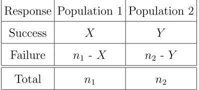
2×2 contingency tables as shown below.

Response Population 1 Population 2

Success _X _Y

Failure _n₁ - _X _n₂ - _Y

Total _n₁ _n₂

Let us denote the binomial probability mass function of _X by

bin(_{x, n}₁_{, π}₁) = µ

n1 x

¶

π1x(1−π1)n1−x, where x= 0,1, . . . , n1.

Denote bin(_{y, n}₂_{, π}₂) as the analogous representation of the probability mass

func-tion of _Y. The sample space of the random vector (_{X, Y}) will be denoted by

Ω ={0_,1_{, . . . , n}₁} × {0_,1_{, . . . , n}₂}.

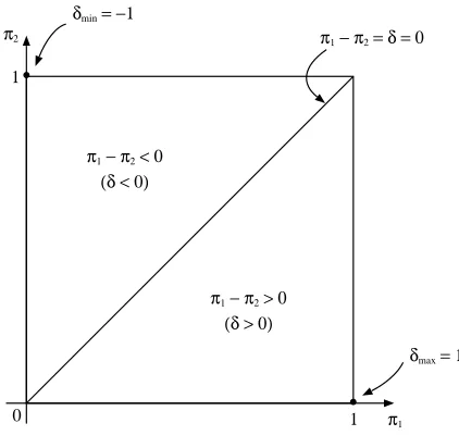
Figure 1.1 is a graphical depiction of the parameter space of (_π₁_{, π}₂). The line

δ=_π₁−_π₂ = 0 is overlaid in the figure. Assume higher probabilities indicate stronger

(21)

0 ₁ _π₁

δmax = 1

π1 − π2 > 0

(δ > 0)

Figure 1.1: Parameter space for (π₁, π₂).

efficacy of the drug. Thus, the statement “_π₁ _{> π}₂” implies the statement “drug 1

has greater efficacy than drug 2.” In this context, drug 1 is “better” than drug 2 in

the lower right triangular region of the parameter space shown in Figure 1.1. Also,

drug 1 is “worse” than drug 2 in the upper left triangular region of the parameter

space.

1.2 The

_δ

Projected

_Z

Statistic

In the context of hypothesis testing which we will examine shortly, the test statistic

we will use in ordering the sample space is the so-called _δ projected _Z statistic, as

coined by Chan (1999). In the following, we formally define this statistic.

Given (_{x, y}) ∈ {0_,1_{, . . . , n}₁} × {0_,1_{, . . . , n}₂} and _δ₀ ∈ (−1_,1), the _δ projected Z

(22)

spectively. Below we describe how the estimates are computed.

Given _X =_x and _Y =_y, the likelihood would be

L(_π₁_{, π}₂;_{x, y}) = bin(_{x, n}₁_{, π}₁) bin(_{y, n}₂_{, π}₂)_.

The log likelihood would therefore be

log_L(_π₁_{, π}₂;_{x, y}) = log¡n1

x

¢

+_xlog_π₁+ (_n₁−_x) log(1−_π₁) + log¡n2

y

¢

+_ylog_π₂+ (_n₂−_y) log(1−_π₂)_.

The restricted maximum likelihood estimator is based upon the restriction_δ₀ =_π₁−_π₂

or_π₂ =_π₁−_δ₀. Taking the partial derivative of the log likelihood with respect to _π₁,

and based upon the given restriction, we have

∂

∂π1logL(π1, π2;x, y) =

x

π1 −

n1−x

1−_π₁ +

y

π2 −

n2−y

1−_π₂

= x

π1 −

n1−x

1−_π₁ +

y

π1−δ0 −

n2−y

1−_π₁+_δ₀.

Setting this expression equal to zero this leads to

(_n₁+_n₂)_π₁3+ (−_x−_y−_n₁−2_n₁_δ₀−_n₂−_n₂_δ₀)_π2₁

+ (_x+ 2_xδ₀+_y+_n₁_δ₀+_n₁_δ₀2+_n₂_δ₀)_π₁−_xδ₀(1 +_δ₀) = 0_.

Dividing both sides of the equation above by _n₁ we obtain

aπ₁3+_bπ₁2+_cπ₁+_d= 0_, (1.2.2)

(23)

As discussed by Miettinen and Nurminen (1985) and by Farrington and Manning

(1990), the restricted maximum likelihood estimate for _π₁ is the unique solution to

(1.2.2) for_π₁ ∈(max(0_{, δ}₀)_,min(1_,1 +_δ₀)), defined as e_π₁ = 2_ucos(_w)−_b/(3_a), where

v =_b3_/(3_a)3−_bc/(6_a2) +_d/(2_a)_,

u= sgn(_v)[_b2_/(3_a)2−_c/(3_a)]1/2_, w= (1_/3)[_π+ cos−1(_v/u3)]_.

e

π2, the restricted maximum likelihood estimate for π2, is given by eπ2 = eπ1 −δ0. Z(_{x, y};_δ₀) is referred to as the δ projected statistic since the restricted maximum

likelihood estimates_πe₁ and_πe₂ are the coordinates of a projection of (_x/n₁_{, y/n}₂) onto the line_π₁−_π₂ =_δ₀.

1.3 p-value and the Nuisance Parameter Problem

Assuming the difference_π₁−_π₂is at the null boundary (i.e. _δ=_δ₀), the probability

of observing a particular sample point (_{X, Y}) = (_{x, y}) is given by

fπ1,δ0(x, y) =

µ

n1

x

¶µ

n2

y

¶

π₁x(1−_π₁)n1−x₍_π

1 −δ0)y(1−π1+δ0)n2−y. (1.3.3)

The expression in (1.3.3) is our basis in defining a p-value and the presence of a

nuisance parameter, _π₁, poses a problem.

(24)

Since a non-trivial conditional approach is unavailable, an alternative is to use an

unconditional approach by employing what is known as the maximization method.

In the framework of hypothesis testing, let us assume that larger values of the

chosen test statistic, say _Z, give stronger evidence against the null hypothesis. As

given by Casella and Berger (2002), in the presence of a generic nuisance parameter

θ, we define a p-value, as

p= sup

θ∈Θ0

Pθ(Z ≥z), (1.3.4)

where _z is the observed value of the test statistic_Z and Θ₀ denotes the null space.

By using _Z(_{x, y};_δ₀) as our test statistic of choice we see that, as in the case

when testing for superiority and noninferiority, larger values of the test statistic yield

stronger evidence against the null hypothesis. Applying (1.3.4), an unconditional

exact test can be based upon the following p-value:

pu(x, y) = sup

{(π1,π2):π1−π2≤δ0}



 X

Z(a,b;δ0)≥Z(x,y;δ0)

fπ1,δ0(a, b)



_, (1.3.5)

where (_{a, b})∈ {0_,1_{, . . . , n}₁} × {0_,1_{, . . . , n}₂}. Note that the p-value is found by

deter-mining the supremum of the sum over the entire two dimensional null space, which

can be an extremely time consuming and computationally intensive search. However,

it can be shown that the supremum of the argument in (1.3.5) is achieved on the

(25)

{(π1,π2):π1−π2=δ0} _Z₍_a,b_;_δ₀₎_≥_Z₍_x,y_;_δ₀₎

Given _π₁ −_π₂ = _δ₀, for a fixed value of _δ₀ ∈ (−1_,1), it is easy to show that the

nuisance parameter _π₁ is restricted to the interval [max(0_{, δ}₀)_,min(1_,1 +_δ₀)]. Thus,

an equivalent definition for the p-value is

pu(x, y) = sup

π1∈[max(0,δ0),min(1,1+δ0)]



 X

Z(a,b;δ0)≥Z(x,y;δ0)

fπ1,δ0(a, b)



_. (1.3.7)

pu(x, y), so labeled since the maximization is performed in anunrestricted fashion

over the entire nuisance parameter range, is the basis for the standard unconditional

exact test. We will commonly refer to _p_u(_{x, y}) as simply _p_u. _p_u is a valid p-value

(i.e. _P₍_π₁_,π₂₎_∈_Θ₀[_p_u ≤_α]≤_α, where Θ₀ denotes the null space). The test that rejects

H0 if and only if pu ≤ α is guaranteed to be a level α test. This also guarantees

that such a test cannot be liberal. However, it opens the possibility of the test to be

quite conservative. The p-value maximization algorithm has surely been simplified

by reducing the search across one dimension instead of two. However, this method

offers a conservative approach since it accounts for the ‘worst case scenario’ with

respect to the nuisance parameter. Thus, the p-value _p_u can, in many situations, be

unnecessarily low.

(26)

maximization over the entire nuisance parameter space, their method involves a

re-stricted maximization which yields a less conservative p-value.

Again, let _θ denote the nuisance parameter of interest (possibly vector valued).

Given datax, suppose _C_β(x) is a (1−_β) confidence region for_θ. Denote_T(x) as the

statistic used to order the sample space and assume large values of _T lend stronger

evidence against the null hypothesis of interest. Define _p(_θ|x) = _P_θ[_T(X) ≥ _T(x)].

The Berger and Boos confidence region p-value is given by

pr(x, y) = sup

θ∈Cβ(x)

p(_θ|x) +_β. (1.4.8)

pr(x, y), so labeled since the maximization is based on a restricted search of the

nuisance parameter space, will be used to compare against _p_u. We will commonly

refer to _p_r(_{x, y}) as simply _p_r. In defining _p_r, although the choice of _β is left to the

discretion of the researcher, if _β is chosen to be too small (i.e. 1−_β = 1), then the.

resulting ‘restricted’ search would nearly encompass the entire nuisance parameter

space. Berger and Boos suggest to use values of _β such as 0.001 and 0.0001. We

chose_β = 0_.001 for all our computations involving _p_r.

As with _p_u, _p_r is also a valid p-value. In their work, Berger and Boos provided

the following proof on the validity of the _p_r p-value.

Lemma 1.4.1 Suppose that _p(_θ|x) is a valid p-value for any assumed known value

(27)

of _θ by _θ₀. If _{β > α} then, because _p_C(_θ|x) is never smaller than _β, _P_θ₀(_p_C(_θ|x) ≤

α) = 0≤_α. If _β ≤_α, then

Pθ0(pC(θ|X)≤α)

=_P_θ₀(_p_C(_θ|X)≤_{α, θ}₀ ∈_C_β(X)) +_P_θ₀(_p_C(_θ|X)≤_{α, θ}₀ ∈_C_β(X))

≤Pθ0(pC(θ|X) +β≤α, θ0 ∈Cβ(X)) +Pθ0(θ0 ∈Cβ(X))

≤Pθ0(pC(θ|X)≤α−β) +β

≤α−β+_β

=_α.

The first inequality is true since sup_θ_∈_C_β_p(_θ|x)≥_p(_θ₀|x) when_θ₀ ∈_C_β ¥

In our definition of _p_r, we will use the argument of the supremum in (1.3.7) to

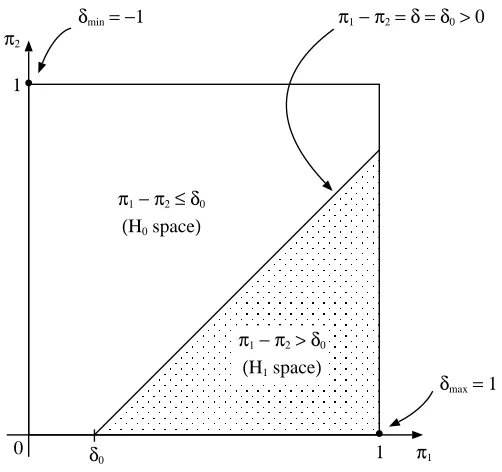
serve the role of _p(_θ|x) as found in (1.4.8). To construct _C_β(x) in (1.4.8), a (1−_β)

confidence region for (_π₁_{, π}₂)∈Θ₀ is generated by the cross product of two (1−_β)1/2

Clopper Pearson confidence intervals (Clopper and Pearson, 1934), one for _π₁ and

the other for_π₂. The details of constructing Clopper Pearson confidence intervals are

provided in the Appendix. Given a particular observation (_{X, Y}) = (_{x, y}), we will

use (_l₁_{, u}₁) and (_l₂_{, u}₂) to denote the Clopper Pearson confidence intervals for _π₁ and

π2 respectively. The (1−β) confidence region for (π1, π2)∈Θ0 is [l1, u1]×[l2, u2]∩H0

(28)

)

0 ₁ _π₁

δmax = 1

(H1space)

( )

l1 u1

l2

Figure 1.2: Shaded area is the (1−β) confidence region for (π₁, π₂) ∈ Θ₀. (l₁, u₁) and (l₂, u₂) denote the Clopper Pearson confidence intervals for π₁ and π₂ respectively.

In the next chapter, we examine the performance of the confidence region

p-value method versus that of the standard method under the framework of testing

for superiority and noninferiority by comparing rejection regions and corresponding

size plots. By inverting these exact tests, we derive exact confidence intervals for

the parameter of interest. In the following chapter, we examine the performance of

the two confidence interval methods through coverage probability and interval length

comparisons.

(29)

Comparison of Unconditional

Exact Tests for Testing the

Difference of Independent

Binomial Proportions

Our comparison of the unconditional exact tests will be discussed separately under

the context of testing for superiority and noninferiority. We begin our discussion with

superiority.

(30)

For clinical trials where a new treatment is compared to a standard control,

re-searchers are often interested in testing whether the treatment is significantly better

than, orsuperior to, the control. There are different definitions of null and alternative

hypotheses in establishing superiority. Some define the appropriate hypotheses to be:

H0 : π1 ≤π2

H1 : π1 > π2.

(2.1.1)

Others define the appropriate hypotheses to be:

H0 : π1 −π2 ≤δ0

H1 : π1 −π2 > δ0,

(2.1.2)

where _δ₀ _> 0 is a clinically significant value determined by researchers. In order to

differentiate between these two sets of hypotheses, some, such as Mart´ın Andr´es and

Herranz Tejedor (2002), refer to the hypotheses in (2.1.1) in the context ofsuperiority

and the hypotheses in (2.1.2) in the context of substantial-superiority. Figure 1.1

represents the hypothesis spaces specified by (2.1.1), and Figure 2.1 represents the

hypothesis spaces specified by (2.1.2). In this work, we will not make the distinction

between these two labels and will refer, in general, to hypotheses in the form of (2.1.2)

in the context of superiority.

(31)

0 ₁ _π₁

δmax = 1

(H0space)

π1 − π2 > δ0 (H1space)

δ0

Figure 2.1: Superiority hypothesis spaces as specified by (2.1.2).

2.1.2 Computation Study

In the context of hypothesis testing for superiority, we have examined the

perfor-mances of the competing exact methods under various settings of the sample sizes_n₁

and _n₂. Namely, we examined a total of nine sample size combinations of (_n₁_{, n}₂),

where_n₁ :_n₂ ∈ {1:1_,2:1_,3:1}and_n₁+_n₂ ∈ {20_,60_,100}. The hypotheses of interest,

H0 : δ ≤δ0 versus H1 :δ > δ0, were examined under δ0 ∈ {0.0,0.1,0.2, . . . ,0.9} and

at significance levels_α ∈ {0_.01_,0_.05_,0_.10}. We have included the _δ₀ = 0 case here so

that, combined with our noninferiority study to be discussed later, analyses based on

a complete range of _δ₀ values will be performed. Thus, our analyses in this section

will be based on both (2.1.1) and (2.1.2).

Since we will often refer to the tests based on _p_r and_p_u, let us denote the _α level

(32)

2.1.3 Examples of

_T

_p_r

Performance Relative to

_T

_p_u

Probability Plot Example: (_{x, y})∈ R_p_r, (_{x, y})6∈ R_p_u

Before discussing the complete results from our computation study, let us take a

close examination of a probability plot based on a particular sample point where the

pr method proves to be advantageous.

In Figure 2.2 we consider the probability plot for the sample point (_{x, y}) = (30_,16),

where (_n₁_{, n}₂) = (50_,50), _δ₀ = 0_.10, and _α = 0_.05. The unrestricted p-value

prob-ability plot is represented by the dash-dot line. Note that the graph is based upon

the entire nuisance parameter space (0_.1_,1). The p-value _p_u is defined as the

max-imum height of the plot, approximately 0.058, which clearly exceeds the horizontal

reference line of _α = 0_.05. Thus, (_{x, y}) = (30_,16) would not be included in the set

Rpu. Notice that the peaks of the pr graph, which appear near the extremes of the

nuisance parameter space, are the culprits responsible for keeping (30_,16) out ofR_p_u.

Much of the _p_u graph is well below the _α level. However, the conservative approach

of the unrestricted p-value method dictates that we consider the worst case scenario,

even when such a scenario is not well supported by the data.

(33)

respectively in Figure 2.2. This confidence interval is used as the restricted domain of

the dash-dot probability plot in determining _p_r. To be more specific, the p-value _p_r

is defined as the maximum of the restricted domain probability plot plus the penalty

term of _β = 0_.001. This modified probability plot is shown by the solid curve lying

above the dash-dot curve. Note that the restricted domain lies significantly away

from the endpoints of the entire nuisance parameter space. With the added penalty

term of_β, we see that the maximum of the solid curve is approximately 0.039. Thus,

(_{x, y}) = (30_,16) would be included in the setR_p_r.

Figure 2.2 is a good illustration of how conservative the_p_u method can be. Using

a restricted interval with high confidence of 99.9%, the data indicate the true value

of the nuisance parameter is closer to the center of the parameter space as opposed

to the ends where the sharp peaks of the probability plot exist.

(34)

0.2 0.4 0.6 0.8 1.0

0.035

0.040

0.045

0.050

Probability

Nuisance Parameter

L U

Figure 2.2: (x, y) ∈ R_p_r, (x, y) 6∈ R_p_u. Probability plot for testing H₀ : δ ≤ 0.10 at the

α= 5% level given (n₁, n₂) = (50,50) and observation (x, y) = (30,16). The dash-dot line is based onp_u, the solid line is based onp_r. The pointsLandUare, respectively, the lower and upper limits of π₁ based on the confidence region (β= 0.001) p-value approach.

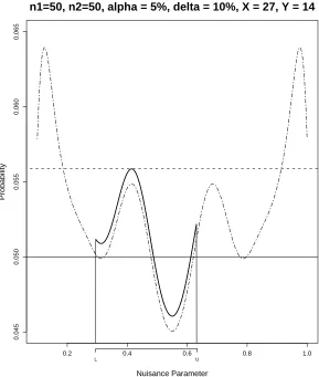
Probability Plot Example: (_{x, y})6∈ R_p_r, (_{x, y})6∈ R_p_u

Now, let us consider an example where the sample point is excluded from both

rejection regions. In Figure 2.3 we consider the probability plot for the sample point

(_{x, y}) = (27_,14). This is, again, from the analysis of the (_n₁_{, n}₂) = (50_,50),_δ₀ = 0_.10,

and _α= 0_.05 setting. The unrestricted p-value probability plot is represented by the

(35)

For this example the _p_r approach does not help in capturing (27,14) in R_p_r. We

calculated our 99.9% confidence region for the nuisance parameter to be (0.249,0.633).

Again, the lower and upper limits of this confidence interval are represented byLandU

respectively in Figure 2.3. The modified_p_rprobability plot is shown by the solid curve

lying above the dash-dot curve. With the added penalty term of _β = 0_.001, we see

that the maximum of the solid curve is approximately 0.056. Thus, (_{x, y}) = (27_,14)

is also excluded from the set R_p_r.

Although it is the case that the sample point was excluded from both rejection

regions, it is worth noting in this example that the _p_r p-value was less conservative

than the corresponding _p_u p-value. With this in mind, the _p_r method does offer an

advantage in that it yields stronger evidence against the null hypothesis of interest.

Later, when we discuss testing for noninferiority, we will illustrate an example showing

how the _p_r method can be disadvantageous.

(36)

0.2 0.4 0.6 0.8 1.0

0.045

0.050

0.055

Probability

Nuisance Parameter

L U

Figure 2.3: (x, y) 6∈ R_p_r, (x, y) 6∈ R_p_u. Probability plot for testing H₀ : δ ≤ 0.10 at the

α= 5% level given (n₁, n₂) = (50,50) and observation (x, y) = (27,14). The dash-dot line is based onp_u, the solid line is based onp_r. The pointsLandUare, respectively, the lower and upper limits of π₁ based on the confidence region (β= 0.001) p-value approach.

2.1.4 Results

Rejection region comparisons based upon all ten _δ₀ values are summarized in

Tables 2.1 through 2.10. In each of the tables, we use |R_p_r| and |R_p_u| to denote

the cardinalities of the rejection regions based on_p_r and _p_u respectively. |R_p_u\ R_p_r|

refers to the number of points of R_p_u not common toR_p_r. Analogously, |R_p_r \ R_p_u|

(37)

n1 :n2 = 1:1

For _n₁ :_n₂ = 1:1, the two rejections regions are often identical. This is especially

the case for (_n₁_{, n}₂) = (10_,10) and (30_,30). For higher values of _δ₀, the number of

sample points captured in either rejection region diminishes leaving little room for

the two sets to be very different. Thus, it is not surprising to see entries that are very

close to or equal to zero for |R_p_u\ R_p_r|and |R_p_r \ R_p_u|for larger _δ₀. This, of course,

will be a common phenomenon across all sample size ratios.

One important case worth noting is (_n₁_{, n}₂) = (50_,50). For _δ₀ = 0_.10 and 0_.20,

we see that R_p_u is contained in R_p_r at each significance level setting. That is, _T_p_r is

uniformly more powerful than _T_p_u.

In Table 2.2, we limited our focus on_n₁+_n₂ = 20, 60, and 100 and we discovered

the _p_r method yielded benefits for the largest sample size sum. We performed a

further analysis of other 1:1 ratios to gain a better understanding of the performance

of _T_p_r based upon popularly used balanced sample size cases. This information is

summarized in Table 2.11. Based on this table, we see that, in the case where _δ₀ =

0_.10,_T_p_r is found to be more powerful from as early as _n₁ =_n₂ = 40. With the seven

sample size settings found in (_n₁_{, n}₂) ∈ {(40_,40)_,(50_,50)_{, ...,}(100_,100)}, keeping in

mind the three levels of _α, this leads to a total of 21 possible analyses. Of these

(38)

nearly contains all ofR_p_u. Overall, we can see that the_p_r method performs very well,

in general, for 1:1 cases when_n₁+_n₂ ≥80. Later, we will investigate this further by

discussing an interesting feature of the size plot based on (_n₁_{, n}₂) = (100_,100).

n1 :n2 = 2:1

For _n₁ : _n₂ = 2:1, the performance of the _p_r based test improves. Note that, in

many cases,R_p_u is a proper subset ofR_p_r. For example, in Table 2.2 where_δ₀ = 0_.10,

Tpr is uniformly more powerful in virtually all cases for (n1, n2) = (40,20) and (66,34).

In the smallest sample size setting (_n₁_{, n}₂) = (13_,7), _T_p_r does not offer much of an

advantage. It is worth noting that, when _T_p_u is uniformly more powerful than that

of _T_p_r, the R_p_u rejection region typically contains only one or two more points than

those contained in R_p_r. In Table 2.3 where _δ₀ = 0_.20, _T_p_r is again uniformly more

powerful in virtually all cases for (_n₁_{, n}₂) = (40_,20) and (66_,34). Here, we see that

a mixed result appears in this table for (_n₁_{, n}₂) = (40_,20) and _α = 0_.01. Note that

|Rpu\ Rpr|= 2, whereas |Rpr \ Rpu|= 8. Thus, neither rejection region is a proper

subset of the other and hence the corresponding size plots would cross. An important

observation to note is that, when the rejection setR_p_u gains additional points beyond

that of R_p_r, this gain is small relative to the number of points the rejection set R_p_r

(39)

n1 :n2 = 3:1

For _n₁ :_n₂ = 3:1, the performance of _T_p_r continues to improve. _T_p_r is at least as

powerful as, and many times uniformly more powerful than,_T_p_u. We note again that,

as in the 2:1 case,_T_p_r does not offer any advantages for the smallest sample size setting.

When (_n₁_{, n}₂) = (45_,15) or (75_,25) the benefit of using _T_p_r is quite apparent. As

discovered in the 2:1 case, we find that_p_r is not uniformly more powerful for all cases.

As an example, consider Table 2.2 where _δ₀ = 0_.10. For (_n₁_{, n}₂) = (75_,25), except

for the case where _α = 5%, we see that mixed results appear. However, as in the

mixed result case discussed in the previous sample size ratio, we note that|R_p_u\ R_p_r|

is small relative to |R_p_r \ R_p_u|. For example, in the _α = 1% case, |R_p_u \ R_p_r| = 3,

whereas|R_p_r\ R_p_u|= 21. In general, this relationship is maintained in the remaining

tables as well. The summary for the 2:1 case is applicable once again: the gains of

the _p_r method outweigh the losses it incurs.

(40)

0.01 |R_pu| 17 261 833 14 217 703 9 172 556

|Rpr| 17 259 831 13 223 722 9 175 578

|Rpu\ Rpr| 0 2 4 1 0 1 0 0 0

|Rpr\ Rpu| 0 0 2 0 6 20 0 3 22

0.05 |R_pu| 29 322 967 24 271 843 19 228 689

|Rpr| 29 322 967 24 278 854 19 229 695

|Rpu\ Rpr| 0 0 0 0 0 0 0 0 1

|Rpr\ Rpu| 0 0 0 0 7 11 0 1 7

0.10 |R_pu| 32 345 1016 30 306 914 20 230 689

|Rpr| 32 351 1034 30 309 920 22 251 750

|Rpu\ Rpr| 0 0 0 0 0 0 0 0 0

|Rpr\ Rpu| 0 6 18 0 3 6 2 21 61

(41)

0.01 |R_pu| 12 193 619 10 138 514 4 96 410

|Rpr| 12 193 629 8 159 547 4 120 428

|Rpu\ Rpr| 0 0 0 2 0 0 0 0 3

|Rpr\ Rpu| 0 0 10 0 21 33 0 24 21

0.05 |R_pu| 19 247 718 16 216 659 10 147 519

|Rpr| 19 247 741 16 216 662 10 168 534

|Rpu\ Rpr| 0 0 0 0 0 0 0 0 0

|Rpr\ Rpu| 0 0 23 0 0 3 0 21 15

0.10 |R_pu| 25 277 801 21 231 698 19 200 587

|Rpr| 25 277 810 22 239 721 18 200 591

|Rpu\ Rpr| 0 0 0 0 0 0 1 0 1

|Rpr\ Rpu| 0 0 9 1 8 23 0 0 5

(42)

0.01 |R_pu| 8 134 452 7 107 369 4 82 298

|Rpr| 8 136 463 5 113 397 4 89 310

|Rpu\ Rpr| 0 0 0 2 2 0 0 0 0

|Rpr\ Rpu| 0 2 11 0 8 28 0 7 12

0.05 |R_pu| 14 179 556 13 158 486 6 115 396

|Rpr| 14 179 562 13 159 494 6 123 401

|Rpu\ Rpr| 0 0 0 0 0 0 0 0 0

|Rpr\ Rpu| 0 0 6 0 1 8 0 8 5

0.10 |R_pu| 19 206 611 16 179 530 12 151 428

|Rpr| 19 206 613 16 181 546 12 150 448

|Rpu\ Rpr| 0 0 0 0 0 0 0 1 0

|Rpr\ Rpu| 0 0 2 0 2 16 0 0 20

(43)

0.01 |R_pu| 5 97 318 4 77 264 2 53 213

|Rpr| 5 97 322 4 79 277 2 57 215

|Rpu\ Rpr| 0 0 0 0 0 0 0 0 2

|Rpr\ Rpu| 0 0 4 0 2 13 0 4 4

0.05 |R_pu| 10 132 412 9 114 347 5 76 279

|Rpr| 10 132 410 9 112 358 5 88 288

|Rpu\ Rpr| 0 0 2 0 2 0 0 0 0

|Rpr\ Rpu| 0 0 0 0 0 11 0 12 9

0.10 |R_pu| 14 154 455 11 127 394 9 105 328

|Rpr| 14 152 455 11 130 402 9 106 329

|Rpu\ Rpr| 0 2 0 0 0 0 0 0 0

|Rpr\ Rpu| 0 0 0 0 3 8 0 1 1

(44)

0.01 |R_pu| 3 63 220 1 51 189 0 36 132

|Rpr| 3 59 220 1 50 188 0 35 138

|Rpu\ Rpr| 0 4 0 0 1 1 0 2 0

|Rpr\ Rpu| 0 0 0 0 0 0 0 1 6

0.05 |R_pu| 6 90 282 5 71 250 3 61 199

|Rpr| 6 90 282 5 74 250 3 61 197

|Rpu\ Rpr| 0 0 0 0 0 0 0 0 2

|Rpr\ Rpu| 0 0 0 0 3 0 0 0 0

0.10 |R_pu| 8 107 318 8 93 278 6 74 223

|Rpr| 8 105 318 8 93 280 6 75 229

|Rpu\ Rpr| 0 2 0 0 0 0 0 0 0

|Rpr\ Rpu| 0 0 0 0 0 2 0 1 6

(45)

0.01 |R_pu| 1 38 138 1 29 109 0 19 84

|Rpr| 1 38 132 1 28 111 0 20 84

|Rpu\ Rpr| 0 0 6 0 1 0 0 0 0

|Rpr\ Rpu| 0 0 0 0 0 2 0 1 0

0.05 |R_pu| 3 57 179 2 45 155 2 33 116

|Rpr| 3 55 179 2 45 157 2 36 124

|Rpu\ Rpr| 0 2 0 0 0 0 0 0 0

|Rpr\ Rpu| 0 0 0 0 0 2 0 3 8

0.10 |R_pu| 6 66 202 5 59 185 3 47 144

|Rpr| 6 66 208 5 59 186 3 47 149

|Rpu\ Rpr| 0 0 0 0 0 0 0 0 0

|Rpr\ Rpu| 0 0 6 0 0 1 0 0 5

(46)

0.01 |R_pu| 0 19 72 0 13 60 0 10 41

|Rpr| 0 19 72 0 13 61 0 8 40

|Rpu\ Rpr| 0 0 0 0 0 0 0 2 2

|Rpr\ Rpu| 0 0 0 0 0 1 0 0 1

0.05 |R_pu| 1 32 105 1 23 93 0 21 71

|Rpr| 1 32 105 1 25 93 0 20 71

|Rpu\ Rpr| 0 0 0 0 0 0 0 1 0

|Rpr\ Rpu| 0 0 0 0 2 0 0 0 0

0.10 |R_pu| 3 40 124 2 33 111 2 27 85

|Rpr| 3 40 124 2 33 111 2 27 88

|Rpu\ Rpr| 0 0 0 0 0 0 0 0 0

|Rpr\ Rpu| 0 0 0 0 0 0 0 0 3

(47)

0.01 |R_pu| 0 8 34 0 5 23 0 3 16

|Rpr| 0 6 32 0 5 24 0 3 16

|Rpu\ Rpr| 0 2 2 0 0 0 0 0 0

|Rpr\ Rpu| 0 0 0 0 0 1 0 0 0

0.05 |R_pu| 1 15 53 0 13 45 0 9 34

|Rpr| 1 15 53 0 13 45 0 9 34

|Rpu\ Rpr| 0 0 0 0 0 0 0 0 0

|Rpr\ Rpu| 0 0 0 0 0 0 0 0 0

0.10 |R_pu| 1 21 66 1 16 58 0 12 44

|Rpr| 1 21 65 1 16 58 0 13 44

|Rpu\ Rpr| 0 0 1 0 0 0 0 0 0

|Rpr\ Rpu| 0 0 0 0 0 0 0 1 0

(48)

0.01 |R_pu| 0 1 10 0 0 7 0 0 4

|Rpr| 0 1 10 0 0 7 0 0 4

|Rpu\ Rpr| 0 0 0 0 0 0 0 0 0

|Rpr\ Rpu| 0 0 0 0 0 0 0 0 0

0.05 |R_pu| 0 5 19 0 3 16 0 2 11

|Rpr| 0 5 17 0 3 16 0 2 11

|Rpu\ Rpr| 0 0 2 0 0 0 0 0 0

|Rpr\ Rpu| 0 0 0 0 0 0 0 0 0

0.10 |R_pu| 0 6 21 0 6 22 0 4 16

|Rpr| 0 6 21 0 6 22 0 4 16

|Rpu\ Rpr| 0 0 0 0 0 0 0 0 0

|Rpr\ Rpu| 0 0 0 0 0 0 0 0 0

(49)

0.01 |R_pu| 0 0 1 0 0 0 0 0 0

|Rpr| 0 0 1 0 0 0 0 0 0

|Rpu\ Rpr| 0 0 0 0 0 0 0 0 0

|Rpr\ Rpu| 0 0 0 0 0 0 0 0 0

0.05 |R_pu| 0 1 3 0 0 2 0 0 0

|Rpr| 0 1 3 0 0 2 0 0 0

|Rpu\ Rpr| 0 0 0 0 0 0 0 0 0

|Rpr\ Rpu| 0 0 0 0 0 0 0 0 0

0.10 |R_pu| 0 1 3 0 0 3 0 0 2

|Rpr| 0 1 3 0 0 3 0 0 2

|Rpu\ Rpr| 0 0 0 0 0 0 0 0 0

|Rpr\ Rpu| 0 0 0 0 0 0 0 0 0

(50)

α (10) (20) (30) (40) (50) (60) (70) (80) (90) (100)

0.01 |R_pu| 12 74 193 383 619 935 1284 1722 2295 2794

|Rpr| 12 74 193 379 629 947 1333 1789 2321 2915

|Rpu\ Rpr| 0 0 0 4 0 0 2 0 2 0

|Rpr \ Rpu| 0 0 0 0 10 12 51 67 28 121

0.05 |R_pu| 19 99 247 457 718 1099 1541 1981 2591 3265

|Rpr| 19 99 247 459 741 1105 1539 2033 2613 3271

|Rpu\ Rpr| 0 0 0 0 0 0 2 0 0 0

|Rpr \ Rpu| 0 0 0 2 23 6 0 52 22 6

0.10 |R_pu| 25 113 277 481 801 1180 1640 2108 2736 3441

|Rpr| 25 113 277 501 810 1186 1644 2166 2774 3447

|Rpu\ Rpr| 0 0 0 0 0 0 0 0 0 0

|Rpr \ Rpu| 0 0 0 20 9 6 4 58 38 6

(51)

correspond to the information found in Table 2.2. In the interest of space, we provide

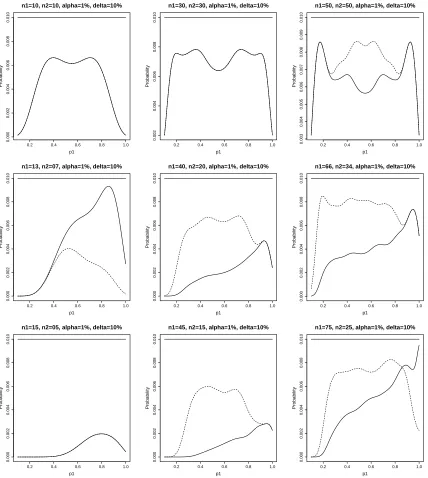
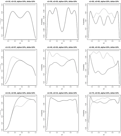
size plots only for _δ₀ = 0_.10, although the figures are sufficient to illustrate the

behavior of _T_p_r relative to _T_p_u. In each figure, the plots are arranged in an array of

three rows and three columns. The rows, from top to bottom, correspond to sample

size ratios of 1:1, 2:1, and 3:1 respectively. The columns, from left to right, correspond

to _n₁ +_n₂ = 20, 60, and 100 respectively. For each plot, the solid line refers to_T_p_u,

the dotted line refers to _T_p_r.

From the plots we again note that _T_p_r is not as powerful when _n₁+_n₂ = 20 (first

column). However, for the second and third columns, we find that, in general, _T_p_r is

at least as powerful as _T_p_u. The mixed results we alluded to earlier is illustrated in

Figures 2.4 and 2.6 for (_n₁_{, n}₂) = (75_,25) by the crossing of the two graphs.

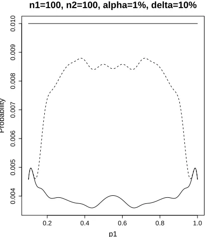
Referring back to our in-depth investigation of the 1:1 sample size cases

summa-rized in Table 2.11, a size plot based upon (_n₁_{, n}₂) = (100_,100) illustrates how

con-servative_T_p_u can be. This plot is given in Figure 2.7. Notice that the solid line based

upon_p_u achieves a maximum height of onlyhalf the value of the level of significance.

To investigate this further, we determined that the rejection region to construct the

size plot for _T_p_u in Figure 2.7 and considered what would occur to the probability

plot when the next extreme point from the sample space was included. This

(52)

corresponding to this set is represented by the broken line in Figure 2.8. As shown

in the figure, the updated set causes the probability plot to jump significantly to a

height just above the level of significance (0_.010007_>0_.01). Because of this fact, the

Tpu size is forced unusually below the level of significance making it very conservative.

(53)

0.2 0.4 0.6 0.8 1.0

0.000

0.002

p1

0.2 0.4 0.6 0.8 1.0

0.002

0.004

p1

0.2 0.4 0.6 0.8 1.0

0.003

0.004

p1

0.2 0.4 0.6 0.8 1.0

0.000 0.002 0.004 0.006 0.008 0.010

n1=13, n2=07, alpha=1%, delta=10%

p1 P ro b a bili ty

0.2 0.4 0.6 0.8 1.0

0.000 0.002 0.004 0.006 0.008 0.010

n1=40, n2=20, alpha=1%, delta=10%

p1 P ro b a bili ty

0.2 0.4 0.6 0.8 1.0

0.000 0.002 0.004 0.006 0.008 0.010

n1=66, n2=34, alpha=1%, delta=10%

p1 P ro b a bili ty

0.2 0.4 0.6 0.8 1.0

0.000 0.002 0.004 0.006 0.008 0.010

n1=15, n2=05, alpha=1%, delta=10%

p1 P ro b a bili ty

0.2 0.4 0.6 0.8 1.0

0.000 0.002 0.004 0.006 0.008 0.010

n1=45, n2=15, alpha=1%, delta=10%

p1 P ro b a bili ty

0.2 0.4 0.6 0.8 1.0

0.000 0.002 0.004 0.006 0.008 0.010

n1=75, n2=25, alpha=1%, delta=10%

p1 P ro b a bili ty

Figure 2.4: Size plots for testingH₀:δ≤0.10 at theα= 1% level. The solid line is based onT_p_u, the dotted line is based onT_p_r. The rows, from top to bottom, correspond to sample size ratios of 1:1, 2:1, and 3:1 respectively. The columns, from left to right, correspond to

n1+n2= 20, 60, and 100 respectively.