Web pre-fetching schemes using Machine Learning for Mobile Cloud Computing

(1)

Int. J. Advance Soft Compu. Appl, Vol. 9, No. 2, July 2017 ISSN 2074-8523

Web Pre-fetching Schemes using Machine

Learning for Mobile Cloud Computing

Nur Syahela Hussien and Sarina Sulaiman

UTM Big Data Centre,Universiti Teknologi Malaysia, 81310 Skudai Johor. e-mail: [email protected], [email protected]

Abstract

Pre-fetching is one of the technologies used in reducing latency

on network traffic on the Internet. We propose this technology to utilise Mobile Cloud Computing (MCC) environment to handle latency issues in context of data management. However, overaggressive use of the pre-fetching technique causes overhead and slows down the system performance since pre-fetching the wrong objects data wastes the storage capacity of a mobile device. Many studies have been using Machine Learning (ML) to solve such issues. However, in MCC environment, the pre-fetching using ML is not widely used. Therefore, this research aims to implement ML techniques to classify the web objects that require decision rules. These decision rules are generated using few ML algorithms such as J48, Random Tree (RT), Naive Bayes (NB) and Rough Set (RS).These rules represent the characteristics of the input data accordingly. The experimental results reveal that J48 performs well in classifying the web objects for all three different datasets with testing accuracy of 95.49%, 98.28% and 97.9% for the UTM blog data, IRCache, and Proxy Cloud Computing (CC) datasets respectively. It shows that J48 algorithm is capable to handle better cloud data management with good recommendation to users with or without the cloud storage.

Keywords: web pre-fetching, mobile cloud computing, machine learning techniques

1 Introduction

(2)

155 Web Pre-fetching Schemes using Machine

mobile devices. Users can have unlimited online access and may access unlimited space for data storage [1]–[4]. However, the data management issue is observed as one of the issues in MCC [5]–[7]. Sometimes users have a problem to save their data when the storage is already full and they need to manually find out if there is still available space. The current CC service normally has a limitation in storage capacity. For example, the Dropbox application only provides 2GB free storage and 5GB for a Skydive and Sugarsync. In addition, a user needs to pay per use [8][8], [9]. Thus, some users use several types of CC service to support their data storage but they encounter with data management problems in handling their data. Besides, there are too long for loading time to access their data when there are too many Cloud Storage Services (CSS) at the same time. They need to find the CSS data they put their data on. Due to this situation, we suggested improvement by applying ML technique to maintain the quality of the service needed. One of the best techniques to enhance the system performance is web caching and pre-fetching by keeping the web objects, which are expected for future visit closer to the clients.

Web caching can work alone or integrate with web pre-fetching. The web caching and pre-fetching can synchronise between each other because web-caching uses the temporal area to forecast revisiting requested objects, while web pre-fetching predicts web objects that might be requested in the near future. Then, the predicted objects are fetched from the origin server, which are stored in a cache. Thus, web pre-fetching helps to increase the cache hits and reduce the user-perceived latency [7], [10], [11]. Thus, this data is available immediately upon request, which eliminates the loading time perceived by the user.

(3)

Hussien. N.S. et al. 156

However, overaggressive fetching affects the performance because pre-fetching overhead occurs if the pre-pre-fetching data is unused. Hence, it needs the best pre-fetch algorithm to optimise the performance. Therefore, this paper proposed a new work to determine and analyse the ML techniques that can be applied in optimising the pre-fetching performance[16], [17]. There is no single technique that is better than the others in solving all problems. This is discussed by several authors. The most noteworthy is probably by Wolpert [18] in his research on the lack of a priori distinctions between learning algorithms. Therefore, the way is by making a test of multiple algorithms and parameter settings. In this study, we investigate the performance of J48, RT, NB and RS to test their ability to discover patterns and make accurate pre-fetching predictions. Then, reveal the technique with the highest accuracy, which can be applied in generating the rules for pre-fetching of future objects being requested. Thus, an ML technique is required to enhance the pre-fetching techniques because ML can learn and predict the right data requested by users. If only pre-fetching is used, it may pre-fetch the wrong data that will cause overhead and use a lot of memory that store useless data. This is important to make sure the techniques have efficient use of the limited amount of memory available in mobile devices. Before proposes the scheme, the previous pre-fetching schemes have been study on the next section 2. There are some pre-fetching scheme have been proposed before this, however there are applied in different field study area. The schemes have their own characteristic that suitable with their proposed work. The scheme show and explain on how the pre-fetching apply in their research work to reduce the latency issues based on their field area.

The rest of the paper is organised as follows: Section 3 elaborates on the propose intelligent mobile web pre-fetching scheme including the data collection, data pre-processing, ML techniques and performance evaluation on proposed ML techniques. Section 4 discuss on the results experiment. Finally, Section 5concludes the article and discusses future work for our research.

2 Previous Pre-fetching Schemes

(4)

operations in directing what data should be fetched on storage servers in advance. At last, the pre-fetched data could be pushed to the relevant client machine from the storage server. The results reveal that the initiative pre-fetching technique can effectively and practically forecast future disk operations to guide data pre-fetching for different workloads with acceptable overhead.

The scheme of initiative data pre-fetching is a novel idea presented in this paper, and the architecture of this scheme is demonstrated in Figure1 while it handles read requests (the assumed synopsis of a read operation is read (int files, size t size, off t off)). In the figure, the storage server can predict the future read operation by analysing the history of disk I/Os, so that it can directly issue a physical read request to fetch data in advance. The most attractive idea in the figure is that the pre-fetched data will be forwarded to the relevant client file system proactively, but the client file system is not involved in both prediction and pre-fetching procedures. Finally, the client file system can respond to the hit read request sent by the application with the buffered data. As a result, the read latency on the application side can be reduced significantly. Furthermore, the client machine, which might have limited computing power and energy supply can focus on its own work rather than predicting related tasks.

Fig 1: Architecture for the scheme of initiative data pre-fetching by Liao et al. [19].

(5)

in Fig.2, when user A gets an interesting RSS update of a music video (MV) from his/her RSS subscription, pre-fetching level “mid” should be chosen; however, because A is connected by 3G, pre-fetching will be downgraded to “low.” User B gets direct recommendation of the RSS from A, and thus, B’s subVB will pre-fetch the video at the level of “all.” However, B is also connected by 3G; hence, only “mid” level pre-fetching is triggered. User C sees B’s rating activity of the RSS feed while C is connected by Wi-Fi, and thus, C’s subVB will push a small part of the content to the device at “low” level.

Fig 2: Illustration of social sharing by Wang and Chen [20]

Moreover, Sharma and Dubey [21] provided a semantic-based pre-fetching scheme for the web browsers to overcome the limitations of existing systems as in Fig. 3.

Fig 3: Semantic based web pre-fetching scheme by Sharma and Dubey [21]. Lexical Analyser

Browser

Server User

Anchor

Find Anchor Text

Convert Anchor Text into Tokens

Compute Probability of Tokens

SPRINT (Decision

Tree) Pre-fetcher

Patterns

Pre-fetch List

Storage Unit Optimal Page Replacement Algorithm

(6)

Semantic-based pre-fetching uses anchor text as a base for finding out patterns. Anchor text is present in the hyperlinks of web page. With the help of anchor text, ranking of web page that will be received by search engine can also be determined. This scheme applies Decision Tree Induction in computing the probability of the anchor text and finding out patterns to be pre-fetched.

A novel Cluster and Pre-fetch (CPF) approach was proposed by Raju and Sudhamani [22]. Experimental results showed that the CPF approach effectively reduced the user perceived latency without wasting the network resources with high prediction accuracy. Most pre-fetching techniques predict the Web page requests for individual user. These techniques can easily overload the network when there are large numbers of users. To overcome this, Cluster and Pre-fetch (CPF) approaches were proposed in this paper. These approaches used the ART1 NN clustering algorithm to cluster the Web users. The prototype vector of each cluster gave a generalised representation of the Web pages that were most frequently requested by all the members of that cluster. Whenever a host connected to the server or a proxy, the proposed pre-fetching strategy returned the Web pages for the cluster to which the host belonged to. An advantage of the CPF approach is that better network resource utilisation by pre-fetching the Web pages for a user community rather than a single user, thereby improving the Web browsing time of user. The architecture of the CPF model is as shown in Fig. 4. The feature extractor module extracts each client’s feature vector.

Fig 4: Architecture of CPF Approach by Raju and Sudhamani [22].

(7)

a community of users instead of a single user. Though the CPF approach results in substantial increase of network traffic, it effectively reduces the user perceived latency.

Nevertheless there have been a lot of studies carried out in pre-fetching schemes, its usage in reducing latency in different field of study with different algorithms applied on their work. Many studies have been done using Machine Learning (ML) to solve such issues. Nevertheless, the pre-fetching using ML is not widely used in MCC environment. Therefore, this paper proposed a mobile web pre-fetching scheme that is explained in the next section to handle latency issues in contact of data management problem in Mobile Cloud Computing (MCC).

3 Proposed Intelligent Mobile Web Pre-fetching

Scheme

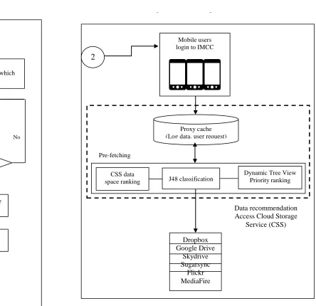
In this paper the proposed scheme aimed to enable multiple Cloud Storage Services (CSS) being accessed by mobile users at anytime and everywhere. Users can access their data faster by using IMCC because it predicts the data requested by future users based on ML technique. Besides, IMCC can make recommendation to store the data on CSS based on their availability. Fig. 5 shows the detailed flow of the proposed IMCC scheme. Based on the scheme, the data was extracted from three types of log data including the UTM blog, IRCache and Proxy CC. Then, the data was pre-processed by removal of irrelevant information from the present data set. Pre-processing is important before applying classification on the extracted data. The data was analysed based on four ML including the DT, RT, NB and RS.

(8)

Fig 5:The propose IMCC Scheme Yes

No Extracted data

Pre-fetching

Data recommendation Access Cloud Storage

Service (CSS)

Web log Data (UTM blog, IRCache, Proxy CC)

Identify the ML technique with the highest accuracy

of prediction?

Yes

Data Pre-processing

Data cleaned by filtering out all the log entries which have status code other than ‘200’

Extracted data

Select the ML technique that produces the highest accuracy (J48)

1

2

Analyse data using ML techniques such as the J48, RT, NB and RS

Mobile Cloud Computing Environment Rules Generation (Based on J48 algorithm)

Mobile users login to IMCC

J48 classification

Prediction of usage pattern

CSS data space ranking

Dynamic Tree View Priority ranking Proxy cache

(9)

The result came out in tree-view list by rank showing the highest probability data to be accessed by users in future. Besides, it provides the ability to make recommendation to user on CSS data space ranking. Consequently, users easily store their data on CSS, which is still available. Therefore, IMCC provides a convenience in handling user data management when using the MCC. Users access the data faster compared with traditional MCC. There are some materials involved in handling analysis including from the data sources, the software and also the hardware. The next section elaborates on material involved in this paper.

3.1 Data Collections

In this study, three log datasets were used including IRCache, UTM blog data and proxy CC dataset. The first data from IRCache was collected from a proxy server installation ftp://ircache.net. IRCache is a NLANR (National Laboratory of Applied Network Research) project that encourages web caching and provides data for researchers. In this study, 10591files were used for IRCache log data. IRCache regularly makes traces available to academic researchers. Besides, IRCache data is often used by other researchers in their research study [23], [24].

The second data was obtained from the UTM blog data consisting of 9103 requests for data transfer. The data was recorded on 13 January 2013, accessed by different client addresses. In addition, the third dataset used in this study was proxy CC dataset. Proxy CC was obtained by tracing the log data using Squid [25]–[29]. The sample of squid space area is as shown inFigure6. Moreover, Squid was used with some setup being done on the browser to collect the log data based on CC log data. The attributes were the same as another two datasets and contained1017 request data. This study uses this tree datasets because the datasets have similar attribute with the real work, hence it is easy to study and learn the pattern of datasets. Then, the results can be applied on real work. Normally there are various fields in log format:

• Time stamp of the request

• Time required in processing the request in millisecond • IP address of the machine requesting the object

• Cache Hit/Miss and Response Code • Requested item size in bytes

• Type of method used

• Requested object name/URL

• Information if the request is redirected to another server • Content type

An example of a line from a condensed log is:

(10)

Fig 6: Collecting data set using Squid

In order to run the experiment in this research, some hardware and software requirements were needed. The hardware requirements for this research were a personal computer with at least 2.0GHz, 2GB of memory and 500GB hard drive to be used in testing data. The software requirements for data analysis were WEKA and ROSETTA. Other data pre-processing software included the Microsoft excel and proxy log explorer.

Following the selection of the most appropriate input data, these data should undergo the pre-processed stage. Data pre-processing involved manipulating input data into a suitable form by scaling the data accordingly. Scaling of the data is important and essential, especially when the data is in different ranges. All collected data needed to be pre-processed as it was the key component to classify the object to be fetched. The next section explains in more detail the data pre-processing for this research work.

3.2 Data Pre-processing

(11)

Data cleaning is a process where irrelevant records are removed. The main aim of web usage mining is to fetch the traversal pattern; the following kinds of records are unnecessary and should be removed by using proxy explorer tool, Microsoft excel and WEKA tool.

a. The records having filenames suffixes of GIF, JPEG and CSS, which can be found in field of record.

b. The status fields of every record in the web log are examined, and all log entries, which have status code other than ‘200’ are filtered out. This is to ensure only the requests that fulfill the requirements are analysed to make further rules [25]–[32]

c. Entries with request methods except GET and POST

d. Remove uncatchable requests from the web proxy log file, requests that contain queries. Typically query requests contain the character “?” using Microsoft Excel.

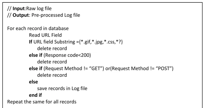
The major steps in the removal of irrelevant records from the data objects are presented in the form of algorithm in Figure7.

Fig 7: Algorithm for removing irrelevant records ii. User and Session Identification [31]:

The task in this step is to identify different user session from access log. A Referrer-based method is used to identify sessions. The different IP addresses distinguish different users.

// Input:Raw log file

// Output: Pre-processed Log file

For each record in database Read URL Field

If URL field Substring ={*.gif,*.jpg,*.css,*?}

delete record

else if (Response code<200)

delete record

else if (Request Method != “GET”) or(Request Method != “POST”)

delete record

else

save records in Log file

end if

(12)

iii. Path Completion:

Path Completion needs the complete user access path. The incomplete access path of every user session is recognised based on user session identification. If in the beginning of user session, Referrer as well URL has data value, delete value of Referrer by adding ‘_’. Web log pre-processing helps in removal of unwanted click-streams from the log file and reduces the size of original file by 40-50% [33].

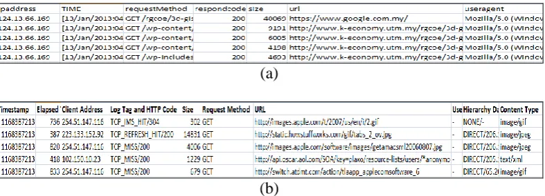
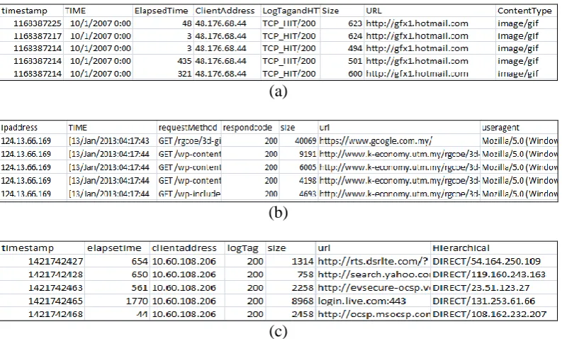
Fig.8 shows the actual data before data pre-processing and Figure9 depicts the pre-process data. Each line of a condensed log in log dataset corresponds to a single URL requested by the user. Table 1 gives the details of data before pre-processing and after pre-pre-processing. The individual access file was pre-processed carefully; the relevant details were retained as a training data set. The original size of the access data would be reduced remarkably after pre-processing. From that pre-processed data, total number of request, size of data source, number of unique user and number of frequent pages were identified and the samples are given in Table 1.

At this stage, three attributes were proposed based on the attributes that are widely used by the researchers in the area of web performance analysis [34], [35]. The attributes used in this study are:

i. Time: Time is the counter that observes the time takes to receive a data ii. Object Size: The size is in bytes

iii. Numbers of Hit: The number of hits per data

Each attribute must be multiplied with defined Priority Value (PV) to get the total sum of the attributes for target output generation of the network. The general formulation for expected target which is formulated in this study is shown as:

Expected target =

(size ∗ 0.266667) + (hit ∗ 0.200000) + (retrieval time ∗ 0.066667) (1)

(a)

(13)

(c)

Fig 8: Examples of data from UTM blog and IRCache and Proxy CC data: (a) UTM blog (b) IRCache (c) Proxy CC

(a)

(b)

(c)

(14)

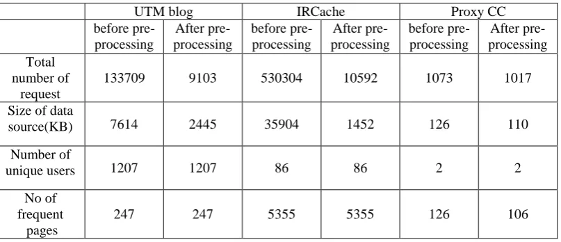
Table 1: Details of dataset before pre-processing and after pre-processing

UTM blog IRCache Proxy CC

before pre-processing

After pre-processing

After pre-processing Total

number of request

133709 9103 530304 10592 1073 1017

Size of data

source(KB) 7614 2445 35904 1452 126 110

Number of

unique users 1207 1207 86 86 2 2

No of frequent

pages

247 247 5355 5355 126 106

The summing up determines the expected target for current data. Commonly it is compared to a threshold number, and this threshold values are dynamic. A new threshold calculation is proposed based on the Latency ratio on singular Hit rate data [36]. The proposed threshold in this study could be written as an average of the maximum and the minimum of the related attributes multiply with the Priority Value. Mathematically, this can be represented as:

Threshold = ((sizemax+ sizemin/2) * 0.266667) + ((hitmax+ hitmin/2) * 0.200000) + ((timemax+ timemin/2) * 0.066667)

(2)

The threshold was calculated and updated for every epoch of the training. If the expected target was smaller than the threshold, then the expected target was 0, or else it became 1 if the expected target was equal or greater than that of the threshold shown below:

Expected Network Output = (3)

(15)

Normalised data, X =

(4)

On the other hand, the KNIME can also be used for the missing value replacement and the normalising procedure as shown in Figure 11. Using KNIME makes it easier for the user to normalise each datasets faster and more systematically.

(a) UTM blog (b) IRCache (c) Proxy CC

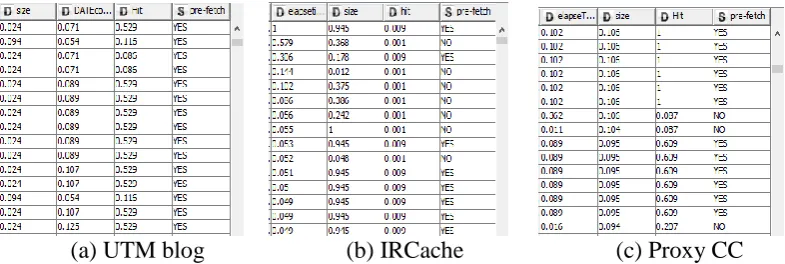
Fig 10:Examples of Normalised UTM blog and IRCache and Proxy CC data (a) UTM blog (b) IRCache (c) Proxy CC

Fig 11: KNIME environment for normalisation dataset

(16)

3.3 Machine Learning Techniques

The process flow in identifying the most effective technique for this research was by collecting data from the web log data. In this study, three datasets such as the UTM blog data, IRCache data and proxy CC, from which the features are extracted, were studied. All those three datasets were chosen because the log data field features are similar with the proposed work which is cloud computing data source. This paper also tested on cloud computing data itself, which is the Proxy CC. The data was cleaned by filtering out data with response code, 200. The 200 status code is the most common return that simply means the request was received and understood and is being processed [37]. Then, the DT, which are J48 and RT were used in the analysis by comparing them with another two algorithms, NB and RS. The analysis used the WEKA and ROSETTA tools to analyse the ML technique that provides high accuracy in prediction. About 70% of each dataset was used for training and the remaining was for the testing purposes. The performance of trend prediction systems was evaluated using the cross validation method. In cross-validation, a user needed to decide on a fixed number of folds or partitions of the data to find the best value. The data was randomly divided into 10 parts in which the class was represented in approximately the same proportions as in the full dataset [38]. The overall process is shown in pseudo code in Figure12.

Fig 12: Pseudo code for the proposed work on analysing data A.J48

A simple C4.5 decision trees for prediction of the DT the J48 classifier was used in this research. J48 is an open source java implementation of the C4.5 decision tree algorithm in the WEKA data mining tool that creates a binary tree. The DT approach is most useful in predicting problem [39]–[41]. Using this technique, a tree was constructed to model the prediction process. Figure 13 depicts the J48 algorithm as studied by Kumar and Reddy in [39]. While building a tree, J48 ignored the missing values. For example, the value of the item could be predicted based on what was known about the attribute values for the other records. The basic idea was to divide the data into range based on the attribute values for the

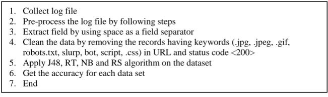
1. Collect log file

2. Pre-process the log file by following steps 3. Extract field by using space as a field separator

4. Clean the data by removing the records having keywords (.jpg, .jpeg, .gif, robots.txt, slurp, bot, script, .css) in URL and status code <200>

5. Apply J48, RT, NB and RS algorithm on the dataset 6. Get the accuracy for each data set

(17)

item found in the training sample. J48 allowed classification via either decision trees or rules generated from them [40].

J48 used the concept of information entropy. The training data was a set S = s1, s2, ... of already classified samples. Each sample si consisted of a p-dimensional vector (x1, i, x2, i,..., xp, i), where xj represented attributes or features of the sample, as well as the class in which si fell [39], [42]. At each node of the tree, J48 chose the attribute of the data that most effectively splits its set of samples into subsets enriched in one class or the other. The splitting criterion was the normalized information gain. The attribute with the highest normalised information gain was chosen to make the decision. The J48 algorithm then recurred on the smaller sub-lists.

Fig 13: J48 algorithm by Kumar and Reddy in [39]. B. Random Tree

Random Tree reminds the basic algorithm to build a decision tree using a portion of the data for the training dataset, and at each stage selects the feature and cut value that maximises the information gain. The earliest talk about RT was initiated by [43]. RT was built in two stages; the first was built independently of the training data, where a feature and cut value was randomly selected. Sometimes the result structure was called a tree skeleton. It repeated until the tree achieved the specified depth [44]. Regularly, there was a requirement that at each stage a new feature was selected. Secondly, the data training was used to specify the appropriate classifications or values. In general, multiple tree skeletons were computed and scoring for example prediction was done by combining the different trees into an ensemble as usual.

INPUT:

D //Training data OUTPUT T //Decision tree DTBUILD (*D) {

T=φ;

T= Creates root node and label with splitting attribute;

T= Adds arc to root node for each split predicate and label; For each arc do

D= Database created by applying splitting predicate to D; If stopping point reached this path,

then

T’= creates leaf node and label with appropriate class; }

(18)

Figure 14 is a simple summary of the training process of the random decision tree algorithm. The algorithm consists of two steps. The first step (BuildTreeStructure) generates the structure of each random tree. This is referred to as the skeleton since the leaves do not contain class distribution statistics. Building the skeleton does not require any training data, but instead only information about the features. In the second step called UpdateStatistics, the data training is used to compute class statistics for the leaf nodes.

Fig 14:Random Tree algorithm by Gao et al. in [44] C. Naïve Bayes

Naïve Bayes (NB) works very well on some domains, but poorly on others. NB is a straightforward and commonly used method for supervised learning. It provides a flexible way in dealing with any number of attributes or classes, and is based on probability theory. It is one of the fastest learning algorithms that examine all its training input. It has been established to execute surprisingly well in a very large range of problems despite the simplistic nature of the model [39]–[41], [45]. This technique is more useful when the dimensionality of input is enormous. It uses prior events to predict future events. Presuming an underlying probabilistic model allows us to capture uncertainty about the model in a principled way by determining probabilities of the outcomes. It can solve diagnostic and predictive problems. Additionally, a little amount of terrible data, or “noise,” does not affect the data analysis results.

NB is based on Bayes’ theorem and the theorem of total probability. The probability that a document d with vector x = < x1,...,xn> belongs to hypothesis h as follows [40]:

Train (S,X,N)

Data : training set S = {(x1,t1),...,(xn,tn)}, set of features X = {F1,...,Fk}.

F is a feature descriptor.

N is the number of random decision trees.

Result : N random trees {T1,...,TN}

begin

fori∈{1,...,N} do

BuildTreeStructure (Ti,X);

end

for(x,t) ∈S do

fori∈{1,..., N} do

UpdateStatistics(Ti,(x,t));

(19)

= (5)

Based on equation 5, P(h1|xi) is posterior probability, while P(h1) is the prior probability associated with hypothesis h1.

For m different hypotheses, they form equation 6,

(6)

Thus, equation 2 can be simplified as shown in equation 7,

(7)

If the web logs dataset contain many attributes, it will result in maximum computation time which can be reduced using the following equation P (Q | ) ≡ λ P( | ).

D. Rough Set

Data mining techniques are useful to solve analytical tasks in qualitative problems such as clustering, association, classification, dimension reduction, and forecasting. Among several data mining techniques, the RS is one of the excellent tools for classification analysis. RS, originally introduced by Pawlak in [46], is a valuable mathematical tool in dealing with imprecise or vague concepts.

(20)

concept. The lower approximation Y and the upper approximation Y of Y were defined as equations 8 and 9 [47]:

Y = {e ∈E | e ∈Ωi and Xi⊆Y} (8)

Ȳ = {e ∈E | e ∈Ωi and Xi ∩Y = ø} (9) Lower approximation is the intersection of all those elementary sets that are contained by Y, and upper approximation is the union of elementary sets that are contained by Y. Inductive Learning is a well-known area in artificial intelligence. It is used to form the information of human experts by using a carefully selected sample of expert decisions and inferring decision rules automatically, independent of the subject of interest.

In the proposed work, mathematical RS was applied to calculate the accuracy of classification. The method worked as follows.

a) Firstly, calculate number of items pre-set in the dataset. b) Next, do cross validation

It is sometimes called rotation estimation. It is a technique to assess how the results of a statistical analysis would generalise to an independent data set. According to Tiwari and Pandit in [49] cross validation expresses as a method to predict the fit of a model to a hypothetical validation set when an explicit validation set is not available.

(21)

Figure 15:JohnsonReducerand BatchClassifier algorithms for reducts searching and rules production by Hvidsten in [50].

3.4 Performance Evaluation

Performance evaluation was supported by results given using WEKA and ROSETTA. There are some parameter setting on WEKA and ROSETTA. When using WEKA it must be ensured that the output and input data selected is of the right, normally used file format such as ARFF or CSV. Then, the experiment type of datasets should be set as classification and divided into 70% for training and 30% for testing of the datasets. The number of repetition should be set with 10 by iteration and controlled with algorithm first, followed by the setting of the algorithms for data training and testing.

In order to set the parameter for ROSETTA, a simple analysis that induces a rules model on one part of the data (training set) should be done. This model should be used to classify the objects in the remaining data (test set) by set split factor with 0.7 for training and the remaining for testing RNG seed with 1. The Reduce and Johnson’s algorithm should be applied because the algorithm is very fast as it uses a greedy search to find one reduction. It should be set as Object related and it must be ensured that Approximate solutions is turned off under Advanced parameters. Then, the rules that classify the datasets must be set. Number of cross validation iterations is set with 10, which is the number of folds.

The performance evaluation is based on classifier evaluation metrics. Tables 2, 3 and 4 reveal the comparison of performance for J48, RT and NB using WEKA, then RS by using ROSETTA for three datasets. Mean and standard deviation were used as a statistical validation to verify the performance of those proposed

JohnsonReducer

{DISCERNIBILITY=Object; MODULO.DECISION=T; BRT=F; SELECTION=All; IDG=F; PRECOMPUTE=F; APPROXIMATE=F}

BatchClassifier

{CLASSIFIER=StandardVoter; FRACTION=0.0; IDG=F; SPECIFIC=F; VOTING=Support; NORMALISATION=Firing; FALLBACK=T; FALLBACK.CLASS=Pa;

(22)

algorithms [51]. These three tables also explain that a standard deviation of J48 for both, training and test sets have the lowest value of all datasets compared with other statistical models. Standard deviation is a measure that is used to quantify the amount of variation of a set of data values [42], [45]. A standard deviation close to 0 indicates that the data points tend to be very close to the mean which is also called the expected value of the set, while a high standard deviation indicates that the data points are spread out over a wider range of values [49], [52]. Based on Tables 3, 4 and 5, J48 had the averagely lowest Standard Deviation (STD), which means low error because it was nearest to 0. Whereas, the value of standard deviation was big for the RS which indicated that there were more errors for this algorithm in this research context. The formula for calculation of standard deviation is shown in equation (6).

Standard deviation = (6)

Where: ∑= sum of

x = each value in the dataset

x = mean of all values in the dataset n = number of value in the dataset

In this research, the accuracy was executed, based on four types of ML techniques namely, the J48, RT, NB and RS, while the accuracy was measured as shown in equation (7).

Accuracy = x 100% (7)

(23)

Table 2: Mean and Standard Deviation for accuracy of UTM Blog dataset based on fold 1 to 10 using four different algorithms.

Fold Accuracy of UTM Blog Data Set (%)

Training Set Test Set

J48 RT NB RS J48 RT NB RS

1 96.45 71.73 92.86 75.20 95.45 95.61 90.62 65.93 2 96.30 94.54 92.31 74.73 96.08 68.73 90.66 66.67 3 96.96 95.20 93.56 75.20 95.59 68.60 91.67 63.00 4 96.63 96.56 94.95 74.88 94.63 92.70 91.70 65.57 5 96.92 68.94 92.38 75.04 95.46 95.46 90.86 65.20 6 96.81 70.16 93.19 72.84 95.21 95.28 92.01 65.57 7 96.67 94.80 92.16 74.25 95.78 95.84 91.00 69.60 8 96.45 70.71 92.13 75.51 95.53 93.22 90.11 61.90 9 97.33 95.39 93.99 74.25 95.67 95.68 91.87 65.20 10 96.56 96.56 93.66 76.65 95.46 95.56 91.38 72.63 Mean 96.71 85.46 93.12 74.85 95.49 89.67 91.19 66.13

STD 0.30 13.01 0.93 0.98 0.38 11.12 0.63 3.07

Table 3: Mean and Standard Deviation for accuracy of IRCache dataset based on fold 1 to 10 using four different algorithms.

Fold Accuracy of IRCache (%)

1 99.84 99.81 95.50 86.37 97.34 98.88 96.67 87.74 2 99.75 99.53 95.75 84.89 99.85 99.33 96.43 88.36 3 99.59 99.24 95.81 84.08 99.74 99.16 95.94 89.62 4 99.97 98.84 95.62 82.05 99.87 99.04 95.47 85.53 5 99.81 99.81 95.97 84.48 97.26 98.95 95.94 89.31 6 99.87 99.37 95.78 86.50 97.25 99.06 95.66 85.53 7 99.69 99.34 96.10 83.40 99.81 99.16 96.25 90.25 8 99.75 99.40 95.72 83.54 97.17 98.84 95.70 90.25 9 99.65 99.56 95.81 84.89 97.21 99.37 95.68 87.11 10 99.78 99.69 96.41 83.76 97.34 99.08 95.98 84.76 Mean 99.77 99.46 95.85 84.39 98.28 99.09 95.97 87.85

(24)

Table 4: Mean and Standard Deviation for accuracy of proxy CC dataset based on fold 1 to 10 using four different algorithms.

Fold Accuracy of Proxy CC Data Set (%)

1 100.00 97.37 91.45 91.55 98.59 96.34 87.18 74.19

2 99.67 98.68 89.80 85.92 98.59 97.75 87.62 70.97

3 99.34 97.04 92.11 84.51 96.77 95.36 93.39 67.74

4 100.00 99.67 86.84 80.28 98.87 96.06 86.22 74.19

5 99.34 99.01 87.83 83.10 97.61 93.95 89.03 61.29

6 99.34 99.02 90.16 85.92 96.20 94.66 88.89 61.29

7 98.03 97.05 86.56 78.87 98.45 94.51 86.78 74.19

8 99.67 99.34 87.83 88.73 99.30 99.16 85.23 74.19

9 98.68 96.71 85.20 80.28 99.30 95.63 89.15 54.84

10 99.01 98.36 91.78 91.67 95.36 95.50 90.72 61.54 Mean 99.31 98.22 88.96 85.08 97.90 95.89 88.42 67.44

STD 0.61 1.09 2.43 4.58 0.77 2.99 5.85 7.18

(25)

96.71 99.77 99.31

85.46

99.46 98.22

93.12 95.85 88.96

74.85 84.39 85.08 0 20 40 60 80 100

UTM blog IrCache Proxy CC

Acc

ura

cy

(

%)

Machine Learning Techniques

J48

Random Tree Naïve Bayes Rough Set

Fig 16: Mean accuracy for training phase of three datasets analysed with J48, RT, NB and RS.

95.49 98.28 97.9

89.67

99.09 95.89

91.19 _95.97

88.42

66.13 87.85 67.44

0 20 40 60 80 100 120

UTM blog IrCache Proxy CC

Acc

ura

cy

(

%)

Machine Learning Techniques

J48

Random Tree

Fig17: Mean accuracy for testing phase of three datasets analysed with J48, RT, NB and RS

Moreover, they are another performance of ML techniques evaluated using the metrics of precision, recall, error rate, sensitivity, specificity, area under ROC and F-Measure. The confusion occurs only in the case of finding True positive (TP), False negative (FN), False positive (FP) and True negative (TN) [39], [40], [56]. Based on these assumptions those metrics are defined as follows.

Precision = TP / (TP + FP) x 100 (8)

Recall = TP / (TP + FN) x 100 (9)

Error rate = (FP + FN) / (TP + FP + FN + TN) (10)

Sensitivity = TP / (TP + FN) (11)

Specificity = TN / (TN + FP) (12)

Area under ROC = (13)

(26)

Precision can be thought of as a model’s ability to discern whether a document is relevant from a returned population and recall can be thought of as a model’s ability to select relevant documents from the population at large [40]. Sensitivity is a probability that a test result will be positive when the disease is present (true positive rate, expressed as a percentage). Specificity is a probability that a test result will be negative when the disease is not present (true negative rate, expressed as a percentage) [40]. F-measure is a measure that combines precision and recall is the harmonic mean of precision and recall. The area under the ROC curve is called the Area Under the Curve (AUC), and takes on a value between 0.5 and 1.0; the closer AUC is to one, the better it is able to discriminate between positive and negative observations [50]. The classifier metrics were calculated using the equation 8 until equation 14. They were evaluated with the results obtained from a sample data set collected from three datasets. The performance metric results values were evaluated and shown in Tables 5, 6 and 7 for UTM blog, IRCache and Proxy CC respectively. Based on the results output on Tables 5, 6 and 7, it was concluded that the most significant and better performance metric measurement averagely used J48 algorithm compared with other algorithm. Thus, J48 was selected as a proposed algorithm to use in proposed IMCC by implementing the rules generated by J48.

Table 5: UTM blog performance metric results

UTM Blog J48 RT NB RS

Precision (%) 98.977 94.710 91.144 93.921

Recall(%) 98.100 98.275 91.600 95.200

Error Rate 0.049 0.145 0.087 0.055

Sensitivity 0.871 0.983 0.916 0.752

Specificity 0.991 0.958 0.911 0.865

Area under ROC 0.972 0.902 0.971 0.931

F- MEASURE (%) 98.660 83.835 91.372 96.048

Table 6: IRCache performance metric results

IRCache J48 RT NB RS

Precision (%) 99.931 99.564 98.847 97.699

Recall (%) 92.205 82.160 28.290 86.980

Error Rate 0.239 0.091 0.360 0.144

Sensitivity 0.522 0.822 0.283 0.870

Specificity 1.000 0.996 0.997 0.589

Area under ROC 0.761 0.899 0.912 0.769

(27)

Table 7: Proxy CC performance metric results

Proxy CC J48 RT NB RS

Precision (%) 97.988 97.299 85.976 86.000

Recall (%) 97.820 92.580 97.910 87.374

Error Rate 0.021 0.050 0.090 0.082

Sensitivity 0.978 0.926 0.979 0.874

Specificity 0.979 0.974 0.840 1.000

Area under ROC 0.9818 0.9575 0.9695 0.937

F- MEASURE (%) 97.879 94.881 91.556 93.261

4 Discussions

There are many types of ML techniques to optimise the current pre-fetching techniques. This study analysed different ML techniques used to predict whether or not to pre-fetch web objects. The most common ML techniques were J48, RT, NB and RS. The most effective ML technique was required to be implemented in the proposed MCC for the future work.

The results revealed that J48 was more precise with better accuracy in predicting web objects compared with other techniques. In addition, it was supported by another performance metrics evaluation including precision, recall, error rate, sensitivity, specificity, area under ROC and F-measure which provided good result of evaluation. Hence, J48 algorithm was proposed to be implemented in MCC to predict whether or not to pre-fetch the web objects so it reduces the waste or unused data web object that handle overhead of pre-fetching. Besides, the use of J48 algorithm in predicting the cloud storage availability makes it easy for users to store their data without checking the availability of cloud service storage. Consequently, this research enhances user data management in updating their work on CC without latency, which is a newer work compared to other researcher’s study. Therefore, future work can be intelligently predicted to produce high accuracy of prediction as well as reduce the time loading and the space storage to store unused data. This scenario occurred due to the strengths and weaknesses of the techniques themselves as shown in Table 8.

(28)

approaches that were evaluated by trace-driven simulation, and were compared with traditional Web proxy caching techniques. This paper has proved that J48 is the more effective algorithm for this research. Based on the results, J48 was the most precise prediction for all three datasets with 95.49%, 98.82% and 97.9% for the UTM blog data, IRCache and Proxy CC respectively. Experimental results revealed that the proposed J48 provided high accuracy in prediction of web objects. However, in this research the RS was not suitable for small data because the result showed the accuracy was very low for small datasets. Although the size of dataset influenced the performance of pre-fetch objects data, based on the result it revealed that J48 was a perfect algorithm in this study because high accuracy was maintained for both, small or big datasets.

J48 algorithm provides rules and the samples of significant rules generated are as in Table 9, 10 and 11 for UTM blog, IRCache and Proxy CC correspondingly. The rules are significant to determine either to pre-fetch or do not pre-fetch the data. When it pre-fetch the right data it increase the performance and reduce the latency for user access the data because it already predict which data being used by user on future. Rules generated are depend on the size of data, hit number that regularly be access, elapse time. For example, if the elapse time is long and the hit number is many, hence it be pre-fetch the data. However, if the elapse time is long but the hit number only 1 it do not pre-fetch the data because it predict that the user will no longer to access the data. Hence, the rules are significant to make a right prediction which data to be pre-fetch for user request later on.

Table 8: Comparison on four Machine Learning techniques on their strengths and weaknesses

Technique Method Strengths Weaknesses

J48 J48 generates un-pruned or un-pruned C4.5 decision trees

Requires relatively little effort from users for data preparation and is easy to implement

Effective in finding the most important features in data

The run-time complexity of the algorithm matches with the tree depth, which cannot be greater than the number of attributes

RT Builds a decision tree using a portion of the data

Generates reasonable rules and can perform

classification without much computation

Creates over-complex trees that do not generalize well from the training data

NB Allows us to capture uncertainty about the model in

Fast to train and classify

Not sensitive to irrelevant

(29)

a principle way by determining chance of the outcomes. It can solve analytical and predictive problems

features

Handles real and discrete data

Handles streaming data Well

RS RS uses the lower approximation and upper pproximation of the class

Easy to manage

mathematically and uses simple algorithms

Reduces capacity of storage and makes quicker processing for the

algorithm

Not suitable for small data

Table 9: Sample rules for UTM blog datasets

size(0.00018) and datefreq(0.2321) => pre-fetch(no) size(0.00018) and datefreq(0.2500, 0.339) => pre-fetch(no) size(0.00018) and datefreq(0.2500, 0.375) => pre-fetch(yes) size(0.0002) and datefreq(0.482) => pre-fetch(no)

size(0.0002) and datefreq(0.500) => pre-fetch(yes) size(0.0002) and datefreq(0.339) => pre-fetch(no) size(0.0002) and datefreq(0.357) => pre-fetch(yes) size(0.0003) and datefreq(0.446) => pre-fetch(no) size(0.0003) and datefreq(0.464) => pre-fetch(yes) size(0.0004) and datefreq(0.357) => pre-fetch(yes)

Table 10: Sample rules for IRCache datasets

elapse_time (0.027) and hit (0.006) => pre-fetch(no)

elapse_time (0.027,0.000002) and hit (0.04, 0.02) => pre-fetch(no)

elapse_time (0.027,0.000002) and hit (0.04, 0.02) and size (0.000006) => pre-fetch(no) elapse_time (0.027,0.00027) and hit (0.04, 0.02) and size (0.000006) => pre-fetch(yes) elapse_time (0.027,0.00027) and hit (0.029) and size (0.000005) => pre-fetch(no) elapse_time (0.027,0.00027) and hit (0.029) and size (0.000006) => pre-fetch(yes) elapse_time (0.027,0.00027) and hit (0.029) and size (0.000006) => pre-fetch(yes) elapse_time (0.027,0.00027) and hit (0.029) and size (0.000006) => pre-fetch(yes) elapse_time (0.0277) and hit (0.043) => pre-fetch(no)

(30)

Table 11: Sample rules for proxy CC datasets

hit (0.445) and elapse_time (0.150) => pre-fetch(no) hit (0.445, 0.119) and elapse_time (0.150) => pre-fetch(no) hit (0.445, 0.119) and elapse_time (0.130) => pre-fetch(yes) hit (0.456) and size (0.0001) => pre-fetch(no)

hit (0.456) and size (0.0002, 0.30) => pre-fetch(yes)

hit (0.456) and size (0.0002, 0.30) and elapse_time (0.1053) => pre-fetch(yes) hit (0.456) and size (0.0002, 0.30) and elapse_time (0.1054) => pre-fetch(no)

4 Conclusions and Future Work

This research is an accomplishment of different ML techniques for MCC pre-fetching technologies mainly for UTM blog data, IRCache and Proxy CC datasets. Hence, this research proves the predictor that provided the highest accuracy with different datasets. Based on the result, the algorithm with highest accuracy was J48. In addition, it was supported with the lowest value of standard deviation which value was nearest to 0,indicating the lowest error occurrence among other ML techniques. Moreover, there were evaluated by another performance metrics to support the results of accuracy and averagely provided a good result values. Hence, J48 algorithm was proposed to be applied in MCC as a future work. The result would be evaluated by comparing it with traditional MCC and MCC that applied rules based on J48algorithm called IMCC. Due to this situation, the future work was proposed to provide an intelligent MCC that produces more effective pre-fetch without useless data, so that the work increases the performance in data management.

ACKNOWLEDGEMENTS.

(31)

References

[1] Chen, C.-S., Liang, W.-Y. and Hsu, H.-Y. 2015. A cloud computing platform for ERP applications, Appl. Soft Comput., Vol. 27, 127–136.

[2] Sharma, A. K. and Soni, P. 2013. Mobile Cloud Computing ( MCC ): Open Research Issues, Int. J. Innov. Eng. Technol., Vol. 2, No. 1, 24–27.

[3] Yigit, M., Gungor, V. C. and Baktir, S. 2014. Cloud Computing for Smart Grid applications, Comput. Networks, Vol. 70, 312–329.

[4] Botta, A., Donato, W. D., Persico, V. and Pescapé, A. 2016. Integration of cloud computing and Internet of Things: A survey, Futur. Gener. Comput. Syst., Vol. 56, 684–700.

[5] Gao, J., Bai, X. and Tsai, W. 2011. Cloud Testing- Issues , Challenges , Needs and Practice, Vol. 1, No. 1, 99-23.

[6] Merlino, G. Arkoulis, S., Distefano, S., Papagianni, C., Puliafito, A. and Papavassiliou, S. 2016. Mobile crowdsensing as a service : A platform for applications on top of sensing Clouds, Futur. Gener. Comput. Syst., Vol. 56, 623–639.

[7] Zhao, Y., Li, Y., Raicu, I., Lu, S., Tian, W. and Liu, H. 2015. Enabling scalable scientific workflow management in the Cloud, Futur. Gener. Comput. Syst., Vol. 46, 3–16.

[8] Mitroff, S. (2014). Which cloud storage service is for you. Available at: http://www.cnet.com/news/onedrive- dropbox-google-drive-and-box-which-cloud-storage-service-is-right-for-you [Accessed February 16, 2014].

[9] Casserly, M. 2014. 7 best cloud storage services - 2014's best online storage sites revealed. Available at: http://www.pcadvisor.co.uk/features/internet/3506734/best-cloud-storage-services-review. [Accessed February 16, 2014].

[10] Sulaiman, S., Shamsuddin, S. M. and Abraham, A. 2009. Rough Neuro-PSO Web caching and XML prefetching for accessing Facebook from mobile environment, 8th Int. Conf. Comput. Inf. Syst. Ind. Manag. (CISIM 2009), IEEE Press. ISBN 978- 1-4244-5612-3, 884– 889..

[11] Ali, W., Shamsuddin, S. M. and Ismail, A. S. 2011.A Survey of Web Caching and Prefetching, Int. J. Adv. Soft Comput. Appl., Vol. 3, No. 1, 18–44.

[12] Higgins, B. D., Flinn, J., Giuli, T. J., Noble, B., Peplin, C. and Watson, D. 2012. Informed mobile prefetching, Proc. 10th Int. Conf. Mob. Syst. Appl. Serv. - MobiSys ’12, 155–168.

[13] Singh, A.N., and Hemalatha, M. 2012. Comparative Analysis of Low -Latency on Different Bandwidth And Geographical Locations, Int. J. Adv. Eng. Technol., Vol. 2, No. 1, 393–400.

(32)

[15] Wang, X., Member, S., Chen, M., Member, S., Kwon, T. T., Yang, L. and Leung, V. C. M. 2013. AMES-Cloud : A Framework of Adaptive Mobile Video Streaming and Efficient Social Video Sharing in the Clouds, IEEE Trans. Multimed., Vol. 15, No. 4, 811–820.

[16] Gao, J., Bai, X., and Tsai, W. 2011. Cloud Testing- Issues , Challenges , Needs and Practice, Int. J., Vol. 1, No. 1, 9–23..

[17] Abadi, D. J. 2009. Data Management in the Cloud : Limitations and Opportunities,” IEEE Comput. Soc. Tech. Comm. Data Eng., Vol. 32, No. 1, 3–12.

[18] Wolpert, D. H. 1997. An efficient method to estimate Bagging’s generalization error.

[19] Liao, J., Trahay, F., Xiao, G., Li, L. and Ishikawa, Y. 2015. Performing Initiative Data Prefetching in Distributed File Systems for Cloud Computing, IEEE Trans. Cloud Comput., 1–14.

[20] Wang, X. and Chen, M. 2014. PreFeed : Cloud-Based Content Prefetching of Feed Subscriptions for Mobile Users, IEEE Syst. J., Vol. 8, No. 1, 202–207.

[21] Sharma N. and Dubey, S. K. 2014. Semantic based Web Prefetching using Decision Tree Induction, 2014 5th Int. Conf. - Conflu. Next Gener. Inf. Technol. Summit, 132–137..

[22] Raju, G. T. and Sudhamani, M. V. 2013. A Novel Approach for Prefetching of Web Pages through Clustering of Web Users to Reduce the Web Latency, springerlink.com, Vol. 174, 983–989.

[23] Sathiyamoorthi V. and Bhaskaran, M. 2011. Data Preprocessing Techniques for Pre-Fetching and Caching of Web Data through Proxy Server, Int. J. Comput. Sci. Netw. Secur., Vol. 11, No. 11, 92–98.

[24] Singh, N., Panwar, A. and Raw, R. S. 2013. Enhancing the performance of web proxy server through cluster based prefetching techniques, Int. Conf. Adv. Comput. Commun. Informatics, 1158–1165.

[25] Domènech, J., Pont, A., Sahuquillo, J. and. Gil, J. A. 2007. A user-focused evaluation of web prefetching algorithms, Comput. Commun., Vol. 30, No. 10,. 2213–2224.

[26] Johann, M., Dom, J., Gil, A. and Pont, A. 2008. Exploring the Benefits of Caching and Prefetching in the Mobile Web, 2nd IFIP Int. Symp. Wirel. Commun. Inf. Technol. Dev. Countries, Pretoria, South Africa, 1-8.

[27] Songwattana, A. 2008. Mining Web Logs for Prediction in Prefetching and Caching, Third Int. Conf. Converg. Hybrid Inf. Technol., 1006–1011.

[28] Singh A. and Singh, A. K. 2012. Web Pre-fetching at Proxy Server Using Sequential Data Mining, Third Int. Conf. Comput. Commun. Technol., 20–25.

(33)

[30] Chitraa V. and Antony, D. 2010. A Survey on Preprocessing Methods for Web Usage Data, Int. J. Comput. Sci. Inf. Secur., Vol. 7, No. 3, 78–83.

[31] Mehak, Kumar, M. and Aggarwal, N. 2013. Web Usage Mining: An Analysis, J. Emerg. Technol. Web Intell., Vol. 5, No. 3, 240–246.

[32] Raju G. and Nandini, N. 2014. Preprocessing of Web Usage Data for Application in Prefetching to Reduce Web Latency, Int. J. Electr. Comput. Sci. IJECS-IJENS, Vol. 14, No. 04, 1–8.

[33] Dixit D. and Kiruthika, M. 2010. Preprocessing of web logs, Vol. 02, No. 07, 2447–2452.

[34] Rousskov A. and Soloviev V. 1998. On Performance of Caching Proxies, Short version Appear. as poster Pap. ACM SIGMETRIC’98 Conf..

[35] Liu M., Wang F. Y., Zeng D., and Yang L. 2001. An Overview of World Wide Web Caching, IEEE Int. Conf. Syst. Man, Cybern., No. 5, 3045 – 3050.

[36] Koskela, T. 2004. Neural Network Method in Analysing and Modelling Time Varying Processes, PhD Diss. Helsinki Univ. Technology.

[37] Dave. 2015. HTTP Status Codes for Beginners, Available from: https://www.addedbytes.com/articles/for-beginners/http-status-codes/ [Accessed 4 March 2015].

[38] Witten I. H. and Frank, E. 2000.Data Mining Practical Machine Learning Tools and Techniques with JAVA Implementations, Morgan Kaufmann Publication.

[39] Kumar, P. N. V. and Reddy, V. R. 2014. Novel Web Proxy Cache Replacement Algorithms using Machine Learning, Int. J. Eng. Sci. Res. Technol., Vol. 3, No. 1, 339–346.

[40] Patil T. R. and Sherekar, S. S. 2013. Performance Analysis of Naive Bayes and J48 Classification Algorithm for Data Classification, Int. J. Comput. Sci. Appl., Vol. 6, No. 2, 256–261.

[41] Suarez-Tangil, G., Tapiador, J. E., Peris-Lopez, P. and Pastrana, S. 2015. Power-aware anomaly detection in smartphones: An analysis of on-platform versus externalized operation, Pervasive Mob. Comput., Vol. 18, 137–151.

[42] Sabitha, B., Amma, N. G. B., Annapoorani, G. and Balasubramanian, P. 2014. Implementation of Data Mining Techniques to Perform Market Analysis, Int. J. Innov. Res. Comput. Commun. Eng., Vol. 2, No. 11, 7003–7008.

[43] Fan, W., Wang, H., Yu, P. S. and Ma, S. 2003. Is random model better? on its accuracy and efficiency, Proc. 3rd IEEE Intl. Conf. Data Min., 51–58.

[44] Gao, W., Grossman, R., Gu, Y. and Yu, P. S. 2009. Why Naive Ensembles Do Not Work in Cloud Computing, IEEE Int. Comput. Soc., 282–289.

(34)

[46] Pawlak, Z. 1982. Rough sets, Int. J. Comput. Inf. Sci., Vol. 11, No. 5, 341–356.

[47] Sulaiman, S., Shamsuddin, S..M., Abraham, A. and Sulaiman, S. 2008. Rough Set Granularity in Mobile Web Pre-Caching, Eighth Int. Conf. Intell. Syst. Des. Appl., Vol. 1, 587–592.

[48] Sulaiman, S., Shamsuddin, S..M., Abraham, A. 2008. An Implementation of Rough Set in Optimizing Mobile Web Caching Performance, Tenth Int. Conf. Comput. Model. Simul. An, 655–660.

[49] Tiwari, S., Pandit, R. andRichhariya, V. 2010. Predicting future trends in stock market by decision tree rough-set based hybrid system with HHMM, Int. J. Electron. Comput. Sci. Eng., Vol. 3, No. 1, 1–10.

[50] Hvidsten, T.R. 2013. A tutorial-based guide to the ROSETTA system : A Rough Set Toolkit for Analysis of Data,. 1–44.

[51] Sulaiman, S., Shamsuddin, S..M., Abraham, A. and Sulaiman, S. 2011. Inteligent Web Caching Using Machine Learning Methods., Neural Netw. World, ISSN 1210-0552,Vol. 21, No. 5, 429–452.

[52] Lee, H. K.,. An, B. S and Kim, E. J. 2009. Adaptive Prefetching Scheme Using Web Log Mining in Cluster-based Web Systems,” Int. Conf. Web Serv., 903–910.

[53] Singh, Y., Bhatia, P. K. and Sangwan, O. 2007. A review of studies on machine learning techniques, Int. J. Comput. Sci. Secur., Vol. 1, No. 1, 70–84.

[54] Sobti, N. and Arora, K. 2014. Implementation of Data Mining Decision Tree Algorithms on Mobile Computing Environment, Int. J. Recent Technol. Eng., Vol. 3, No. 2, 28–31.

[55] Shrivastava, S. K. and Tantuway, M. 2011. A Decision Tree Algorithm based on Rough Set Theory after Dimensionality Reduction, Int. J. Comput. Appl. (0975 – 8887), Vol. 17, No. 7, 29–34.