A boundary integral equation with the generalized neumann kernel for a mixed boundary value problem in unbounded multiply connected regions

(1)

Volume 2012, Article ID 254123,17pages doi:10.1155/2012/254123

Research Article

A Boundary Integral Equation with the

Generalized Neumann Kernel for a Certain Class

of Mixed Boundary Value Problem

Mohamed M. S. Nasser,

1, 2

_{Ali H. M. Murid,}

3, 4

and Samer A. A. Al-Hatemi

3

1_{Department of Mathematics, Faculty of Science, King Khalid University, P.O. Box 9004,}

Abha, Saudi Arabia

2_{Department of Mathematics, Faculty of Science, Ibb University, P.O. Box 70270, Ibb, Yemen} 3_{Department of Mathematical Sciences, Faculty of Science, Universiti Teknologi Malaysia,}

81310 UTM Johor Bahru, Johor, Malaysia

4_{Ibnu Sina Institute for Fundamental Science Studies, Universiti Teknologi Malaysia,}

81310 UTM Johor Bahru, Johor, Malaysia

Correspondence should be addressed to Mohamed M. S. Nasser,mms nasser@hotmail.com

Received 21 May 2012; Revised 29 August 2012; Accepted 12 September 2012

Academic Editor: Yuantong Gu

Copyrightq2012 Mohamed M. S. Nasser et al. This is an open access article distributed under

the Creative Commons Attribution License, which permits unrestricted use, distribution, and reproduction in any medium, provided the original work is properly cited.

We present a uniquely solvable boundary integral equation with the generalized Neumann kernel for solving two-dimensional Laplace’s equation on multiply connected regions with mixed boundary condition. Two numerical examples are presented to verify the accuracy of the proposed method.

1. Introduction

(2)

boundary condition where the boundary condition in each boundary component is either the Dirichlet condition or the Neumann condition but not both. This class of mixed boundary value problem has been considered in9 for Laplace’s equation and in10, page 78 for biharmonic equation on multiply connected regions. A similar class of mixed boundary value problem has been considered in11, page 317for doubly connected regions.

The presented method is an extension of the method presented in2 for Laplace’s equation with the Dirichlet boundary conditions and Laplace’s equation with the Neumann boundary conditions on multiply connected regions. The method is based on a uniquely solvable boundary integral equation with the generalized Neumann kernel. The generalized Neumann kernel which will be considered in this paper is slightly diﬀerent from the generalized Neumann kernel for integral equation associated with the Dirichlet problem and the Neumann problem which has been considered in2. Thus, not all of the properties of the generalized Neumann kernel which have been studied2are valid for the generalized Neumann kernel which will be used in this paper. For example, it is still true thatλ 1 is not an eigenvalue of the generalized Neumann kernel which means that the presented integral equation is uniquely solvable. However, it is no longer true that all eigenvalues of the generalized Neumann kernel are realseeFigure 3and2, Theorem 8.

2. Notations and Auxiliary Material

In this section we will review the definition and some properties of the generalized Neumann kernel. For further details we refer the reader to1–3,5.

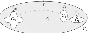
LetGbe a bounded multiply connected region of connectivitym 1≥1 with 0∈G. The boundaryΓ : ∂G m_j₀Γj consists ofm1 smooth closed Jordan curvesΓ0,Γ1, . . . ,

ΓmwhereΓ0contains the other curvesΓ1, . . . ,ΓmseeFigure 1. The complementG−:C\G ofG with respect toCconsists ofm1 simply connected components G0, G1, . . . , Gm. The componentsG1, . . . , Gmare bounded and the componentG0 is unbounded where ∞ ∈ G0.

We assume that the orientation of the boundary Γ is such that G is always on the left of Γ. Thus, the curves Γ1, . . . ,Γm always have clockwise orientations and the curve Γ0

has a counterclockwise orientation. The curve Γj is parametrized by a 2π-periodic twice continuously diﬀerentiable complex functionηjtwith nonvanishing first derivative

˙

ηjt

dηjt

dt /0, t∈Jj: 0,2π, j0,1, . . . , m. 2.1

The total parameter domain J is the disjoint union of the intervals Jj. We define a parametrization of the whole boundaryΓas the complex functionηdefined onJby

ηt:

⎧ ⎪ ⎪ ⎨ ⎪ ⎪ ⎩

η0t, t∈J0,

.. .

ηmt, t∈Jm.

(3)

Γm Γ0

Γ1 Γ2

Gm

G0

G1

G2

G

Figure 1:A bounded multiply connected regionGof connectivitym1.

LetHbe the space of all real H ¨older continuous functions on the boundaryΓ. In view of the smoothness ofη, a functionφ∈Hcan be interpreted viaφt:φηt,t∈J, as a real H ¨older continuous 2π-periodic functionsφtof the parametert∈J, that is,

φt:

⎧ ⎪ ⎪ ⎨ ⎪ ⎪ ⎩

φ0t, t∈J0,

.. .

φmt, t∈Jm,

2.3

with real H ¨older continuous 2π-periodic functionsφjdefined onJj, and vice versa. So, here and in what follows, we will not distinguish betweenφηtandφt.

The subspace ofHwhich consists of all piecewise constant functions defined onΓwill be denoted byS, that is, a functionh∈Shas the representation

ht:

⎧ ⎪ ⎪ ⎨ ⎪ ⎪ ⎩

h0, t∈J0,

.. .

hm, t∈Jm,

2.4

whereh0, . . . , hmare real constants. For simplicity, the functionhwill be denoted by

ht h0, . . . , hm. 2.5

In this paper we will assume that the function Ais the continuously diﬀerentiable complex function

At:e−iθt ηt, 2.6

whereθis the real piecewise constant function

θt θ0, . . . , θm, 2.7

(4)

The generalized Neumann kernel formed withAis defined by

Ns, t: 1

π Im

As At

˙

ηt

ηt−ηs . 2.8

We define also a real kernelMby

Ms, t: 1

π Re

As At

˙

ηt

ηt−ηs . 2.9

The kernelN is continuous and the kernelMhas a cotangent singularity typesee1for more details. Hence, the operator

Nμs:

J

Ns, tμtdt, s∈J, 2.10

is a Fredholm integral operator and the operator,

Mμs:

J

Ms, tμtdt, s∈J, 2.11

is a singular integral operator.

The solvability of boundary integral equations with the generalized Neumann kernel is determined by the indexwinding number in other terminologyof the functionAsee1. For the functionAgiven by2.6, the indexκjofAon the curveΓjand the indexκ

_m

j0κj ofAon the whole boundaryΓare given by

κ01, κj0, j1, . . . , m, κ1. 2.12

Although the functionAtin2.6is diﬀerent from the functionAtin2, Equation

11, both functions have the same indices. So by using the same approach used in

2, we can prove that the properties of the generalized Neumann kernel proved in 2, except Theorem 8, Theorem 10, and Corollary 2, are still valid for the generalized Neumann kernel formed with the function Atin 2.6 see5. Numerical evidence show that 2, Theorem 8, which claims that the eigenvalues of the generalized Neumann kernel lies in

−1,1, is no longer true for the functionAtin2.6 seeFigure 3.

Theorem 2.1see5. For a given functionγ∈H, there exist unique functionsh∈Sandμ∈H

such that

Af γh iμ 2.13

is a boundary value of a unique analytic functionfzinG. The functionμis the unique solution of the integral equation

(5)

and the functionhis given by

h

Mμ−I−Nγ

2 . 2.15

3. The Mixed Boundary Value Problem

LetSdandSnbe two subsets of the set{0,1, . . . , m}such that

Sd/∅, Sn/∅, Sd∪Sn{0,1, . . . , m}, Sd∩Sn ∅. 3.1

We will consider the following class of mixed boundary value problems. Find a real function

uinGsuch that

Δu0, on G, 3.2a

uφj, on Γj forj∈Sd, 3.2b

∂u

∂n φj, on Γj forj∈Sn, 3.2c

wherenis the unit exterior normal toΓ.

The problem3.2a,3.2b, and3.2creduces to the Dirichlet problem forSn ∅and to the Neumann problem for Sd ∅. Both problems have been considered in 2. So we have assumed in this paper thatSn/∅andSd/∅. The mixed boundary value problem3.2a,

3.2b, and3.2cis uniquely solvable. Its unique solutionucan be regarded as a real part of an analytic functionFinGwhich is not necessairly single-valued. However, the functionF

can be written as

Fz fz−

m

j1

ajlog

z−zj

, 3.3

wherefis a single-valued analytic function inG, eachzjis a fixed point inGj,j 1,2, . . . , m; and a1, . . . , am are real constants uniquely determined by φ see 12, page 145 and 13, page 174. Without los of generality, we assume that Imf0 0. The constantsa1, . . . , am are chosen to ensure thatsee14, page 222and15, page 88

Γk

fηdη0, k1,2, . . . , m, 3.4

that is,ajare given bysee2

aj 1 2πi

Γj

(6)

We define a real constanta0by

a0:−

m

j1

aj. 3.6

Hence, we have

a0−

m

j1

aj − m

j1

1 2πi

Γj

Fηdη− 1

2πi

ΓF

_η_dη 1

2πi

Γ0

Fηdη. _3.7

Since1/2πi_ΓFηdη0, we obtain

a0

1 2πi

Γ0

Fηdη. 3.8

The Dirichlet boundary condition is a special case of the Riemann-Hilbert boundary condition. The Neumann boundary condition also can be reduced to a Riemann-Hilbert boundary condition by using the Cauchy-Riemann equations and integrating along the boundaryΓj for j ∈ Sn. Let Tζ be the unit tangent vector and nζ be the unit external normal vector toΓatζ∈Γ. Let alsoνζbe the angle between the normal vector nζand the positive real axis, that is, nζ eiνζ. Then,

eiνηt−iTηt−iη˙t ˙

ηt. 3.9

Thus

∂u

∂n ∇u·ncosν

∂u ∂x sinν

∂u ∂y Re

eiν

∂u ∂x−i

∂u

∂y . 3.10

Sinceuz ReFz, then by the Cauchy-Riemann equation, we have

Fz ∂uz ∂x −i

∂uz

∂y . 3.11

Thus3.10becomes

Re−i ˙ηFη˙∂u

∂n. 3.12

Let the boundary value of the multivalued analytic functionFbe given by

(7)

Then the functionFzis a single-valued analytic function and has the boundary value

˙

ηFψiϕ. 3.14

Letθtbe the real piecewise constant function

θt

⎧ ⎨ ⎩

0, t∈Jj, j∈Sd,

π

2, t∈Jj, j∈Sn.

3.15

Hence, the boundary values of the functionFzsatisfy on the boundaryΓ

Ree−iθt_F_η_t_φ_t_, _3.16

where

φt

⎧ ⎨ ⎩

φjt, t∈Jj, j∈Sd,

ϕjt, t∈Jj, j∈Sn,

3.17

and fort∈Jjandj∈Sn, the functionϕjtis known and is given by

ϕ_jt Re−i ˙ηjtF

ηjt

φjtη˙jt, t∈Jj, j∈Sn. 3.18

The functionsφjtforj∈Sd∪Snare given by3.2band3.2c. The functionϕjtcan be then computed fort∈Jjandj ∈Snby integrating the functionϕ_jt. Then, it follows from3.3,

3.16, and3.17that the the functionfzis a solution of the Riemann-Hilbert problem

Ree−iθtfηtφt

m

k1

akRe

e−iθtlogηt−zk

. 3.19

Since

logηt−zk

logηt log

1− zk

ηt , 3.20

then, in view of3.6, the boundary condition3.19can be written as

Ree−iθt_f_η_t_φ_t m k0

(8)

where

γ0t −Ree−iθtlogηt, γkt Re

e−iθtlog

1− zk

ηt , 3.22

fork1,2, . . . , m.

In view of3.5,3.8, and3.18, the constantsakare known fork∈Snand are given by

ak 1 2π

Jk

φktη˙ktdt, k∈Sn. 3.23

Fork ∈Sd, the real constantsakare unknown. Thus, the boundary condition3.19can be written as

Ree−iθtfηtψt

k∈Sd

akγkt, t∈J, _3.24

where the functionψtis known and is given by

ψt

⎧ ⎪ ⎨ ⎪ ⎩

φjt

k∈Sn

akγjkt, t∈Jj, j∈Sd,

ϕjt

k∈Sn

akγ_jkt, t∈Jj, j∈Sn.

3.25

It is clear that the functionψjtis known explicitly fort∈Jjwithj∈Sd. However, fort∈Jj withj∈Snit is required to integrateϕ_jtto obtainϕjt.

The functionϕjtis not necessary 2π-periodic. Numerically, we prefer to deal with periodic functions. So we will not computeϕjtdirectly by integrating the function ϕ_jt. Instead, we will integrate the function

ψ_jt φjtη˙jt

k∈Sn

ak

d dtγ

k

j t. 3.26

By the definitions of the constantsakand the functionsγk, we have

2π

0

ψ_jtdt0, 3.27

which implies that the functionψjt ϕjt k∈Snakγ

k

j tis always 2π-periodic. So, for

t∈Jjwithj∈Sn, we write the functionψ_jtusing the Fourier series as

ψ_jt

∞

i1

a_ijcosit

∞

i1

(9)

Then the functionψjtis given fort∈Jjwithj∈Snby

ψjt ψjt cj, 3.29

wherecjis undetermined real constant and the functionψjtis given by

ψjt

∞

i1

a_ij i sinit−

∞

i1

b_ij

i cosit, t∈Jj, j ∈Sn. 3.30

Hence, the boundary condition3.24can be then written as

Ree−iθtfηtγt ht

k∈Sd

akγkt, t∈J, _3.31

wherehtis the real piecewise constant function

ht

0, t∈Jj, j∈Sd,

cj, t∈Jj, j∈Sn,

3.32

and the functionγtis given by

γt

⎧ ⎨ ⎩

φjt

k∈Sn

akγjkt, t∈Jj, j∈Sd,

ψjt, t∈Jj, j∈Sn.

3.33

Letc:f0 unknown real constantandgzbe the analytic function defined onG

by

gz: fz−c

z , z∈G. 3.34

Thus the functiongzis a solution of the Riemann-Hilbert problem

ReAtgηtγt ht

j∈Sd

ajγjt, t∈J, _3.35

where the functionAtis given by2.6and the functionhtis defined by

(10)

Let μt : ImAtgηt, then the boundary value of the function gzis given on the boundaryΓby

Atgηtγt ht

j∈Sd

ajγjt iμt, t∈J, _3.37

whereγ,γjare knowns andh,μare unknowns.

4. The Solution of the Mixed Boundary Value Problem

Letμand letμj_for_j_∈_S

dbe the unique solutions of the integral equations

I−Nμ−Mγ, I−Nμj−Mγj, 4.1

andh,hj_{be given by}

h

Mμ−I−Nγ

2 , h

j

Mμj₋_I₋_N_γj

2 . 4.2

Then, it follows fromTheorem 2.1that

Atgηtγhiμ

j∈Sd

aj

γjhjiμj _4.3

is the boundary value of an analytic functiongz. Since the unknown functionsμandhin

3.37are uniquely determined by the known functionsγandγj_for_j _∈_S_{d, it follows from}

3.37and4.3that

μt μt

j∈Sd

ajμjt, _4.4

ht ht

j∈Sd

ajhjt. _4.5

In view of3.15,3.32, and3.36, the functionhtis given by

ht

−c, t∈Jj, j∈Sd,

cj, t∈Jj, j∈Sn.

(11)

Thus, we have from4.5,3.23, and3.6the linear system

ht−

j∈Sd

ajhjt ht, _4.7a

j∈Sd

aj−

j∈Sn

aj, _4.7b

ofm2 equations inm2 unknownsc,ajforj∈Sdandcjforj∈Sn.

By solving the linear system4.7aand4.7b, we obtain the values of the constantsaj and the functionht. Then, we obtain the functionμfrom4.4. Consequently, the boundary value of the functiongis given by

Atgηtγt ht iμt, t∈J, 4.8

where

γt γt

j∈Sd

ajγjt, t∈J. _4.9

The function gz can be computed for z ∈ G by the Cauchy integral formula. Then the functionfzis given by

fz czgz. 4.10

Finally, the solution of the mixed boundary value problem can be computed fromuz

ReFzwhereFzis given by3.3.

5. Numerical Implementations

Since the functionsAjandηj are 2π-periodic, the integrands in the integral equations4.1 are 2π-periodic. Hence, the most efficient numerical method for solving 4.1 is generally the Nystr öm method with the trapezoidal rule see e.g., 16, page 321. We will use the trapezoidal rule with n an even positive integer equidistant node points on each boundary component to discretize the integrals in4.1. If the integrands in4.1arektimes continuously differentiable, then the rate of convergence of the trapezoidal rule isO1/nk_. For analytic integrands, the rate of convergence is better than 1/nk_{for any positive integer}

k see e.g., 17, page 83. The obtained approximate solutions of the integral equations converge to the exact solutions with a similarly rapid rate of convergence see e.g., 16, page 322. Since the smoothness of the integrands in 4.1depends on the smoothness of the functionηt, results of high accuracy can be obtained for very smooth boundaries.

(12)

By solving the linear systems, we obtain approximations toμandμj_for_j_∈_S

dwhich give approximations tohandhj_for_j_∈_S

dthrough4.2. By solving4.7aand4.7bwe get approximations to the constantsc,ajforj∈Sdandcjforj∈Sn. These approximations allow us to obtain approximations to the boundary value of the functiongzfrom4.8. The values ofgzforz∈Gwill be calculated by the Cauchy integral formula. The approximate values of the functionfzare then computed from4.10. Finally, in view of3.3, the solution of the mixed boundary value problem can be computed from

uz ReFz Refz−

m

j1

ajlogz−zj. 5.1

In this paper, we have considered regions with smooth boundaries. For some ideas on how to solve numerically boundary integral equations with the generalized Neumann kernel on regions with piecewise smooth boundaries, see18.

6. Numerical Examples

In this section, the proposed method will be used to solve two mixed boundary value problems in bounded multiply connected regions with smooth boundaries.

Example 6.1. In this example we consider a bounded multiply connected region of connectivity 4 bounded by the four circlesseeFigure 2a

Γ0:η0t 12eit,

Γ1:η1t 10.25e−it,

Γ2:η2t 1i0.25e−it,

Γ3:η2t 1−i0.25e−it,

6.1

where 0≤t≤2π.

We assume that the condition on the boundariesΓ0,Γ1is the Neumann condition and

the condition on the boundariesΓ2,Γ3is the Dirichlet condition. The functionsφj in3.2a, 3.2b, and3.2care obtained based on choosing an exact solution of the form

uz Rez−13. 6.2

This example has been considered in9, page 894using the regularized meshless method. The domain here is shifted by one unit to the right to ensure that 0 ∈ G. To compare our method with the method presented in9, we use the same error norm used in9, namely,

₂_π

0

u10.5eis₋_u n

(13)

2

1

0

−1

−2

−1 0 1 2 3

a

3 1

−3 −3

−1 −1

1 3

b

Figure 2:The regions ofExample 6.1aand Example 2b.

1

0.5

0

−0.5

−1

0 0.5 1 1.5 2

a

1

0.5

0

−0.5

−1

0 0.5 1 1.5 2

b

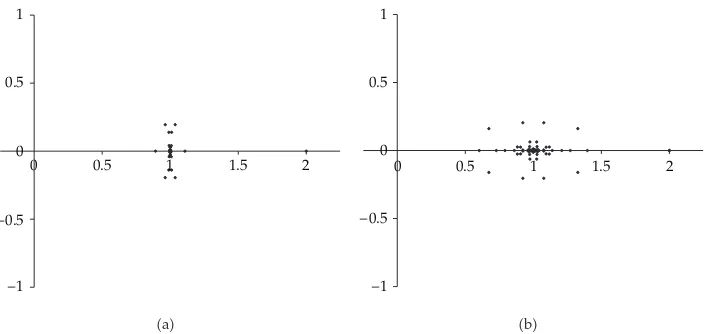
Figure 3: The eigenvalues of the coeﬃcient matrix of the linear systems obtained by discretizing the

integral equations4.1withn128 forExample 6.1aand withn256 forExample 6.2b.

(14)

100 ₁₀1 ₁₀2 ₁₀3

100

10−5

10−10

10−15

10−20

Error norm

Total number of collocation points

a

100 ₁₀1 ₁₀2 ₁₀3

100

10−5

10−10

10−15

10−20

Error norm

Total number of collocation points

b

Figure 4:The error norm6.3for Example 1aand the error norm6.6forExample 6.2bversus the

total number of node points.

×10−14

6 4 2 0 −2 2 1 0 −1 −2 y_-axis x-axis −1 0 1 2 3 | u ( z ) − un ( z ) | a

×10−14

4 2 0 2 0 −2 −4 y_-axis x-axis

−3 −2 −1 0 1 2 | u ( z ) − un ( z ) | b

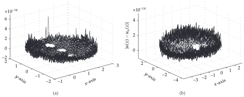
Figure 5:The absolute error|uz−unz|for the entire domain obtained withn64 forExample 6.1a

and withn256 forExample 6.2b.

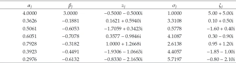
Example 6.2. In this example we consider a bounded multiply connected region of connectivity 7seeFigure 2b. The boundaryΓ ∂Gis parametrized by

ηjt zjeiσj

αjcostiβjsint

, j0,1, . . . ,6, 6.4

where the values of the complex constantszjand the real constantsαj,βj,σjare as inTable 1.

The region in this example has been considered in2,19,20for the Dirichlet problem and the Neumann problem. In this example, we will consider a mixed boundary value problem where we assume that the condition on the boundaries Γ0,Γ1,Γ2, and Γ3 is the

(15)

Table 1:The values of constantsαj,βj,zj,σj, andζjin6.4.

j αj βj zj σj ζj

0 4.0000 3.0000 −0.5000−0.5000i 1.0000 5.005.00i

1 0.3626 −0.1881 0.16210.5940i 3.3108 0.100.50i

2 0.5061 −0.6053 −1.70590.3423i 0.5778 −1.600.40i

3 0.6051 −0.7078 0.3577−0.9846i 4.1087 0.30−0.90i

4 0.7928 −0.3182 1.00001.2668i 2.6138 0.951.20i

5 0.3923 −0.4491 −1.9306−1.0663i 4.4057 −1.85−1.00i

6 0.2976 −0.6132 −0.8330−2.1650i 5.7197 −0.80−2.10i

condition. The functionsφj in3.2a,3.2b, and3.2care obtained based on choosing an exact solution of the form

uz 12Re

1

z−ζ0 6

j1

j−7/2logz−ζj2

, 6.5

where the values of the complex constantsζjare as inTable 1. For the error, we use the error normseeFigure 4b:

₂_π

0

u−0.35−0.35i2.7eis−un

−0.35−0.35i2.7eis2ds. 6.6

The absolute errors |uz− unz| for selected points in the entire domain are plotted in Figure 5b.

7. Conclusions

A new uniquely solvable boundary integral equation with the generalized Neumann kernel has been presented in this paper for solving a certain class of mixed boundary value problem on multiply connected regions. Two numerical examples are presented to illustrate the accuracy of the presented method.

The presented method can be applied to mixed boundary value problem with both the Dirichlet condition and the Neumann condition on the same boundary component

Γk. For this case, the function At is discontinuous on Jk, where At ηkt on the part of Γk corresponding to the Dirichlet condition and At −iηkt on the part of Γk corresponding to the Neumann condition. Hence, the Riemann-Hilbert problem3.35will be a problem with discontinuous coefficientAt. The solvability of Riemann-Hilbert problems with discontinuous coefficients is different from the ones with continuous coefficientssee e.g.,6, page 449and 13, page 271. Furthermore, the discontinuity of the functionAt

implies that we cannot apply the theory of the generalized Neumann kernel developed in

(16)

Acknowledgments

The authors would like to thank the anonymous referees for suggesting several improve-ments. This work was supported in part by the Deanship of Scientific Research at King Khalid University through Project no. KKU-SCI-11-022. This support is gratefully acknowledged.

References

1 R. Wegmann and M. M. S. Nasser, “The Riemann-Hilbert problem and the generalized Neumann

kernel on multiply connected regions,” Journal of Computational and Applied Mathematics, vol. 214, no. 1, pp. 36–57, 2008.

2 M. M. S. Nasser, A. H. M. Murid, M. Ismail, and E. M. A. Alejaily, “Boundary integral equations

with the generalized Neumann kernel for Laplace’s equation in multiply connected regions,” Applied

Mathematics and Computation, vol. 217, no. 9, pp. 4710–4727, 2011.

3 M. M. S. Nasser, “A boundary integral equation for conformal mapping of bounded multiply

connected regions,” Computational Methods and Function Theory, vol. 9, no. 1, pp. 127–143, 2009.

4 M. M. S. Nasser, “Numerical conformal mapping via a boundary integral equation with the

generalized Neumann kernel,” SIAM Journal on Scientific Computing, vol. 31, no. 3, pp. 1695–1715, 2009.

5 M. M. S. Nasser, “Numerical conformal mapping of multiply connected regions onto the second,

third and fourth categories of Koebe’s canonical slit domains,” Journal of Mathematical Analysis and

Applications, vol. 382, no. 1, pp. 47–56, 2011.

6 F. D. Gakhov, Boundary Value Problems, Pergamon Press, Oxford, UK, 1966.

7 R. Haas and H. Brauchli, “Fast solver for plane potential problems with mixed boundary conditions,”

Computer Methods in Applied Mechanics and Engineering, vol. 89, no. 1–3, pp. 543–556, 1991.

8 R. Haas and H. Brauchli, “Extracting singularities of Cauchy integrals—a key point of a fast solver

for plane potential problems with mixed boundary conditions,” Journal of Computational and Applied

Mathematics, vol. 44, no. 2, pp. 167–185, 1992.

9 K. H. Chen, J. H. Kao, J. T. Chen, D. L. Young, and M. C. Lu, “Regularized meshless method for

multiply-connected-domain Laplace problems,” Engineering Analysis with Boundary Elements, vol. 30, no. 10, pp. 882–896, 2006.

10 H. S. Ho and D. Gutierrez-Lemini, “A general solution procedure in elastostatics with

multiply-connected regions with applications to mode III fracture mechanics problems,” Acta Mechanica, vol. 44, no. 1-2, pp. 73–89, 1982.

11 E. Dontov´a, M. Dont, and J. Kr´al, “Reflection and a mixed boundary value problem concerning

analytic functions,” Mathematica Bohemica, vol. 122, no. 3, pp. 317–336, 1997.

12 S. G. Mikhlin, Integral Equations and Their Applications to Certain Problems in Mechanics, Mathematical

Physics and Rechnology, Pergamon Press, New York, NY, USA, 1957, Translated from the Russian by

A. H. Armstrong.

13 N. I. Muskhelishvili, Singular Integral Equations, Wolters-Noordhoﬀ, Leyden, Mass, USA, 1972,

English translation of Russian edition 1953.

14 P. Henrici, Applied and Computational Complex Analysis, Vol. 3, John Wiley & Sons, New York, NY, USA,

1986.

15 S. G. Krantz, Geometric Function Theory: Explorations in Complex Analysis, Birkh¨auser, Boston, Mass,

USA, 2006.

16 K. E. Atkinson, The Numerical Solution of Integral Equations of the Second Kind, vol. 4, Cambridge

University Press, Cambridge, UK, 1997.

17 A. R. Krommer and C. W. Ueberhuber, Numerical Integration on Advanced Computer Systems, vol. 848,

Springer, Berlin, Germany, 1994.

18 M. M. S. Nasser, A. H. M. Murid, and Z. Zamzamir, “A boundary integral method for the

Riemann-Hilbert problem in domains with corners,” Complex Variables and Elliptic Equations, vol. 53, no. 11, pp. 989–1008, 2008.

19 A. Greenbaum, L. Greengard, and G. B. McFadden, “Laplace’s equation and the Dirichlet-Neumann

(17)

20 J. Helsing and E. Wadbro, “Laplace’s equation and the Dirichlet-Neumann map: a new mode for Mikhlin’s method,” Journal of Computational Physics, vol. 202, no. 2, pp. 391–410, 2005.

21 R. Wegmann, A. H. M. Murid, and M. M. S. Nasser, “The Riemann-Hilbert problem and the

(18)

Submit your manuscripts at

http://www.hindawi.com

Hindawi Publishing Corporation

http://www.hindawi.com Volume 2014

Mathematics

Journal of

Mathematical Problems in Engineering

Hindawi Publishing Corporation http://www.hindawi.com

Differential Equations

International Journal of

Volume 2014

http://www.hindawi.com Volume 2014 Hindawi Publishing Corporationhttp://www.hindawi.com Volume 2014

http://www.hindawi.com Volume 2014 Mathematical PhysicsAdvances in

Complex Analysis

Journal of Hindawi Publishing Corporation

Optimization

Journal of Hindawi Publishing Corporation

Combinatorics

http://www.hindawi.com Volume 2014 International Journal of

Journal of

Function Spaces

Abstract and Applied Analysis Hindawi Publishing Corporation

International Journal of Mathematics and Mathematical Sciences

The Scientific

World Journal

Discrete Dynamics in Nature and Society Hindawi Publishing Corporation

Discrete Mathematics

Journal of

http://www.hindawi.com Volume 2014 Hindawi Publishing Corporationhttp://www.hindawi.com Volume 2014

A boundary integral equation with the generalized neumann kernel for a mixed boundary value problem in unbounded multiply connected regions

Research Article