A finite difference technique for solving incompressible fluid flow and energy equations on distributed parallel computer system

A FINITE DIFFERENCE TECHNIQUE FOR SOLVING

INCOMPRESSIBLE FLUID FLOW AND ENERGY

EQUATIONS ON DISTRIBUTED PARALLEL

COMPUTER SYSTEM

Bukhari bin Manshoor

Mat Nawi Wan Hassan, Prof. Dr

Norma Alias, Dr.

Faculty of Mechanical Engineering and

Manufacturing, KUiIIHO Batu Pahat,

Johor

FacuIty of Mechanical Engineering,

VIM Skudai, Johor

07-5534755

Faculty of Science, VIM Skudai, Johor

07-5534416

07-4537828

[email protected]

is paper is concemed with the development of an efficient erne for solving the finite difference Navier-Stokes and energy ations using distributed parallel computer system. The 'merical procedure is based on SIMPLE (Semi Implicit Method Pressure Link Equations) developed by Spalding. The Iveming equations are transformed into finite difference forms ing the control volume approach. The hybrid scheme which is . bination of the central dilIerence and up wind scheme is used obtaining a profile assumption for parameter variations ,en the grids points. Parallelization method used on this ributed parallel computer system is Domain Decomposition :thod (DDM). The accuracy of the parallelization method is e by comparing with a benchmark solution of a standardized ,Iern related to the two dimensional buoyancy flow in a square :Iosure. The results shown that the distributed parallel puter system will reduced an execution time to solve the Iblem about

70°.

compared to the serial computer.

!ywords

PLE algorithm. Parallel Algorithm. Domain Dccomposition 00, Navier-Stokes Equations.

equations goveming the lluid dynamics and energy flow have know for the most parl for morc than a century and yet have 'nued to defy analytical solution. Instead their solutions have

:Iy

been obtained by experimental simulations in wind ,cis, water tables aud shock hlbes [4]. Novv with the ability of ced scientitic computer such as distributed parallel puter system. the equations can be solved using the methods Irnputational fluid dynamic (CFD). Now. it surprising that, dynamics and heat transfer are contributing to and benefiting . current development in finite difference numerical analysis.

nt years. several finite difference schemes have been d and develop. Some methods have used the primitive les, while some have solved the equations in terms of

:ity and stream function as the dependent variables. The ing equations are often transformed into the non­ sionallorm. The advantage is that it is more ~onvenientto with dimensionless variables. The characteristi~parameter

40

[email protected]

such as Reynold number. Prandt number and Rayleigh number can be varied independently. Furthermore. by non­ dimensionalising the equations, the flow parameters such as velocity and temperature are normalized so that their values can be adjusted to fall between certain prescribed limits. A number of general purpose computer programs using finite difference methods have been developed. Some of these programs using serial computer have relied on works of the Argonne National Laboratory Group, IIIinious. USA [5] and methods based on the works at Imperial College. London [8].

This paper deals with a development of an efficient scheme tor solving the finite difference Navier-Stokes and energy equations using distributed parallel computer system. The numerical procedure is based on SIMPLE (Semi Implicit Method for Pressure Link Equations) developed by Spalding [2]. As we know. the analysis of an incompressible flow become more complicated and need a high performance computer to solve the problem. One of the problem during to solve the complicated problem on incompressible flow is time constraint. More complicated of the problem means more time should be spend to solve the problem.

To overcome this problem. parallel computer was used and to determine the performance of this parallel computations. the corresponding parallel algorithms was developed and it based on method of parallelization there is Domain Decompositions Method. As the number of the nonlinear simultaneous equations formed after diseretisation of the modelling equations is large, an iterative technique is used to update the flow variables. Control volume approach is selected and the matrix formed used to solved using matrix tri-diagonal solver. At the end of this project. the result of simulation using distributed parallel computer system are in terms of how the parallel computer can reduced an execution time compare with the serial computer are presented and discussed.

2. NUMERICAL ANALYSIS

2.1 Governing equations

communication process between a data or function that will be send or receive. According to the pseudo code solution in Figure 2, the communication process occurs between the master and slave during to their sending and receiving the data or function.

find out iff am MASTER or SL4 VES iff am MASTER

lnrtial/Ze array

send each SL4 VES startmg mfo and subarray do until all SL4VES converge

gather from all SL4/c_{ES convergence data}

broadcast to all SL4VES cOnJ'ergence signal end do

receive results from each SL4 VE else

if

1am SL4I'E

receive from AfASTER starting mfrJ and subarray

do untl! solutIOn converged update time

send neighbors my border infO receive from neighbors their border mfo

update my portion ofsolutIOn array

determine ifmy solutIOn has converged send A1ASTER convergence data receive from MASTER convergence ."gnal end do

send AL4STER results endif

Figurl.' 2. Pseudo code solution

3.2 Communication

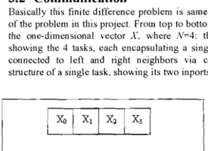
Basically this finite difference problem is same with the solution of the problem in this project. From top to bottolll of the Figure 3~

the one-dimensional vector X, where N=4: the task structure, showing the 4 tasks, each encapsulating a single data value and connected to left and right neighbors via channels: and the structure of a single task, showing its two in ports and outports.

~

ro~(ID~~)~(QJ)

"!\t;l:"

_~----....

"right"

---.t'/~\,-....

.--_.\~)

..

----­

"

..

_ /

Figure 3. A parallel algorithms for the finitl' difference problem

We first consider a one-dimensional finite difference problem, in h h v(o) - ' N d \-(T) whIC· we ave a vector A ot sIze an IlIUSt compute· , where;

O<i<N-1.

O~t<T

:X,II<I) =

X,II)+2X,(t)+X>+1~

4

That is, we must repeatedly update each element of X, with no element being updated in step t+ 1 until its neighbors have been updated in step t. A parallel algorithm for this problem creates N

tasks. one for each point in X. The ith task is gi ven the value

X

IO _{)and is responsible for computing, in T steps. the}

valuesx,I'I. X,III, ... , X,IT).

Hence, at step I, it must obtain the values

X

II) and

X

(I) from

I-I /.... 1

tasks i-I and i+1. We specify this data transfer by defining channels that link each task with "left" and "right" neighbors, as shown in Figure 3. and requiring that at step I, each task i other than task 0 and task N-l

i. sends its data x(T)on its left and right outports, I

ii. receives

Xi./')and X,}I

from its left and right and

iii. use these values to com pute

X

(1+1).

1

Notice that the N tasks can execute independently. with the only constraint on execution order being the synchronization enforce by the receive operations. This synchronization ensures that n data value is updated at step f+ 1 until the data values i neighboring tasks have been updated at step I. Hence, execution i

deterministic.

C broadcast data to slaves

call pvmfimtsend (PVMDEFAULT, info) call pvmfpack (fNTEGER4, nproc, 1, 1, info) call pvnifpack (fNTEGER4, tlds, nproc, 1, mfo) call pvmfPack (fNTEGER4, n, 1, 1, mfo) call pvmfPack (RE4L8, data, n, 1, info) msgtype = 1

call pvmfmcast Inproc, tids, msgtype, infO)

C wait for results from slaves

msgtype =2

do 30 1= l,nproc

call pvmfrecv 1-1, msgtype, mfo)

call pvmjimpack IINTEGER4, who, 1, 1, info) call pvmfunpack lRE4L8, resultlwho+ 1), 1, 1, info) if Iwho.eq. 0)

then

wme 1*,1000) resultlwho+ 1), who, Inroc-1) else

w/'lte (*,1000) resultlwho+ l), who, 2*(who-l) 30 continue

Figure 4. Algorithm master to send and rl'ceive from slaves.

o :n N Ie le ,m ng as ler rts,

msgtype = 1

call pvmfrecv (mtid, msgtype, mfo)

callpvmjimpack (1NTEGER4. nproc, 1, 1, info) call pvmjUnpack (1NTEGER4, tids, nproc, 1, info) . call pvmjUnpack (1NTEGER4, n, 1, 1, mfo)

call pvmjUnpack (REAL8, data, n, 1, info) determine which slave J'm (O... nproc-1)

do calculation wIth the data

send the result to the mas ter

call pvmfinitsend (PVMDEFAULT, info) callpvmfpack(1NTEGER4, me, 1, 1, mfo) callpvmfpack(REAL8, result, 1. 1. mfo} msgtype =2

call pvmftend (mtid, msgtype, info)

re 5. Algorithm sIan's to receive and send data from and master.

figure 4 and 5 above showed the algorithms for the sending and iving data from master and slaves.

4. DISCUSSION

4.1 Validation of the Results

'able I to 3 compared the results from the present simulation with the literature results obtained by de Vahl Davis [2]. The JeSUits of de Vahl Davis are the standard against which all other

~eshave been evaluated. Maximum horizontal velocity on the lertical midplane of the cavity, Umax, maximum vertical velocity

CllI the horizontal midplane of the cavity, Vmax, and an average of

Nusselt number was compared at Rayleigh numbers of 10J, 10'.

101 and 106 The comparison was done between the benchmark ICSUlts obtained by de Vahl Davis which in serial processor and dte present study that is simulation using serial processor and parallel processor or parallel computer.

From the tables. it showed that all these results are in excellent _ 'eement with the benchmark results of de Vahl Davis, Percentage error for the three methods of solution is below than 3% compare with benchmark result. Besides that. the result that

was

showed in the forms of contour maps of non-dimensional temperature and velocities also was compared with the results that obtained by de Vahl Davis.

Table 1. Comparison of the numerical result of present study for Umax

Ra 103 10' 10' 10'

G. de Vahl Davis 3.649 16.193 34.620 64.593

Presenl study:

i) Serial processor 3.652 16.163 34.871 65.812

0/0 error 0.082 % 0.185 % 0.725 % 1.880 %

ii)Parallel processor 3.592 16.376 34.852 65.847

°

10 error 1.560 % 1.131 % 0.670 % 1.941 %

Table 2. Comparison of the numerical result of present study for V""",

Ra )03 10'

105

106

G. de Vahl Davis 3.697 19.167 68.590 216.360

Presenl study:

i) Serial processing 3.704 19.675 69.482 220.641

°/0 error 0.189% 2.650 % 1.300 % 1.978 %

ii)Parallel processing 3.715 19.642 69.680 221.282

% error 0.487 % 2.478 % 1.589 % 2.275 %

Table 3. Comparison of the numerical result of present study for

Nu

Ra 103

10' 10' 10'

G. de Vahl Davis 1.118 2.243 4.519 8.800

Present study:

i) Serial processing 1.120 2.282 4.583 8.983

0/0 error 0.23 % 1.74% 1.42 % 2.08 %

ii)Parallel processing 1.123 2.272 4.594 9.008

0/0 error 0.47% 1.31 % 1.67 % 2.36 %

4.2 Parallel Computing Results

In order to achieve the objective of this project. parallel execution time was studied to determine the performance of the parallel computations. Two methods of solution there are serial computation and parallel computation were used during to obtain the results of the simulation. Table 4 showed the results for both methods of computational solution in term of execution time. Table 5 was showed the tabulated results of computational time and communication time for parallel with domain decomposition method.

Table 4. Execution time for three computational solutions

Ra Sequential time Parallel time

(tS"'l) (tp)

10J 32.8 s 9.43 s

10' 135.75 s 41.39 s

lOS

_{2040.26 s 612.06 s}

106 163602.04 s 49080.61 s

Table 5. Computational and communication time for parallel computation

Ra tcamp tcomm tp

103 8.41 s 1.02 s 9.43 s

10

4 34.62 s 6.78 s 41.39 s

10

5 522.82 s 89.24 s 612.06 s

10

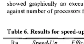
6 41923.02 s 7157.60s 49080.61 s

Other parameter that was used to measure a performance of parallel computations is speed-up and efficiency. From the speed­ up, we know that how fast the parallel computer solves the problem under consideration. It is sometimes useful to know how long processors are being used on the computation. which can be found from the efficiency. Table 6 below was showed result for speed-up and efficiency for parallel methods. Figure 6, 7 and 8 showed graphically an execution time, speed-up and efficiency against number of processors for Ra~103 respectively.

Table 6. Results for speed-up and efficiency

Ra Speed-Up EffiCiency

103 3.478 86.95 %

104 3.279 81.97 %

105 3.333 83.32 %

106 _{3.333 83.32}

%

4.3 Discussions

From the results that were obtained. we can see that execution time for parallel computation was decrease compare with sequential computation. By using sequential computation, total execution time that we need to complete our simulation at Rayleigh number 106 is 163602.04 seconds or 2726.7 minutes or 45.45 hours. For parallel computation. we were reduced an execution time for the simulation at Rayleigh number 106 to 49080.61 seconds or 818.01 minutes or 13.63 hours. Compare for both methods of simulations, we got the parallel computation with domain decomposition method is more successful for solve this problem with reducing about 70% of execution time.

From the Figure 6 to 8. we can see an effect of number of processors in parallelization to the execution time. speed-up and efficiency. As we can see. the execution time will decrease with increasing of the number of processors. For the speed-up. it will increase with the increasing of the number of processors. However. the efficiency of a simulation was decrease with an increasing of the number of processors.

§ §

15

j

~

10J,~~~

~

_""'=

5 +-1---~cT

o

-I-I---~---~---c­

o

2 3

No of Processors

Figure

6.

Execution time against no. of processors for Ra

=

1

3.5

2.5 ~

~

2 ,,/

Q. 7

rJJ 15

0.5 +-~~~~~--~~~~--=

o -l-I~~~~~~~_~~_~===

o 0.5 15

I\b of Frocessors

Figure 7. Speed-Up against no. of processors for Ra =

ur

102

0.98

>0 0.96

g

~ 0.94

w 0.92

"

0.9

0.88

0.86

0 0.5 1 1.5 2 2.5

No of Ffocessocs

Figure 8. Efficiency against no. of processors for Ra = 103

5. CONCLUSION

A parallel algorithm has been developed to simulate incompressible flow for the problem of natural convection occurred in a square cavity with specified boundary conditi, The simulations of the incompressible flow using SIMP' method on parallel computer are agreement with the benchm result. Thus. the simulation is successful. Percentage errors for