ABSTRACT
BAN, DAEHYUN. Connectivity-Based Performance Analysis and Reliability Improvement Algorithms in Wireless Sensor, Mobile Networks and Smart-Grids. (Under the direction of Michael Devetsikiotis.)
This dissertation proposes network performance measurement methods and reliability im-provement algorithms in Wireless Sensor Networks (WSNs), mobile opportunistic networks and smart-grids, based on connectivity issues. In Electrical Engineering and Computer Science, these network categories have been received a high interest in a decade.
In the process of network analysis, it is important to understand and capture the network characteristics to induce valid analytical results. For sure, the property is not invariant to network categories and this acknowledgement lets me divide this dissertation into two broad parts, where one part is WSNs and mobile opportunistic networks and the other is smart-grids. The first part of this subject includes data network analysis. In WSNs, methods to extend the life-time of networks have been studied along with establishing its connectivity. These two have a trade-off, and balancing their performance is regarded as a challenging work. About the issue, this subject proposes an autonomous and distributed sensor sleep/awake control without losing algorithm simplicity. In mobile opportunistic networks, contact information among users is important as it provides chances to propagate contents. However, in general, mobile users spend their time under wide-area networks, such as 3G and 4G cellular networks. For this reason, it is required to determine the performance variation when those infrastructures are partly added to opportunistic content propagation. In addition, mobile devices such as smart phones, which suffer an energy constraint, may apply power-saving strategies. This subject also concerns the performance changes of age-sensitive content propagation when those strategies are used in mobile devices.
smart-grids, this subject considers centrality estimation methods to reveal network vulnerability. When the electric property is included to centrality, this subject shows that the measured centrality can be different a lot from ones from data network centrality. This explains a possible reasoning of cascading failure phenomena in power society. After that, the property is connected to the dynamics of electric generator, a physical grid component. In power system analysis, there exists a small-signal stability analysis to investigate generator dynamics. But, this incurs so high complexity that it is unfit for recent power grid trends, large-scale and complex interconnections. This subject proposes a complexity reduction method for generator dynamics analysis.
©Copyright 2012 by Daehyun Ban
Connectivity-Based Performance Analysis and Reliability Improvement Algorithms in Wireless Sensor, Mobile Networks and Smart-Grids
by Daehyun Ban
A dissertation submitted to the Graduate Faculty of North Carolina State University
in partial fulfillment of the requirements for the Degree of
Doctor of Philosophy
Electrical Engineering
Raleigh, North Carolina
2012
APPROVED BY:
Do Young Eun Wenye Wang
Rudra Dutta Michael Devetsikiotis
DEDICATION
BIOGRAPHY
ACKNOWLEDGEMENTS
I would like to acknowledge the inspirational instruction and guidance of my adviser, Dr. Michael Devetsikiotis, and the informational initial impetus of Dr. Do Young Eun. Both of these have given me a deep appreciation for the details of this subject.
I would also like to thank Dr. Wenye Wang, and Dr. Rudra Dutta, for being my advisory committee members and giving me many useful suggestions to finish this dissertation, and Dr. George Michailidis at University of Michigan, Ann Arbor, for advising my research on smart-grid modeling and analysis.
During my Ph.D. study, it was my pleasure to work with great research colleagues, Dr. Yuh-Ming Chiu, Dr. Han Cai, Dr. Sungwon Kim, Dr. Chul-Ho Lee, Boonyarith Saovapakhiran and Safak Bayram.
TABLE OF CONTENTS
List of Tables . . . ix
List of Figures . . . x
Chapter 1 Introduction . . . 1
1.1 Motivation and Overview . . . 1
1.1.1 Wireless Sensor Networks: Network Connectivity and Sensor Life-time . . 2
1.1.2 Mobile Opportunistic Networks: Realistic Version of Delay Tolerant Net-works (DTNs) . . . 3
1.1.3 Smart-Grids : Convergence Solutions between Power and Data Networks . 4 1.2 Contributions and Accomplishments . . . 5
1.2.1 Contributions . . . 5
1.2.2 Accomplishments . . . 5
1.3 Road-Map of This Dissertation . . . 6
Chapter 2 Balancing Network Connectivity and Life-Time of Wireless Sen-sors through Percolation and Consensus . . . 8
2.1 Chapter Abstract . . . 8
2.2 Chapter Introduction . . . 9
2.3 Problem Description . . . 11
2.3.1 Network Conditions and Assumptions . . . 11
2.3.2 Performance Measurement Metrics . . . 11
2.4 Controlling the Sleep/Awake of Sensors with Percolation Theory and Consensus Algorithm . . . 12
2.4.1 Matching Giant-Cluster Condition to Sensor Sleep/Awake . . . 12
2.4.2 Consensus Algorithm . . . 13
2.4.3 Sleep/Awake Control for Performance Balancing . . . 14
2.5 Simulations on Random Graphs . . . 16
2.5.1 Cluster Size Variation and Average Consensus . . . 17
2.5.2 The Proposed Sensor Sleep/Awake Method Tests . . . 18
2.6 Chapter Summary . . . 23
Chapter 3 Age-Sensitive Content Dissemination with Infrastructures in Mo-bile Opportunistic Networks . . . 24
3.1 Chapter Abstract . . . 24
3.2 Chapter Introduction . . . 25
3.3 Background and Problem Formulation . . . 27
3.3.1 Multi-Packet Delivery in Epidemic Routing . . . 27
3.3.2 Content Update Process . . . 28
3.3.3 Content Update Problem with Infrastructures . . . 29
3.4 Model and Analysis . . . 31
3.4.2 Age-distribution and Mean-Content Age . . . 33
3.4.3 Numerical Results and Freshness Enhancements . . . 37
3.5 Trace-based Analysis Validation . . . 40
3.5.1 Network Conditions in the Roller-Net Trace . . . 41
3.5.2 Test Results . . . 41
3.6 Chapter Summary . . . 43
Chapter 4 Using Energy-Saving Methods and Performance of Age-Sensitive Content Distribution. . . 44
4.1 Chapter Abstract . . . 44
4.2 Chapter Introduction . . . 45
4.3 Problem Formulation . . . 47
4.3.1 Content Update Process with Sleep/Awake Rules . . . 49
4.3.2 Device Sleep/Awake Rules for Energy-Saving . . . 49
4.4 Model and Analysis . . . 51
4.4.1 User Age Distribution under Sleep/Awake Rules . . . 51
4.4.2 Performance Comparison via Energy Normalization . . . 55
4.4.3 Analytical Results . . . 56
4.5 Trace-Based Test Results and Discussions . . . 57
4.5.1 Trace Analysis . . . 59
4.5.2 Discussion: Modeling Applications . . . 61
4.6 Chapter Summary . . . 63
Chapter 5 Power Network Centrality Estimation by utilizing Effective Resis-tance . . . 64
5.1 Chapter Abstract . . . 64
5.2 Chapter Introduction . . . 65
5.3 Preliminaries . . . 67
5.3.1 Multi-Path Consideration and Flow-Based Approach . . . 67
5.3.2 Effective Resistance and Distance Measure . . . 67
5.3.3 Metrics for Centrality . . . 68
5.4 Flow-Based Vulnerability Measure Approach . . . 69
5.4.1 Graph Conversion into an Electrical Network . . . 70
5.4.2 Flow-Based Centrality Metrics in SGNs . . . 71
5.5 IEEE Power System Test-Bed Result and Discussion . . . 73
5.5.1 Degree-Based Tests . . . 75
5.5.2 Closeness-Based Tests . . . 75
5.5.3 Observation and Lesson from Test Results . . . 77
5.6 Chapter Summary . . . 79
Chapter 6 Spectral Graph Sparsification for Scalable Stability Analysis in Large-Scale Power Grids . . . 80
6.1 Chapter Abstract . . . 80
6.3 Review of Small-Signal Stability Analysis . . . 84
6.3.1 System Matrix Asys Construction and Eigenvalues . . . 84
6.3.2 Reduced Power System Model . . . 85
6.4 An Approach for a Scalable Stability and Mode Analysis via Graph Sparsification 87 6.4.1 Reduced Power System Model and Our Motivation . . . 87
6.4.2 Spectral Based Sparsifier . . . 88
6.4.3 Application to Electricity Grids . . . 90
6.5 IEEE Power System Test Results . . . 92
6.5.1 Validation of Using a Reduced Power System Model . . . 92
6.5.2 Testing the Algorithms . . . 92
6.6 Chapter Summary . . . 98
Chapter 7 PEV Charging Station Framework: Cooperative Price Control Meth-ods . . . .101
7.1 Chapter Abstract . . . 101
7.2 Chapter Introduction . . . 102
7.3 Problem Description and Modeling . . . 105
7.3.1 Simplified PEV Charging Station Model . . . 105
7.3.2 Measuring PEV Charging Event Occurrences . . . 106
7.3.3 Multiple Charging Stations and Framework Performance . . . 106
7.3.4 Controllability of Charging-Decision Events . . . 108
7.4 Temporal PEV Allocation Approach . . . 108
7.4.1 Vehicle Balancing Optimization . . . 109
7.4.2 Effectiveness of Balancing Optimization . . . 110
7.4.3 Station Waiting-Room Size and PEV Allocation . . . 111
7.4.4 Algorithm Proposal under Full PEV Controllability . . . 112
7.5 Price Control Methods for Modifying the Station Selection Behaviors of PEVs . 113 7.5.1 Method 1: Predicted Data-Based Price Control . . . 114
7.5.2 Method 2: Temporal Measurement-Based Price Control . . . 116
7.6 Temporal Framework Tests and Discussions . . . 117
7.6.1 Price Control Methods for Modifying PEV Behaviors . . . 117
7.6.2 Tests under Dynamic Electricity Support Regulation . . . 123
7.7 Temporal Framework Extension with considering Spatial Constraints . . . 127
7.7.1 Geometrical Station Distances and Framework Operation . . . 127
7.7.2 Framework Performance under Clustered Operation . . . 129
7.7.3 Electricity Distribution Planning and Clustered Framework Operation . . 130
7.7.4 Spatial Clustering and PEV Price Sensitivity . . . 132
7.8 Chapter Summary . . . 133
Chapter 8 Summary and Open Problems . . . .135
8.1 Dissertation Summary . . . 135
8.2 Open Problems . . . 137
8.2.2 Green Computing: Cloud Computing System with Efficient Power
Aware-ness . . . 139
References. . . .141
Appendices . . . .149
Appendix A Procedures to Compute The Optimal Solution (7.6) . . . 150
LIST OF TABLES
Table 3.1 Closed-form solutions of users’ content age distribution for update rules. In rule S3, the constant C is given by C = (N −1)λ(γλ2+−γγ11)e−(γ2+λ)τ +
(λ+γ2
λ+γ1)(N γ1+λ)e
(γ1−γ2)τ . . . 37
Table 3.2 Mean content age for update rulesS1 ∼S5 . . . 39
Table 5.1 Topological connections of several power networks [107] . . . 72
Table 6.1 The topological connections of existing electricity grids [107] . . . 82
LIST OF FIGURES
Figure 1.1 The contents in this dissertation . . . 2
Figure 2.1 We generate two random graphs whose Ψ is slightly over and less 2 with 150 nodes and observe a steep decrease on their maximum cluster size. . . 17 Figure 2.2 Convergence test of consensus algorithm: For tests, we generate a
con-nected random graph with 300 nodes whose average edge degree is 3.184, and apply static and dynamic node sleep/awake strategies. These show that the consensus algorithm on (2.3) reaches a convergence into the av-erage even under dynamic node removals. . . 18 Figure 2.3 We observe the sleep probability of sensors at t = 10 and 40 s. At t =
40, the sleep probability reaches an agreement among 300 sensors to the expected value p= 0.619. . . 19 Figure 2.4 Performance measures under no sensor add/drop: We plot
communicabil-ity and latency with varying a sleep probabilcommunicabil-ity p and observe the steep performance degradation when sensors set their p over the controlled value p∗. . . 20 Figure 2.5 The sleep probability of sensors for G1 (sensor add) and G2 (sensor drop)
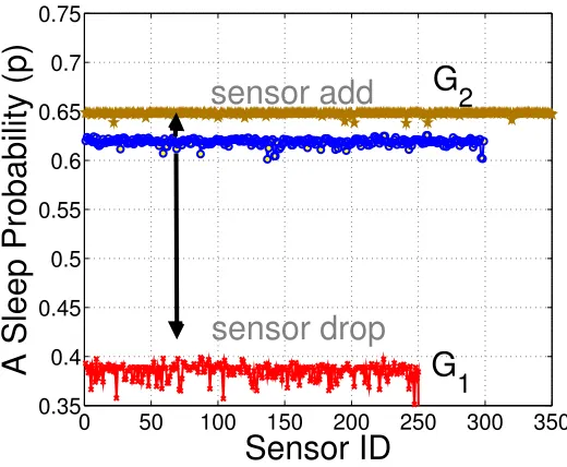
at t= 80 s (i.e., 40 s passed after the topology change. . . 21 Figure 2.6 Performance measures under sensor add/drop: G1 and G2 are graphs for
a sensor add and drop case. From the estimation of communicability and latency with varying a sleep probability p, we observe that their perfor-mance also suffers a steep degradation when the value overs the controlled sleep probability p∗. . . 22 Figure 3.1 When new technologies such as satellite and AWACS are adapted to
mo-bile opportunistic networks, it certainly helps to propagate a more recent content for mobile users. However, a still challenging question is the degree of improvement from the technology use. . . 25 Figure 3.2 Age-sensitive content propagation example: Set timest0 tot4, wheret0<
t1 < . . . < t4 and S, D and R are a source, a destination and the first
relay node that meets the destination, respectively. We stress that this dissemination is different from epidemic propagation. For example, the content C(t0) is never transmitted to D (i.e., dropped) in age-sensitive
update process. . . 28 Figure 3.3 User update rules: We make user differentiation. For D1 defined users,
they utilize only opportunistic contacts for updates. On the other hand, D2 users are capable to access an infrastructure and proceed the
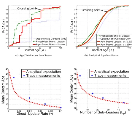
Figure 3.4 Numerical results: In sub-figs (a),(c) and (d), they respectively show the freshness comparison (i.e., quantified enhancements) of rules S2, S4
and S5, compared to S1.Sub-figure (b) plots the trade-offs between S2
(threshold-based) and S3 (age-based). . . 38
Figure 3.5 Trace results: Sub-fig (a) and (b) show the CDF of content-age distribu-tion underS1 ∼S3with parametersγ = 0.005, (γ1, γ2, τ) = (0.003,0.0077,50),
λ= 0.0957 andN = 62. (c) and (d) are mean-age comparisons when up-date rules S2 and S5 are used, respectively, with λ= 0.0957 andN = 62. 42
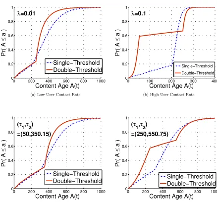
Figure 4.1 We study the performance of (a) content update process, which measures the efficiency of time-sensitive content propagations in MANETs. Espe-cially, we measure the process efficiency when mobile devices utilize (b) the sleep/awake rules for energy-saving. . . 48 Figure 4.2 Analytical CDFs for content age distribution: (a) and (b) plot the
per-formance difference of S1 and S2 depending on mobile contact rate λ variations. (c) and (d) show differences on age distribution for different en-ergy normalization tuples. Network parameters are set as (γ, τ∗, τ1∗, τ2∗) = (0.001,200,50,250.1). . . 58 Figure 4.3 Roller-net trace results: (a) shows the age distribution of users without a
device sleep/awake. (b) and (c) plot age distributions with sleep/awake rules, where τ∗= 300 and (τ1∗, τ2∗) = (100,447.36), and analytical CDFs, respectively. (d) plots the device energy consumption in t∈(0,9976]. . . . 60 Figure 4.4 (a) plots the energy consumption ratio for several energy normalized
(τ1, τ2) tuples whenτ∗= 300. (b) Mean content age supports simple
per-formance comparisons between different energy-saving rules with values. . 62
Figure 5.1 The necessity of multi-path consideration: (a) Incoming data selects one neighbor which is on the shortest path. (b) An incoming power flow is distributed into all neighbors depending on potential differences. . . 66 Figure 5.2 Whennedges exist and each resistance is 1, an effective resistanceReisn
and 1n for a path and a parallel graph, respectively. This computation in-cludes all-possible paths between A andB under potential differences. We useReon general graphs as a distance metric to measure the vulnerability
of smart-grid networks. . . 68 Figure 5.3 (a)-(b) are local degree CCDFs (Semi-Log) in IEEE 118 Bus. (c)-(d) plot
kirk graphs after threshold-based filtering with varying τ. This shows asymmetric edge removal behaviors under the use of metric S1. . . 74
Figure 5.4 Normalized centrality comparisons between closeness metric (CC) and
proposed metric S2 for (a) IEEE 118 and (b) IEEE 300 bus power grids. . 76
Figure 6.1 Electric generators convert mechanical power to electrical power. Regard-less of generation source (e.g., fuel, solar, wind and etc), its operation is based on turbine rotations and the conversion can be expressed as non-linear equations. Eq (7.1) shows a swing equation, the simplest 2nd order case. . . 82 Figure 6.2 7 bus power grid with one algebraic node: Elimination of the algebraic bus
7 by using (6.6) induces a complete admittance graph among generators. . 86 Figure 6.3 The spectral property conservation: Eigenvalues of G1 can be equal or
only have a small error even under the simpler graph G2. . . 89
Figure 6.4 System mode comparisons between a PSAT Simulation and a reduced power system model when generator 5 is a reference in IEEE 14 BUS system . . . 93 Figure 6.5 A structural sparsification of IEEE 30 BUS: The reduced graph (b) and
(c) preserve the spectral graph properties of (a) with less edges. . . 95 Figure 6.6 Eigenvalue comparison results and error-bound ǫ for several electricity
grid test-beds after the sparsification of Lby using Alg. 2. . . 96 Figure 6.7 An error-bound control capability test in 50 machine system: We measure
the error-bound with varying a sampling number (q). In Alg.1 [98], an error-bound is controlled by |E′|=O(nlogn/ǫ2) and|E′| ≤q. . . 98 Figure 6.8 Eigenvalue comparison results of several electricity grids for stability
anal-ysis between an original Asys and its sparsification by using Alg. 2. . . . 99 Figure 7.1 PEV charging station and Location Service: Currently, the location of
charging stations is accessible through web applications [7]. Based on the service, the operational framework we suggest not only provides econom-ical benefits to customers, but also improves the throughput of stations and QoS offered to customers at the same time. . . 103 Figure 7.2 Charging event occurrence CCDFs in Semi-Log scale: We extract the
estimated time to reach a driving distancexfrom Taxi GPS traces, where x={100,200,400} mile. . . 107 Figure 7.3 Station Framework: We modelncharging stations as multi M/M/1 queue
system. When station services are regulated by support scheduling, we consider the decision problem of PEVs which maximizes their benefits. . . 108 Figure 7.4 The effect of optimal allocation: For t∈(0,500], (a) and (b) express the
dynamics of the number of vehicles waiting in the three charging stations. 110 Figure 7.5 The effect of size-based AQM under optimal allocation: For t ∈(0,800],
(a) and (b) show the station size dynamics under optimal allocation policy (7.6) only and Alg. 3 which considers L, respectively. . . 112 Figure 7.6 The price sensitivity functionf: When this is known to charging stations
and satisfies an one-to-one correspondence, the direct price matching to induce a desired customer behavior is available by using an inverse func-tion f−1. We consider two sensitivity types for our tests. . . 115 Figure 7.7 Station size dynamics comparison between Alg. 3 and price method 1
Figure 7.8 The station size variation with/without AQM when the price method 1 and concave f2 are used: The tick size of Y-axis is 20 in (a) and (b). . . . 119
Figure 7.9 Price method 2 test results: In all results, the customer behavior function f1 and f2 are unknown to stations. (a) and (b) plot the dynamics under
the linear f1. (c) and (d) are dynamics under the concave f2. Two price
sensitivity functions are shown in Fig. 7.6 and the parameter γ in (7.11) is set to 0.5. . . 122 Figure 7.10 The effect of regression parameter γ in method 2 price dynamics. . . 124 Figure 7.11 Test results under electric support regulations: During a day-time the
service at charging stations is regulated by (a) and eq. (7.13). (d) plots the station dynamics without price control methods. We compare the result with the dynamics under method 1 ((b) and (c)) and method 2 ((e) and (f)). . . 125 Figure 7.12 The location of commercial PEV charging stations [7]: By demands, their
installations are more likely to be clustered, than uniform. . . 127 Figure 7.13 Framework performance test under clustering: The aggregated bar graphs
notify the charging station throughput under two clustering, shown in Fig. 7.12, for 5 hours and we observe a gradual performance decrease according to clustering, compared with non-clustering (dotted line). Star notations (⋆) indicate a measured throughput after a service rescheduling, given by (7.15). . . 128 Figure 7.14 For a clustered operation of our framework, combining a Vehicle-to-Grid
(V2G) support or battery replacement stations can make atonement for the solution infeasibility of electricity scheduling that comes from service rate control constraints. . . 130 Figure 7.15 (a) shows that a PEV price sensitivity function can have a general
de-creasing shape depending on spatial- and temporal cluster differences and utilizing the differences (Alg. 4) improves the price convergence speed. . . 134
Chapter 1
Introduction
Revealing the relationship among objects is the fundamental purpose of network research. We observe that its applicable scope is not just limited in engineering areas, but spans all surrounding phenomena. Without considering the common network studies in engineering such as Internet, computer architecture, electric circuit and etc, our society itself is a kind of large-scale networks. Nowadays, it becomes more and more challenging to fulfil the fundamental goal. In many network categories, they either (both) tend to have complex inter-connections or (and) include large-scale objects. Hence, their relationships and overall network performance are not intuitive and sometimes contradictory to our anticipation. For this reason, the importance of network research should be magnified. Although my research interest spans all around network related problems, this dissertation involves performance estimation methods and reliability improvement algorithms especially in wireless sensor, mobile opportunistic networks and smart-grids.
1.1
Motivation and Overview
Network Connectivity
Wireless Sensor Networks
Mobile Opportunistic
Networks
Smart-Grids
Figure 1.1: The contents in this dissertation
that a desirable network analysis only can be obtained when we utilize methods which correctly capture the network property. In this manner, this dissertation categorizes wireless sensor and mobile networks as one, and smart-grids (more specifically power network systems) as the other, and shows that the induced network analysis can be very different when network characteristics are improperly considered. The following subsections may be helpful to understand the big picture of this subject.
balance the mentioned trade-off and also endure the time-varying connectivity issue at the same time. The combined use of percolation theory and consensus algorithm helps designing an autonomous and distributed algorithm to achieve above purposes.
1.1.2 Mobile Opportunistic Networks: Realistic Version of Delay Tolerant Networks (DTNs)
In Mobile Ad-hoc Networks (MANETs), contact patterns among users or devices have been regarded as the key element to determine the performance of data propagation. This is because data forwarding chances are temporarily allowed only when users are positioned within their communication range. In my understanding, this MANET research direction still clings to the network condition where no infrastructure is given. However, in most times, we are surrounded by centralized wide-area networks such as 3G and 4G cellular networks and utilize them for communications. Hence, the more required point now is the analysis of content propagation in MANETs under the co-existence of such infrastructure aids. Especially, popular contents in cellular data communication are more likely to be time-sensitive. For example, news headline, famous tweet or local traffic information. Customers prefer to obtain more recent contents. My focus is to determine the propagation performance of age-sensitive contents.
1.1.3 Smart-Grids : Convergence Solutions between Power and Data Net-works
1.2
Contributions and Accomplishments
1.2.1 Contributions
This subject has the following contributions in engineering society:
1. Sensor Control Algorithm: For WSNs, provide an autonomous and distributed balancing algorithm between connectivity and energy consumption of wireless sensors with preserv-ing an algorithm simplicity. This not only brpreserv-ings a cost reduction for network construction, but also reduces the burden of sensor management.
2. Stochastic Modeling and Validation: For mobile opportunistic networks, propose a stochas-tic modeling approach to determine the performance of age-sensitive content propagation also with validations through real traces. The modeling can be applicable not only for de-lay tolerant network analysis, but also several hybrid network cases such as the existence of infrastructure aids or the deployment of device energy-saving strategies.
3. Power Grid Vulnerability Analysis: For smart-grids, suggest performance metrics to mea-sure network vulnerabilities of power grids with considering electric properties. This gives a lesson such that topology-based power grid analysis is insufficient and reveals one rea-soning of cascading failure phenomena in power grids.
4. Complexity Reduction Methods: In power systems, mathematically tractable method, so called small-signal stability analysis, is not applicable to current power system trends due to high complexity. This subject supports the simplification of electric generator dynamic analysis and the suggested technique gets more benefits with system size increase. 5. Information System with High Abstraction: For the proliferation of PEV (Plug-in Electric
Vehicle), design a charging station framework which improves customer QoS (Quality of Service) and station throughput at the same time. Several performance-related parame-ters such as expected waiting time of customers, station congestion and electric support scheduling are integrated into price mechanisms and this lets customers get benefits with ease.
1.2.2 Accomplishments
Above contributions are printed on the following publications and some parts of this dissertation include reprints of them:
Daehyun Ban, George Michailidis, and Michael Devetsikiotis, “Price Based Mechanisms for PEV Charging Stations with Spatio-Temporal Difference Awareness”, submitted to IEEE Transaction on Smart Grid.
Daehyun Ban, George Michailidis, and Michael Devetsikiotis, “Demand Response Control
for PHEV Charging Stations by Dynamic Price Adjustment”, IEEE Innovative
Smart-Grid Technology (ISGT), 2012.
Daehyun Ban, George Michailidis, and Michael Devetsikiotis, “Towards Improved Scal-ability in Smart Grid Modeling: Simplifying Generator Dynamics Analysis via Spectral
Graph Sparsification”, IEEE SmartGridComm; Modeling and Simulation, 2011.
Daehyun Ban, and Michael Devetsikiotis, “Content-Freshness Enhancements with
Infras-tructures in Mobile Opportunistic Networks”, IEEE Military Communication (MILCOM),
2011.
Daehyun Ban and Michael Devetsikiotis, “Flow-Based Centrality Measure through
Resis-tance DisResis-tances in Smart-Grid Networks”, IEEE Global Telecommunication
(GLOBE-COM), 2011.
Daehyun Ban and Michael Devetsikiotis, “Content-Update Process Performance under
Energy-Saving Schemes in Mobile Opportunistic Networks”, IEEE Latin-America
Com-munication Conference (LATINCOM), 2011.
The co-author Dr. Michael Devetsikiotis listed in these publications directed and supervised the research which forms the basis for the dissertation.
1.3
Road-Map of This Dissertation
The road-map of this dissertation is broadly divided into two parts: In part I, from chapter 2 to 4, each chapter provides either data network analysis methods or algorithms based on connectivity-pattern. Chapter 2 discusses about an autonomous performance balancing between a time-varying network connection topology and the energy consumption of wireless sensors in static networks. Chapter 3 visits the performance analysis in mobile opportunistic networks with the co-existence aid of infrastructures. The modeling approach, used in chapter 3, is revisited in chapter 4 to analyze the energy-saving effect of mobile devices.
Chapter 2
Balancing Network Connectivity
and Life-Time of Wireless Sensors
through Percolation and Consensus
2.1
Chapter Abstract
Due to replacement infeasibility, methods to extend the life-time of sensors have been an issue in Wireless Sensor Networks (WSNs) and these should consider network connectivity simul-taneously. At this point, controlling the sleep/awake of sensors is one simple way to reduce their energy consumption. However, this causes a network connectivity degradation by vary-ing network connection topology. For this reason, we propose a simple and autonomous sensor sleep/awake method to achieve their balance.
information becomes challenging under physical topology changes such as sensor add/drop. We show that the global knowledge requirement can be resolved by using a consensus algorithm. Through several graph tests, we show that our method achieves a network balancing between connectivity and life-time with preserving its simplicity. Also, the balancing is autonomous even under physical topology variations.
2.2
Chapter Introduction
As the tool of network construction, the primary purpose of wireless sensors is on the estab-lishment of network connectivity. In contrast to other devices with an external energy support, they are generally operated by battery power which causes the periodic replacement of en-ergy source. Moreover, their installed locations are uncoordinated in many network scenarios and this makes the replacement harder due to uncertain sensor locations. In this respect, we observe that methods to extend network life-time by the energy-saving of sensors receive at-tentions in [25, 96, 102, 44, 49, 106, 76, 19]. In the procedure, it is also required to consider network connectivity with them.
shortest-path finding on dynamic graphs. However, for a sophisticated network management, these go through a reinforcement period with heavy computational burdens. We can additionally observe a multi-path routing for the balanced energy consumption of sensors [76] and the use of mobile sensors for data aggregation [19]. Still, these require either global topology information or a time synchronization among sensors. From these observations, we need to reconsider whether sensors can percept the global information and endure the computational complexity.
The necessity ofsimpleandefficientenergy-saving methods is not invariant to sensor deploy-ment conditions. We frequently observe situations when the sensor deploydeploy-ment is uncoordinated (e.g., military operations which need a rapid infrastructure construction or data collection net-works under extreme weather conditions). This restricts the use of above mentioned schemes in that sensors do not know the global topology information. Also, we need to concern the cost for purchasing sensors. Using non-expensive sensors limits to execute complex algorithms due to sensor processing capability. For these reasons, this chapter proposes a simple and distributed energy-saving method which resolves above issues.
Percolation theory is widely used to determine clustering behaviors on graphs [92]. Espe-cially, it reveals that the appearance of giant clusters has a phase transition behavior depending on edge connection patterns [32, 23]. We observe that this transition behavior can be related to an energy-saving algorithm if sensors know their global connection topology [41] and the restriction is partly relaxed by utilizing local edge degrees in [67]. In contrast to them, we sug-gest a distributed method to obtain the global information by using a consensus algorithm and show its effectiveness in balancing network qualities between connectivity and energy-savings.
2.3
Problem Description
2.3.1 Network Conditions and Assumptions
We consider a WSN withnstatic sensors and define a graphG which represents its connection topology. While constructing the network, the sensor deployment is uncoordinated. Therefore, the topology is unknown information for sensors.
Each sensor makes an independent sleep/awake decision to extend its life-time. In a discrete-time system, we set a parameter p which implies the sleep probability of sensors and consider that a sensor energy consumption is proportional to its awake period. Under these, the connec-tion topology is time-varying and the topology graphG is dynamic (i.e.,G(t)).
Due to cost limitation, we assume non-expensive sensors whose functionalities are restricted. Computations are eligible only for light loads due to small memory space. Also, they do not have a power control (i.e., only have an on/off option) and a time synchronization scheme with other sensors.
In the circumstance, the sleep probability p is an important parameter which decides the network performance. We want to find a value which balances the network connectivity and the energy-consumption of sensors. Additionally, the value needs to be adjusted autonomously even if there occur physical topology changes such as sensor add/drop (e.g., additional sensor installations after the first deployment or imbalanced sensor die-outs due to unfair energy consumptions).
2.3.2 Performance Measurement Metrics
We use two metrics to estimate network performance and these are based on packet transmission conditions. Each sensor periodically generates a packet whose destination is uniform randomly selected among n−1 other sensors. For those packets, we consider the following metrics (Note. the only distinction is whether a delayed packet delivery is allowed or not):
observe whether there exists a path to its destination under the connection topology
G(tk). If the topology does not have a path, the packet is dropped. This metric measures
the rate of successful path existence at each packet generation instance.
Latency: In contrast to Communicability, a packet is not dropped under no path
exis-tence. Instead, it waits until the first path is established on the time-varyingG(t) and we observe the delay for each packet. Latency measures the mean delay of packet transmis-sions.
Additionally, we estimate the average sleep probability of sensors during tests to measure the degree of energy-saving. When the value is ¯p, this implies that network sensors save their energy consumption with degree ¯p.
2.4
Controlling the Sleep/Awake of Sensors with Percolation
Theory and Consensus Algorithm
We explain the reason how the giant-cluster condition in percolation theory matches to the sleep/awake control in WSNs. From there, we observe the necessity of global topology informa-tion. By adding an average consensus algorithm on it, we propose a sensor sleep/awake method to balance network qualities between connectivity and energy-consumption.
2.4.1 Matching Giant-Cluster Condition to Sensor Sleep/Awake
Percolation theory investigates the behavior of clusters on graphs and one attractive result is the sharp transition of cluster size according to edge connection patterns [32, 23]:
Theorem 1 (The Phase-Transition of Cluster-Size [32])A graph G has a giant-cluster
with high probability if each node has connections with at least two other nodes. When a random
Ψ(G) = E[X
2]
E[X] ≥2 (2.1)
Because of a path existence among any cluster node, measuring the size can be useful to estimate the network connectivity degree. When we utilize a sensor on/off algorithm, suppose that a sensor makes a sleep decision at timetkin the network. This decision simply corresponds
to the node removal on a time-varying connectivity graph G(tk). For this reason, finding out
the feasible fraction of random node removal on G which satisfies Theorem 1 is equivalent to the region of statistical sensor sleep probabilitypthat prevents a severe connectivity loss in the network.
For the graph with p fraction node removals, [32, 23] show procedures to gain the first and second moments of edge degree distribution. When we set E[X0] and E[X02] as the two
moments of G, respectively, and combine them with (2.1), it gives the feasible range of sensor sleep probability, which conserves the giant-cluster condition, as follows:
p≤1− E[X0]
E[X2
0]−E[X0]
(2.2)
In WSNs, we observe that similar approaches are used in [41, 67]. However, in there, the global information (i.e., the first and second moments) is stillunknown for local sensors when their deployment is uncoordinated.
2.4.2 Consensus Algorithm
In multi-agent systems, consensus algorithms define methods to reach a value agreement among agents only with local interactions (see the survey [82] and references therein for details). Especially, the sleep/awake formulation (2.2) lets us focus on an average consensus. Even for a dynamic graph G(t), we observe that there exist algorithms that achieve a value convergence and choose such an algorithm from [83].
Under this dynamic graph, each node proceeds the following distributed simple decision:
˙ xi(t) =
X
j∈Ni(t)
(xj(t)−xi(t)) (2.3)
wherei= 1,2, . . . , nandNi(t) is ai’s neighbor set at timet. This leads an asymptotic value convergence given by:
x1(t) =x2(t) =. . .=xn(t) =α (Average Consensus)
We note that the sum of all node states (i.e., Pix˙i) is invariant to time. This implies that
the sum of initial valuesPi∈V xi(0) is preserved regardless of time. For all agents, (2.3) always
leads a direction where the value gap with neighbors decreases. These support that the value agreement α reaches n1 Pi∈V xi(0) (i.e., an average consensus) in steady-state.
2.4.3 Sleep/Awake Control for Performance Balancing
In our method suggestion, each sensor only requires four values and a simple computing ca-pability. For sensor i, we set parameters xi1,xi2,xTi1 and xTi2. First two parameters decide the
sleep/awake probability pand the other two are used to reflect physical topology variations.
Initial Value Estimation
The essence of the average consensus is on the equal distribution of the initial value sum
P
i∈V xi(0) through linear interactions. Hence, an initial value estimation is important to reach
a correct value agreement.
Each sensor is required to measure its local edge degree when all sensors are awake. Suppose thatGois the connection topology. For sensors, estimating the local degree is not instant as they are utilizing an independent sleep/awake. Hence, they first have a waiting phase to measure an exact local degree.
⌈1−1ξ⌉ slots, where ξ is reasonably close to 1. Each sensor uses this local measurement and its
square value as xi1(0) andxi2(0), respectively, and joins the following consensus process.
Consensus Process and Sleep Probability Decision
Sensors proceed two consensus processes with local neighbors, given by:
˙
xi1(t) =Pj∈Ni(t)β(xj1(t)−xi1(t)) ˙
xi2(t) =Pj∈Ni(t)β(xj2(t)−xi2(t))
(2.4)
where i, j ∈ V and Ni(t) is a neighbor set at time t. β is a small positive constant and affects the speed of convergence.
From [83], these processes are guaranteed to reach an average consensus even if the con-nection topology is dynamic. Hence, in steady-state, sensors have the global informationE[X0]
and E[X02] in (2.2). During the consensus processes, we utilize transient measurements xi1(t)
and xi2(t) to set up a sensor sleep probability pas follows:
pi(t) = 1−
xi1(t)
xi2(t)−xi1(t) −
ψ (2.5)
We are aware that this sleep probability decision also arrives at a consensus among sensors as the two independent processes guarantee a convergence. When ψ= 0, the sleep probability p locates on the phase-transition boundary in (2.1). For this reason, we set a small positive constant ψ to prevent a steep connectivity loss.
Sleep Probability Adjustment for Topology Variations
During a network operation, the life-time of sensors is uneven. Moreover, we can install addi-tional sensors. These make the connection topology graph G sparser or denser. In these cases, sensors are required to find a newly balanced sleep probability p for the varied topology. By using the average consensus, an autonomous sleep probability adjustment is capable.
sensors to detect their local degree variation when there occurs an add/drop. Then, the issue is how effectively reflect the local topology change into the consensus process for global parameter estimations.
Once after a sensor participates in the consensus process (2.4), its parameters xi1 and xi2
keep varying to the convergence valuesE[X0] and E[X02], respectively. Hence, substituting the
newly measured local degree and its square values intoxi1 and xi2 during the process does not
make correct convergence values for the varied topology.
The property of selected consensus algorithm is the equal distribution of total state sums
P
i∈V xi1 andPi∈V xi2. For this reason, fitting those values according to the topology variation
is one way to reach a correct consensus. We suggest a simple recursion by using parametersxT i1
andxTi2. When sensors join the consensus process, their parametersxi1 and xi2 are same asxTi1
and xTi2, respectively. Then, suppose that a sensor i acknowledges that its degree is changed at t and the value isxnewi . By using dummy parameters xTi1 and xTi2, we consider the following recursions:
xi1(t+) =xi1(t) +δ1, xi2(t+) =xi2(t) +δ2 (2.6)
where δ1=xnewi −xTi1 and δ2= (xnewi )2−xTi2. After the changes, the sensor puts xnewi and its
square value into xT
i1 and xTi2, respectively.
These recursions reflect the number of added (or subtracted) edges when a topology change occurs and lead the consensus algorithm to be aware of the correct total edge degree sum during operations.
2.5
Simulations on Random Graphs
1 2 3 4 5 6 7 8 9 10 11 12 13 14 15 16 17 18 19 20 21 22 23 24 25 26 27 28 29 30 31 32 33 34 35 36 37 38 39 40 41 42 43 44 45 46 47 48 49 50 51 52 53 54 55 56 57 58 59 60 61 62 63 64 65 66 67 68 69 70 71 72 73 74 75 76 77 78 79 80 81 82 83 84 85 86 87 88 89 90 91 92 93 94 95 96 97 98 99 100 101 102 103 104 105 106 107 108 109 110 111 112 113 114 115 116 117 118 119 120 121 122 123 124 125 126 127 128 129 130 131 132 133 134 135 136 137 138 139 140 141 142 143 144 145 146 147 148 149 150 1 2 3 4 5 6 7 8 9 10 11 12 13 14 15 16 17 18 19 20 21 22 23 24 25 26 27 28 29 30 31 32 33 34 35 36 37 38 39 40 41 42 43 44 45 46 47 48 49 50 51 52 53 54 55 56 57 58 59 60 61 62 63 64 65 66 67 68 69 70 71 72 73 74 75 76 77 78 79 80 81 82 83 84 85 86 87 88 89 90 91 92 93 94 95 96 97 98 99 100 101 102 103 104 105 106 107 108 109 110 111 112 113 114 115 116 117 118 119 120 121 122 123 124 125 126 127 128 129 130 131 132 133 134 135 136 137 138 139 140 141 142 143 144 145 146 147 148 149 150
(a) Ψ(G) = 2.0482 (b) Ψ(G) = 1.9200
Figure 2.1: We generate two random graphs whose Ψ is slightly over and less 2 with 150 nodes and observe a steep decrease on their maximum cluster size.
2.5.1 Cluster Size Variation and Average Consensus
Our sensor sleep/awake method arises from the correctness of the giant-cluster condition and average consensus algorithm. For this reason, we provide simple results to recognize their va-lidity.
Phase-transition on the cluster size
Theorem 1 implies that the cluster size on random graphs suffers a shape transition around Ψ = 2. In Fig. 2.1, we plot two random graphs with 150 sensors. By varying the edge construction probabilitye, their Ψ is controlled to be slightly over (2.0482) and less (1.92) than 2, respectively. We estimate their maximum cluster size and observe the occurrence of a steep size reduction (51→14) around Ψ = 2. Except the case, we observe that the cluster size reduction is gradual with the Ψ decrease (similar results are observed in [91]).
Average consensus on dynamic graphs
0 200 400 600 800 1000 0 2 4 6 8 10 12 Time
Number of Neighbors
Convergence to an average
0 200 400 600 800 1000 0 2 4 6 8 10 12 Time
Number of Neighbors
Convergence does not occur
0 200 400 600 800 1000 0 2 4 6 8 10 12 Time
Number of Neighbors
Convergence to an average
(a) Under an original topology (b) One time random reduction (c) Renewal of random reduction on (b)
Figure 2.2: Convergence test of consensus algorithm: For tests, we generate a connected random graph with 300 nodes whose average edge degree is 3.184, and apply static and dynamic node sleep/awake strategies. These show that the consensus algorithm on (2.3) reaches a convergence into the average even under dynamic node removals.
of sensors under the topologyG and its dynamic node removal withp= 0.4 which corresponds to a sensor sleep/awake scenario, respectively. For both cases, they show a convergence into the correct average and the only difference appears as the speed of convergence. This verifies that (2.3) can be utilized to find a balanced sleep probability punder sensor sleep/awake scenarios.
2.5.2 The Proposed Sensor Sleep/Awake Method Tests
By using Communicability and Latency, we test the performance of proposed sleep/awake method. These metrics are designed to measure network connectivity through packet trans-missions. We are aware of the steep transition of cluster size and its occurrence is highly related to the sensor sleep/awake decision. This allows us to expect that the similar performance tran-sitions will appear on communicability and latency measurements.
No Sensor Add/Drop Case
0 50 100 150 200 250 300 0.4
0.45 0.5 0.55 0.6 0.65 0.7 0.75
Sensor ID
A Sleep Probability (p)
0 50 100 150 200 250 300 0.4
0.45 0.5 0.55 0.6 0.65 0.7 0.75
Sensor ID
A Sleep Probability (p)
(a) Sensor sleep probability att= 10 s (b) Sensor sleep probability att= 40 s
Figure 2.3: We observe the sleep probability of sensors att= 10 and 40 s. Att= 40, the sleep probability reaches an agreement among 300 sensors to the expected valuep= 0.619.
probability pof sensors is 0.619 when a convergence occurs by using (2.4) withψ= 0.04. First, we test whether our method leads the expected p. At initial, we set p= 0.5 for all sensors. Fig. 2.3 plots two snapshots for the sleep probability of 300 sensors. At t= 10 s, we observe a sleep probability disagreement among sensors. The difference diminishes by using (2.4) and (2.5). At t= 40 s, the sleep probability snapshot almost shows an agreement with the expectedp. This can be a validation that two independent consensus processes in (2.4) also reach a correct convergence.
By measuring communicability and latency, we investigate the effectiveness of the controlled sleep probability. We assume that sensor generate a packet at every second with a uniform des-tination. In Fig. 2.4, we plot the two metric results with varying the sleep probability of sensors. For communicability, it generally decreases with the increase of sleep probability. However, one notable point is the decreasing degree of measurements. We see that communicability shows a steep decrease when the sleep probability of sensors is over the controlled pvalue. This nature is similarly observed in the latency measure with having a sharper transition behavior.
perfor-0.2 0.4 0.6 0.8 0
0.2 0.4 0.6 0.8 1
Sleep Probability (p)
Communicability (rate)
Consensus Value p = 0.618
0.2 0.4 0.6 0.8
0 10 20 30 40 50 60 70
Sleep Probability (p)
Latency (Sec)
Consensus Value p = 0.618
(a) Communicability (b) Latency
Figure 2.4: Performance measures under no sensor add/drop: We plot communicability and latency with varying a sleep probabilitypand observe the steep performance degradation when sensors set their p over the controlled valuep∗.
mance. For example, from the latency measure Fig. 2.4(b), it allows sensors to save 60% energy consumption only with a slight delay increase in packet transmissions.
Sensor Add/Drop Case
While operating a WSN, the additional installation or uneven die-out of sensors can make changes onG. We test whether the proposed method can autonomously adjust the sleep prob-ability p under those cases.
For consistency, we start from the graph G in the previous. In there, sensors reach a sleep probability consensus at 40 s withp= 0.619. We uniform randomly drop and add 50 sensors onG at 40 s and define their graphs asG1andG2, respectively. The followings are their measurements
whereG(# of sensors,Ψ, E[X0], E[X02], Expected p):
G1(250,3.06,1.71,4.61,0.38), G2(350,6.19,3.17,12.88,0.64)
0 50 100 150 200 250 300 350 0.35
0.4 0.45 0.5 0.55 0.6 0.65 0.7 0.75
Sensor ID
A Sleep Probability (p)
sensor add
G
1
G
2
sensor drop
Figure 2.5: The sleep probability of sensors forG1 (sensor add) andG2 (sensor drop) att= 80
s (i.e., 40 s passed after the topology change.
is also increase (decrease). In Fig. 2.5, we plot the sleep probability of sensors at 80 s. For both add and drop cases, we see that preaches another agreement value that exactly corresponds to our analytical expectation. We note that sensors reflect the topology variation locally by using (2.6) and the value adjustment is achieved only by distributed local interactions.
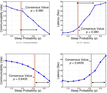
In Fig. 2.6, we measure communicability and latency with varying the sleep probability p forG1 andG2. In there, we observe that the metric performance decreases with the increment of
p. Especially, there still exists the region where steep performance declines occur. We indicate the controlled sleep probability p, which is attained by using the proposed method. For both communicability and latency, those values locate just before the steep performance reduction.
In Fig. 2.6(a), the controlled p saves 38% energy consumptions with less than 10% com-municability reduction. Also, Fig. 2.6(d) indicates that almost 65% energy can be saved only with a 5 s delay increase. It is extremely notable that utilizing a consensus algorithm gives an
autonomous property to find out the balanced peven under topology variations.
0.2 0.4 0.6 0.8 0.1 0.2 0.3 0.4 0.5 0.6 0.7 0.8
Sleep Probability (p)
Communicability (rate)
Consensus Value p = 0.380
0.2 0.4 0.6 0.8
5 10 15 20 25 30 35 40
Sleep Probability (p)
Latency (Sec)
Consensus Value p = 0.380
(a)G1 communicability (b)G1latency
0.2 0.4 0.6 0.8
0 0.2 0.4 0.6 0.8 1
Sleep Probability (p)
Communicability (rate)
Consensus Value p = 0.6435
0.2 0.4 0.6 0.8
5 10 15 20 25 30 35
Sleep Probability (p)
Latency (Sec)
Consensus Value p = 0.6435
(c)G2 communicability (d)G2latency
Figure 2.6: Performance measures under sensor add/drop: G1 and G2 are graphs for a sensor
sensors. The sleep probability of sensors reaches an agreement in steady-state and the duration to reach the state appears as a relatively short period in our tests. Under the assumption that sensors consume an energy only when they are awake, this additionally resolves the imbalanced energy consumption of sensors, dealt in [76].
2.6
Chapter Summary
In WSNs, the life-time extension of sensors is required due to their replacement infeasibility and the method must be proceeded under the network connectivity assurance. Controlling the sleep/awake of sensors is one way to extend the life-time. However, it has a trade-off against network connectivity and is challenging to find out their balanced point.
Chapter 3
Age-Sensitive Content
Dissemination with Infrastructures
in Mobile Opportunistic Networks
3.1
Chapter Abstract
Chapter 3 investigates the effect of infrastructures in mobile opportunistic networks. Due to the absence of guaranteed connectivity, opportunistic networks have put emphasis on mobile contact information to investigate their performance. But, mobile users (e.g., smart-phone cus-tomers) generally live under wide-area networks such as 3G/4G communication systems and this implies that they are able to access a desired content almost without spatial and temporal limitations. For this reason, we determine the improvement degree of content propagation when opportunistic users access an infrastructure to update the content with having several rules.
content update process when opportunistic contacts occur.
Figure 3.1: When new technologies such as satellite and AWACS are adapted to mobile op-portunistic networks, it certainly helps to propagate a more recent content for mobile users. However, a still challenging question is the degree of improvement from the technology use.
In addition to this update process, we propose several infrastructure access rules for mobile users. Then, the network performance varies according to the rule and content update process, and we quantify the degree of performance changes in age-sensitive content dissemination. For wide-area access technology, this chapter consider a scenario when satellite or AWACS are utilized in battle-field.
The analysis is based on stochastic ODE modeling. We analyze the content freshness changes for each update rule when users have a poisson contact and compare the performance between different rules. In addition, those suggested rules are tested on real contact traces. We validate our analytical solution from the comparison with analytical solutions.
3.2
Chapter Introduction
appli-cations for military purposes and sensor devices are frequently used to construct a temporary network [71, 112, 51]. Sensors can build a mesh network by static installations and they also support a Delay Tolerant Network (DTN) as mobile relays [68].
For the purpose of content updates, we consider a network where sensors are utilized as mobile relays. In there, an information provider keeps renewing atime-sensitive content, while mobile users update the content by depending on opportunistic contacts. A time-sensitive con-tent means that its information freshness decreases with time (e.g., news, traffic information or commands in military operation). Mobile users preserve the more recently generated content between encounters in that they prefer up-to-date information for the content. This contact-based update may not be suitable for the delivery of time-sensitive contents, as users suffer a large delay for an update when the contact rate is low.
The emergence of new communication technologies can relax this problem. For example, in a military operation, a satellite or an Airborne Warning and Control System (AWACS) is deployed in operation areas. They can provide a temporary communication infrastructure in a short time as shown in Fig.3.1. In this chapter, we are interested in the enhancement of content update process when the infrastructures are added to a contact-based network.
It is crucial to quantify the effectiveness of new technologies. In mobile opportunistic net-works, [15] analyzes the reduction degree of packet transmission delay by installing base-stations and relays. Also, for databases, [30, 74] show the improvement of data consistency under the use of several cache update schemes.
utilize the concept ofcontent-age which is used in [26, 11, 56]. We model the freshness changes according to the use of different update rules and quantify the freshness improvement that users receive.
The remainder of this chapter is as follows: In section 2, we explain the difference between our update process and the approach in [15]. Then, we formulate an update problem under the existence of an infrastructure. Section 3 provides the reasoning for our modeling and shows the freshness variation under each update rule.
We also provide numerical comparisons among suggested rules. In section 4, our update rules are tested on real-traces and we compare the result to our analytical expectations. After that, we conclude this chapter.
3.3
Background and Problem Formulation
By using the example of epidemic content propagation, we clarify the difference of our update process from [15]. After that, we define “content freshness” and “update process” and formulate our content update problem with an infrastructure in mobile opportunistic networks.
3.3.1 Multi-Packet Delivery in Epidemic Routing
In DTNs, connectivity among network users is not always guaranteed. To overcome this short-coming, each user utilizes astore andforward scheme with the role ofrelay andsink at a same time. Epidemic routing guarantees a minimum transmission delay in the network. In paper [15] which analyzes the improvement of content propagation by infrastructures, mobile users still fol-low the epidemic routing when a contact occurs. Specifically, the delay measure of it is based on an Ordinary Differential Equation (ODE) model of epidemic routing [114]. Before this, Markov Chain (MC) models have been used to estimate a packet delay in epidemic routing [48]. The ODE model comes from the fluid-limit of the MC. Under a feasible scaling, the ODE solution can substitute to solve the MC with less complexity [114, 70].
S
R
D
Figure 3.2: Age-sensitive content propagation example: Set times t0 to t4, where t0 < t1 <
. . . < t4 and S, D and R are a source, a destination and the first relay node that meets the
destination, respectively. We stress that this dissemination is different from epidemic propaga-tion. For example, the content C(t0) is never transmitted toD (i.e., dropped) in age-sensitive
update process.
model for a packet delay in epidemic routing. Suppose a network with nusers whose pair-wise meeting rate isβ and setI(t) andP(t) as the number of content holders (i.e., infected) and the delay CDF (i.e., P(t) = Pr(Td < t)), respectively. Then, an ODE model for epidemic routing
is:
I′(t) =βI(t)(N −I(t)), P′(t) =βI(t)(1−P(t)) (3.1)
With initial conditions I(0) = 1 and P(0) = 0, the closed-form solutions is:
P(t) = 1− N
N −1 +eβN t, E[Td] =
lnN
β(N −1) (3.2)
This is an analysis for a single packet transmission delay and can be extended to multi-packet cases with ease when users do not have a buffer-limit. For each packet, its propagation is
independent from others so that the induced packet delay is identical under this approach.
3.3.2 Content Update Process
content. We assume that a content is fresher if the elapsed time from a source departure is smaller and define the elapsed time as content-age, A(t). This is useful to distinguish the freshness. A source is considered to have a fresh information (i.e,A(t) = 0) all the time [26, 11, 56]. By using the content-age, a content update process to share a fresh content is described as follows:
Content update process: When a contact occurs between users, they compare their
content-age and share the lesser of the two (i.e., min{Ai(t), Aj(t)}).
In this process, contents have a dependency and users have a buffer-size limitation, as only holding an up-to-date content. During content propagation, there exists a fundamental difference as shown in Fig.3.2. Under an ascending time ordertn, we setS, Dand R as source,
destination and the first relay which delivers the content ofS toDfor the first time.S updates its content at t0 and t2. R meets S at t1, t3 and D at t4. Then, D only receives the content
C(t2) at t4. In contrast to [15],C(t1) is never propagated to Din the update process.
Hence, the approach to measure the effect of infrastructure in [15] has different propagation dynamics from our update process. Moreover, the focus of our update process is on the change of content freshness through user interactions.
3.3.3 Content Update Problem with Infrastructures
We start from considering a military operation in a region without infrastructures. There is a
Direct-Update
We additionally consider the deployment of satellite or AWACS in the network. For users, these facilities allow the following direct-update:
Direct-update: An IP uploads its commands continuously into a satellite or an AWACS
used as an information storage. Each user is allowed to access the storage for updates, limited by user update rules. We assume that an IP and a storage is synchronized so that users receive the effect of an IP contact from direct-updates.
There can exist several reasons for limiting the direct-update (e.g., energy-consumption of devices, portability and device cost issues). We consider two device categories D1 and D2.
For updates, D1 only utilizes opportunistic contacts, whereas D2 can use both contacts and
direct-updates. In the following, we define the operation rules of the devices.
Content Update Rules for Users
For all update rules, users utilize opportunistic contacts for updates.
Opportunistic Contact Only (S1): Users utilize only mobile contacts for the update
of IP contents. This is for the performance comparison with other rules.
Probabilistic Direct-Update (S2): All users have D2 devices. To extend device
life-time, each user chooses a direct-update with rate γ.
Age-Based Direct-update (S3): Under probabilistic direct access, users can decide a
direct-update even if they have a fresh content (i.e., young age). To prevent this, users control the rate of direct-access based on their content age,A(t). There exists a threshold-age τ and the direct-access rate is set to γ1 (low rate) and γ2 (high rate) when A(t) is
lower and higher than τ, respectively.
Base-Station Update (S4): Users utilize only opportunistic contacts for updates.
with the IP are installed in a network. With an inter-contact rateχ, each user visits one of BSs and updates an age 0 content.
Sub-Leader Update (S5): With high frequency, a partial number (L2) of users chooses
a direct-update. The remaining users receive the effect of direct-updates from the contacts with those partial users.
In the following section, we show the changes of user content freshness (i.e., age) from the interaction of users and the update rule selection.
3.4
Model and Analysis
As mentioned, we utilize a content age A(t), specifically a mean content age, as a metric to compare the content freshness of users. For one user, we first observe the age dynamic of content update process. Then, we explain the reasoning of how to compute the content-age distribution of users and derive the close-form solutions from ODE modeling. They allow us to see the variation of freshness under each rule. We show numerical results and analyze the quantity of freshness improvement.
3.4.1 The Age-Dynamics of Users
We select useriat timetand describe its age variation for a smallǫtime duration, wherei∈ V. If we assume that the time consumption for updates is negligible, the age at t+ǫis:
Ai(t+ǫ) =
ǫ under condition 1
min{Ai(t), Aj(t)}+ǫ under condition 2
Ai(t) +ǫ otherwise
(3.3)
Direct-Access
User (
)
General User(
)
(a) Opportunistic Contact Only (S1)
(b) Direct-Update by All Users (S2 andS3)
(c) Direct-Update by Partial Number of Users (S4andS5)
Figure 3.3: User update rules: We make user differentiation. ForD1 defined users, they utilize
only opportunistic contacts for updates. On the other hand, D2 users are capable to access
to the update rules, the probability of condition 1 varies (e.g., an IP contact probability is
ǫλ
N). Condition 2 describes a contact between users. From the rate of inter-any-contact, the
probability becomes NN−1ǫλ. We utilize this age-dynamics to construct an ODE model for the content age distribution of users.
3.4.2 Age-distribution and Mean-Content Age
To investigate the age distribution of users, we provide an ODE model based on a mean-field regime [26, 70]. We define F(t, a) as the state of ODE, where F(t, a) ≡ P(A(t) > a). The state includes two dynamic variables (time and age). Hence, its ODE form has the following expression:
dF(t, a) dt +
dF(t, a) da = limǫ→0
F(t+ǫ, a)−F(t, a−ǫ)
ǫ (3.4)
where∓F(t, a) canceled out each other on the right-hand side. Suppose that it reaches a steady-state (i.e., t→ ∞). Then, the time dynamics can be ignored so that dFdt(t,a) = 0 and theF(t, a) is abbreviated toF(a) which is the Complementary Cumulative Distribution Function (CCDF). Under this case, eq. (3.4) provides an ODE for the content age-distribution of a user in steady-state.
By choosing one user i and using the age dynamics (3.3), we compute Fi(t+ǫ, a) to solve
(3.4). It is expressed by the following conditional expectation:
Fi(t+ǫ, a) =E[Fi(t+ǫ, a)|Ai(t)] (3.5)
As probability conditions in the update process (3.3) change according to update rules, eq. (3.5) also has different expectation values, respectively. In spite of that, we can find common conditions to satisfy the expectation. First, time and age have the same scale. Therefore, the content age can be larger than a at t+ǫ only when the age of user i is larger than a−ǫ (i.e.,Ai(t)> a−ǫ). Second, an update can occur during ǫand useriobtains different content
contact and a direct-update att set Ai(t) = 0, they do not affect (3.5). In contrast, a contact
with userj affects the expectation whenAj(t)> a−ǫ, where j ∈ V, i6=j. We summarize the
above conditions to compute (3.5):
I The age of useriis larger than a−ǫ.
II No opportunistic contact or update occurs duringǫ.
III Duringǫ, an opportunistic contact occurs with user j, wherei6=j and j ∈ V. However, the content age of user j is larger than a−ǫat timet.
Then, (3.5) is satisfied under I∩(II∪III). From now on, we derive the ODE of content age distribution (3.4) and its closed-form solution for each update rule.
Opportunistic Contacts Only (S1)
In S1, the probability of condition 1 and 2 on (3.3) become ǫλN (an IP contact) and ǫ(NN−1)λ (a
user contact). Then, (3.5) is modeled by:
Fi(t+ǫ, a)={(1 − ǫλ)
| {z }
No Contact
+ǫλN−1
N P(Aj(t)> a−ǫ)
| {z }
A Contact without Update
}
·P(Ai(t)> a−ǫ) (3.6)
The probability notations on (3.6) have the form of F(·) and they can be simplified (e.g., P(Aj(t) > a−ǫ) =Fj(t, a−ǫ) by definition). We put (3.6) in (3.4) while setting t→ ∞ and
have the following ODE:
F′i(a) ={−λ+N−1
N λFj(a)}Fi(a), a∈(0,∞] (3.7)
To relax this problem, we utilize a symmetric interaction property. Although the CCDF of each user is unknown, all users come to have an identical distribution in steady-state under the homogenous interactions (i.e., sameλand uniform-random contact pairs). Also, an asymptotic independent property holds among users in a mean-field regime, whenN is large enough [26, 70]. For this reason, we omit the subscripts for user differentiations on (3.7). From the CCDF property, we use an initial condition F(0) = 1. Then, the ODE is the form of a bernoulli-differential equation which has a closed-form solution. We set FS1(a) as the CCDF underS1
and the distribution is shown in Table. 3.1.
Probabilistic Direct-Update (S2)
The only difference from S1 is that users proceed a direct-update with rate γ so that the
probability of condition 1 on (3.3) becomes ǫ(γ + Nλ). For user i, the conditional expectation (3.5) is expressed as:
Fi(t+ǫ, a)={1−ǫ(λ+γ)
| {z }
No Update
+ǫλN−1
N P(Aj(t)> a−ǫ)
| {z }
A Contact without Update
}
·P(Ai(t)> a−ǫ) (3.8)
Similarly, its ODE form is induced by using (3.4) with setting t→ ∞. Also, we omit the user subscripts from symmetric interactions and asymptotic independence. Then, the ODE for the content-age distribution of users under S2 is derived as:
F′S2(a) ={−(λ+γ) +N−1
N λFS2(a)}FS2(a), a∈(0,∞] (3.9)


![Table 6.1:The topological connections of existing electricity grids [107]](https://thumb-us.123doks.com/thumbv2/123dok_us/1299946.1162602/98.612.193.437.84.201/table-topological-connections-existing-electricity-grids.webp)
