BOND, RYAN BOMAR. A Conservative Interblock Communication Algorithm for Dynamically Discontinuous Multiblock Interface Grids. (Under the direction of Dr. D. Scott McRae.)
An algorithm is presented for the conservative communication between grid blocks where point connectivity is not maintained across across the interface. The algorithm is specifically designed for dynamic discontinuities, e.g. those that arise when dynamic r-refinement adaptation is performed on two adjacent blocks without the constraint of boundary point connectivity. r-Refinement adaptation involves mov-ing the points in the computational mesh to better resolve features in the solution field. Discontinuously connected multiblock boundaries are necessary for problems where adjacent blocks have significantly different adaptation requirements or prob-lems where one block is to be adapted while an adjacent block is left stationary. In programs where adaptation is being performed in parallel, discontinuously connected multiblock boundaries allow the adaptation to continue on different processors with-out the need for communication and subsequent agreement of where the boundary points should be located.
The communication between two adjacent blocks must be conservative to allow the simulation of compressible flow problems. Simply interpolating the boundary data to transfer information from one block to the other violates conservation, so other means of transferring the information must be employed. A technique for generating ghost cells and setting their dependent variable values is presented. The method is conservative, accurate, robust, and computationally efficient.
Dynamically Discontinuous Multiblock Interface Grids
by
Ryan Bomar Bond
A thesis submitted to the Graduate Faculty of North Carolina State University
in partial fulfillment of the requirements for the Degree of
Master of Science
Department of Mechanical and Aerospace Engineering
Raleigh, North Carolina July 10, 2001
Approved By:
Dr. J. R. Edwards Dr. H. A. Hassan
Biography
Acknowledgments
Contents
List of Tables vi
List of Figures vii
List of Symbols viii
1 Introduction 1
2 Governing Equations 3
2.1 The Diffusion Equation . . . 3
2.2 The Linear Wave Equation . . . 3
2.3 The Euler Equations and Ideal Gas Law . . . 3
2.3.1 The Euler Equations . . . 3
2.3.2 The Ideal Gas Law . . . 4
2.3.3 Roe’s Method for Solving the Euler Equations . . . 4
2.3.4 Entropy Fix . . . 8
3 r-Refinement Adaptation 9 3.1 Introduction to r-Refinement . . . 9
3.2 The Solver-Independent, Efficient r-Refinement Algorithm (SIERRA) . . . 10
3.2.1 Weight Function . . . 10
3.2.2 Grid Node Movement . . . 11
3.2.3 Solution Redistribution . . . 14
4 Interblock Communication 19 4.1 Ghost Node Generation . . . 19
4.3 Cell Face Intersection Area Calculation using the
Ramshaw Algorithm . . . 23
4.4 Determination of ²coinc . . . 27
5 Tests of the Algorithm 29 5.1 Static Grid Test Using the Diffusion Equation . . . 29
5.2 Dynamic Grid Test Using the Linear Wave Equation . . . 31
5.3 Dynamic Grid Test Using the Euler Equations . . . 33
5.3.1 Geometry for the Euler Test . . . 33
5.3.2 Initial and Boundary Conditions for the Euler Test . . . 33
5.3.3 Parameters for SIERRA . . . 35
5.3.4 Results of the Euler Test . . . 37
5.3.5 Computational Costs in the Euler Test . . . 39
6 Conclusions 45
7 Future Work 46
List of Tables
List of Figures
1 Boundary Cell Face Being Cut by Opposing Boundary Grid . . . 20
2 Process of ”Tiling” to Form Ghost Nodes . . . 21
3 Multiblock Grid Used in Preliminary Testing . . . 29
4 Overlay of Surface Grids Defining the Multiblock Interface (z= 0) . 30 5 Contour Plot of Solution to Diffusion Equation aty= 12 . . . 30
6 Overlay of Surface Grids Defining the Multiblock Interface (z= 0) . 31 7 Contour Plot of Solution to Wave Equation aty= 12 . . . 32
8 Close-up of Figure 7 Showing the Wave Front at the Interface . . . . 32
9 Geometry for the Tests Using the Euler Equations . . . 34
10 Slip Condition Being Applied to Velocity Vector . . . 36
11 Convergence History for Euler Test . . . 37
12 Surface Grids on Kmin and Kmax Planes of Both Blocks . . . 38
13 Density Contours on Kmin and Kmax Planes of Both Blocks . . . . 40
14 Close-up View of Surface Grids on Kmin and Kmax Planes of Both Blocks . . . 41
15 Close-up View of Density Contours onKmin andKmax Planes of Both Blocks . . . 42
16 Density Contours on x-constant Slices . . . 43
List of Symbols
Roman symbols:
A area, or Jacobian matrix of Euler equations ∂∂UF
A overlap area
a sound speed
~c wave speed and direction for linear wave equation
dV, dS elemental volume and area
Et total energy
F inviscidξ or x direction flux vector G inviscidη or y direction flux vector H inviscidζ orz direction flux vector ¯
h estimate of average cell height used in communication
H total enthalpy
i, j, k indices corresponding toξ, η, and ζ directions ˆi,ˆj,ˆk Cartesian unit vectors
I2→1, I1→2 transfer operators for interblock communication
J Jacobian of coordinate transformation
k diffusivity
l, m, n dummy indices
M Mach number
ˆ
n unit vector normal to a surface
p pressure
P polygon
Q source term vector
R universal gas constant
s side
t time
T, T−1 matrices of left and right eigenvectors of Euler set
u, v, w Cartesian velocities
u dependent variable in diffusion and wave equations
U,V,W contravariant velocities U vector of conserved variables
~v velocity vector
~
vb velocity of boundary element of control volume
V vector of primitive variables
V grid cell volume
W weight function
Greek symbols:
α1, α2 parameters in average cell height estimation
β1, β2 parameters in average cell height estimation
γ ratio of specific heats
δ, δ+, δ− central, forward, and backward difference operators
² small number, error in Newton’s method, or term in entropy fix
²coinc distance for determining coincidence in Ramshaw algorithm
²Ps sign of area contribution in Ramshaw algorithm κ constant in MUSCL extrapolation
λ step coefficient in linesearch of Newton’s method Λ diagonal matrix of eigenvalues for the Euler set Λ,Ψ parameters in conservative limiter for SIERRA
ξ, η, ζ curvilinear coordinates
ρ density
1
Introduction
The process of redistributing a fixed number of nodes in a computational grid to improve resolution of a numerical solution is known as r-refinement. This process can be used to adapt a grid dynamically to a changing numerical solution by increasing grid node density in areas of high estimated truncation error. The number of nodes in the mesh remains constant during adaptation. Additionally, r-refinement tends to align grid lines with solution features such as shock waves or other discontinuities. When this happens, Riemann type solvers are applied in the directions relative to solution features that lead to highest accuracy.[1]
To date, r-refinement adaptation algorithms on multiblock grids have been em-ployed with the constraint that the interblock boundaries remain continuously con-nected. This constraint introduces several problems:
1. When adaptation is employed on one grid block, all adjacent grid blocks must also be adapted in order to maintain the continuous connectivity at the in-terblock boundaries.
2. The adaptation of one grid block to its associated solution is impeded by the constraint of boundary point connectivity.
3. The degree of coarse-grained parallelization in the grid node movement process is reduced. This is because the processors which are adapting the grid blocks must communicate with each other at every iteration of the node movement algorithm in order to maintain connectivity.
4. Opportunities for acceleration using domain decomposition techniques are sub-ject to connectivity restrictions.
is-sues, but it requires an interblock communication algorithm. For problems in com-putational fluid dynamics, the communication algorithm must be efficient to allow for frequent movement of the grid; it must be conservative to allow computation of compressible flow problems, and it must be accurate to minimize errors introduced at the interblock boundary.
Many methods have been developed which do not attempt to achieve conserva-tion. Most of the better non-conservative methods were developed for chimera (or overset) grid techniques.[2] While these methods achieve efficiency without conserva-tion, other methods achieve conservation without efficiency. In the past, conservative interblock communication algorithms have not focused on the efficiency criterion be-cause efficiency is of lesser importance for static grids than for dynamic grids. Some of the better methods leave a gap between the structured grid blocks which is later filled with an unstructured block.[3] These types of methods, however, have not been shown to be practical for moving grids. This is because the unstructured block would have to be regenerated and its dependent variable values recomputed each time the structured blocks were adapted. The current work seeks to develop an efficient algo-rithm which can provide conservative interblock communication for discontinuously connected, dynamic multiblock grids.
2
Governing Equations
Three different physical models were used in the testing of the communication algo-rithm: the diffusion equation, the linear wave equation, and the set of Euler equations coupled with the ideal gas law. Each of these models was cast in a finite volume form on curvilinear coordinates.
2.1
The Diffusion Equation
The diffusion equation governs the diffusion of a solute through a stationary solvent. In three-dimensions, the equation is given by
ut =k(uxx+uyy+uzz). (1)
2.2
The Linear Wave Equation
The linear wave equation governs the transport of some quantity along a vector ~c, where k~ck2 is the wave speed. In three-dimensions, the equation is given by
ut= (~c·ˆi)ux+ (~c·jˆ)uy+ (~c·kˆ)uz. (2)
2.3
The Euler Equations and Ideal Gas Law
2.3.1 The Euler Equations
The Euler equations govern the motion of an inviscid fluid. In Cartesian coordinates with no body forces or external heat addition, the equations are as follows:
∂U
∂t + ∂F
∂x + ∂G
∂y + ∂H
∂z = 0 (3)
U=
ρ ρu ρv ρw Et
F= ρu ρu2+p
ρuv ρuw
(Et+p)u G=
ρv ρuv ρv2+p
ρvw
(Et+p)v H=
ρw ρuw ρvw ρw2+p (Et+p)w
.
2.3.2 The Ideal Gas Law
The Euler set of 5 equations contains 6 unknowns (ρ, u, v, w, p, Et), so a sixth equation must be added to close the system. Equations which close this system come from thermodynamics and are known as equations of state. The simplest equation of state is the ideal gas law:
p= (γ−1)(Et− 1 2(u
2+v2+w2)). (5)
2.3.3 Roe’s Method for Solving the Euler Equations
The Euler equations were implemented using Roe’s method with the minmod lim-iter.[4][5] The equation set, variable vector, and fluxes are defined as follows:
∂U ∂t + ∂F ∂ξ + ∂G ∂η + ∂H
∂ζ = 0 (6)
U= 1
J ρ ρu ρv ρw Et
F= 1
J ρU ρUu+ξxp
ρUv+ξyp
ρUw+ξzp (Et+p)U
G=
1 J ρV ρVu+ηxp
ρVv+ηyp
ρVw+ηzp (Et+p)V
H=
1 J ρW ρWu+ζxp
ρWv+ζyp
ρWw+ζzp (Et+p)W
.
The contravariant velocity components are
U ≡ ξxu+ξyv+ξzw
V ≡ ηxu+ηyv+ηzw (8)
Equation 5, the ideal gas law, can be recast as:
ρH = γp
γ−1+ 1 2ρ(u
2+v2+w2). (9)
When Roe’s upwind-biased flux-difference splitting is employed, the cell interface fluxes are given by
Fi+1/2 = 1
2[F(UL) +F(UR)− |A|(UR−UL)]i+1/2
A = ∂F
∂U = TΛT−1
= T(Λ++ Λ−)T−1 (10)
Λ± = 1
2(Λ± |Λ|)
|A| = T|Λ|T−1.
The matrix Λ is the diagonal matrix of eigenvalues ofA. T and T−1 are the matrices of left and right eigenvectors, respectively. The subscriptsLandR are used to denote the left and right interface states given by an appropriate interpolation. Higher order accuracy is sought by interpolating the dependent primitive variable values to the cell interfaces. The vector of dependent primitive variables is given by
V=
ρ u v w
p
The interface values of the primitive variables are calculated using MUSCL differenc-ing and the minmod limiter.[6]
(VL)i+1/2 = Vi+1
4[(1−κ)δ−Vi + (1 +κ)δ+Vi] (VR)i+1/2 = Vi+1− 1
4[(1 +κ)δ−Vi+1+ (1−κ)δ+Vi+1]
δ−Vi = Vi−Vi−1
ξi−ξi−1
δ+Vi = Vi+1−Vi
ξi+1−ξi
δ−V = minmod(δ−V, δ+V) (12)
δ+V = minmod(δ+V, δ−V)
minmod(x, y) = max[0,min(xsign[y], ysign[x])]sign(x)
κ = 1
3
The operators δ,δ+, and δ− are the central difference, forward difference, and back-ward difference, respectively. The dissipation term −|A|(UR − UL)]i+1/2 is given by:
|A|(UR−UL)]i+1/2 =
α4 ˜
uα4+kxα5 +α6 ˜
vα4+kyα5+α7 ˜
wα4+kzα5+α8 ˜
Hα4 + ˜uα¯ 5+ ˜uα6+ ˜vα7+ ˜wα8− γ˜c−21α1
where:
α1 = ¯¯¯¯∇ξ
J
¯¯
¯¯|u|˜¯(∆ρ−∆p ˜
c2 ) α2 = 2˜1
c2
¯¯
¯¯∇ξJ ¯¯¯¯|u˜¯+ ˜c|(∆p+ ˜ρc˜∆¯u)
α3 = 2˜1
c2
¯¯
¯¯∇ξJ ¯¯¯¯|u˜¯−c|˜(∆p−ρ˜˜c∆¯u)
α4 = α1+α2+α3
α5 = ˜c(α2−α3)
α6 = ¯¯
¯¯∇ξJ ¯¯¯¯|u|˜¯(˜ρ∆u−kxρ˜∆¯u)
α6 = ¯¯
¯¯∇ξJ ¯¯¯¯|u|˜¯(˜ρ∆v−kyρ˜∆¯u)
α6 = ¯¯
¯¯∇ξJ ¯¯¯¯|u|˜¯(˜ρ∆w−kzρ˜∆¯u)
where ∆ indicates the right state minus the left state (e.g. ∆ρ=ρR−ρL). The ˜ superscript indicates the Roe-averaged state of the corresponding variable.
˜
ρ = √ρLρR ˜
u = (uL+uRpρL/ρR)/(1 +pρL/ρR) ˜
v = (vL+vRpρL/ρR)/(1 +pρL/ρR) (14) ˜
w = (wL+wRpρL/ρR)/(1 +pρL/ρR) ˜
H = (HL+HRpρL/ρR)/(1 +pρL/ρR) ˜
c2 = (γ −1)[ ˜H−(˜u2+ ˜v2 + ˜w2)/2]
The geometry terms and normal velocity are defined as:
kx = |∇ξ|ξx
ky = |∇ξ|ξy (15)
kz = |∇ξ|ξz
¯
2.3.4 Entropy Fix
Unfortunately, Roe’s method admits an expansion shock as an appropriate solution to the Euler equations.[7] The simplest way to take care of this problem is to add some numerical dissipation in the calculation of the eigenvalues. The components of
|Λ| are replaced by β(λ).
β(λ) = ½
|λ| |λ| ≥²
λ2+²2
2² |λ|< ²
(17)
Since
λ1 = u
λ2 = u+c (18)
λ3 = u−c
3
r-Refinement Adaptation
3.1
Introduction to r-Refinement
r-Refinement adaptation seeks to improve the accuracy of a numerical simulation through repositioning the nodes in the computational grid. The improvement in accuracy results from increased resolution and grid alignment. Resolution is increased via the migration of grid nodes toward areas of high estimated error. Grid alignment is the alignment of grid lines with solution features such as shock waves or other discontinuities. This alignment results in more accurate flux calculations, since the dominant fluxes are oriented normal to the solution features.
3.2
The Solver-Independent, Efficient r-Refinement
Algorithm (SIERRA)
The Solver-Independent, Efficient r-Refinement Algorithm (SIERRA) was used in this study. SIERRA employs a weight function based on the Laplacians of the dependent variables and the volumes of the grid cells. The grid nodes are then repositioned using the SIERRA weight function in a center-of-mass algorithm, after which the solution redistribution procedure is applied.[10]
3.2.1 Weight Function
For a single variable, the weight function is given by
Wi,j,k =|∇2Ui,j,k|Vi,j,kω . (19)
The Laplacian operator is applied in the computational space using either a 7 or 27-point stencil. The term ω is the volume weighting; 0 < ω < 1 leads to more adaptation and better resolution of strong solution features, and ω >1 leads to less adaptation. When a vector of dependent variables is considered, k∇2Ui,j,kk2 is used as a replacement for|∇2Ui,j,k|, or for some problems, a single variable from the vector (such as density) can be used to reduce the cost of calculating the weight function. In this work, the following 27-point stencil was used:
∇2U
i,j,k ≈
6
26(Ui−1,j−1,k−1+Ui−1,j−1,k+Ui−1,j−1,k+1
+Ui−1,j,k−1+Ui−1,j,k+Ui−1,j,k+1Ui−1,j+1,k−1+Ui−1,j+1,k +Ui−1,j+1,k+1
+Ui,j−1,k−1+Ui,j−1,k+Ui,j−1,k+1+Ui,j,k−1−26Ui,j,k+Ui,j,k+1 (20) +Ui,j+1,k−1+Ui,j+1,k+Ui,j+1,k+1Ui+1,j−1,k−1+Ui+1,j−1,k +Ui+1,j−1,k+1
+Ui+1,j,k−1+Ui+1,j,k+Ui+1,j,k+1+Ui+1,j+1,k−1+Ui+1,j+1,k+Ui+1,j+1,k+1)
variables, rather than U, the vector of conservative variables.
Unfortunately, this formulation produces a weight function which is not very smooth. This can reduce mesh smoothness and increase mesh skewness, so the weight function is typically conditioned after it is calculated. The first stage of the condi-tioning process is limiting the minimum value of ∇2U.[10]
(∇2U)limited = max(∇2U,cut off value) (21)
This process helps reduce the noise in the weight function in regions of uniform flow. In regions of high ∇2U, discontinuous derivatives remain; thus, the weight function must be smoothed with an elliptic smoothing algorithm.
Wi,j,kn+1 =Wi,j,kn +∇2Wi,j,kn (22)
Smoothing the weight function not only reduces the weight function noise; it also speeds up convergence of the grid. Symmetric Gauss-Seidel is used to perform the smoothing. The number of iterations of symmetric Gauss-Seidel is a user determined parameter of SIERRA.
3.2.2 Grid Node Movement
the computational space is given by
ξi,j,knew =
Pk+1/2
n=k−1/2
Pj+1/2
m=j−1/2
Pi+1/2
l=i−1/2Wl,m,nξl,m,n Pk+1/2
n=k−1/2
Pj+1/2
m=j−1/2
Pi+1/2
l=i−1/2Wl,m,n
ηnewi,j,k =
Pk+1/2
n=k−1/2
Pj+1/2
m=j−1/2
Pi+1/2
l=i−1/2Wl,m,nηl,m,n Pk+1/2
n=k−1/2
Pj+1/2
m=j−1/2
Pi+1/2
l=i−1/2Wl,m,n
(23)
ζi,j,knew =
Pk+1/2
n=k−1/2
Pj+1/2
m=j−1/2
Pi+1/2
l=i−1/2Wl,m,nζl,m,n
Pk+1/2
n=k−1/2
Pj+1/2
m=j−1/2
Pi+1/2
l=i−1/2Wl,m,n
.
Taking the cluster to be the eight cells in computational space for which nodei, j, kis a vertex ensures that node i, j, k will remain inside the bounding box defined by cell centersi±12, j±12, k±12 in the computational space. However, care must be taken to ensure that the mapping used to calculate the new grid node position in physical space is accurate enough that no grid line crossover occurs in the physical space as well. This formulation of the center-of-mass algorithm is the cheapest form for cell-centered schemes, since it is easy to calculate the Laplacians at the cell centers. If Equation 23 is to be used for a node-centered scheme, then the node-centered Laplacians must be interpolated to the cell centers. Alternatively, the following formulation uses the Laplacians at the nodes directly:
ξi,j,knew =
Pk+1
n=k−1 Pj+1
m=j−1 Pi+1
l=i−1Wl,m,nξl,m,n Pk+1
n=k−1 Pj+1
m=j−1 Pi+1
l=i−1Wl,m,n
ηnewi,j,k =
Pk+1
n=k−1 Pj+1
m=j−1 Pi+1
l=i−1Wl,m,nηl,m,n
Pk+1
n=k−1 Pj+1
m=j−1 Pi+1
l=i−1Wl,m,n
(24)
ζi,j,knew =
Pk+1
n=k−1 Pj+1
m=j−1 Pi+1
l=i−1Wl,m,nζl,m,n
Pk+1
n=k−1 Pj+1
m=j−1 Pi+1
l=i−1Wl,m,n
.
has the property that the new node will be inside the bounding box defined by the old nodes i±1, j±1, k±1, making grid line crossover possible. The bounding box can be made smaller by damping Equation 24, but this is rarely necessary in practice because using a 27-point node-centered stencil tends to produce smoother grids than the 8-point cell-centered stencil anyway.
Both Equation 23 and Equation 24 perform the center-of-mass algorithm in com-putational space. The new coordinates (ξi,j,knew, ηi,j,knew, ζi,j,knew) for each node must be used to find the new physical coordinates (xnewi,j,k, ynewi,j,k , zi,j,knew). The grid transformation can be performed to varying degrees of precision. The following mapping was used for this work:
∆x = xξ∆ξ+xη∆η+xζ∆ζ +1
2(xξξ∆ξ 2+x
ηη∆η2+xζζ∆ζ2)
+xξη∆ξ∆η+xξζ∆ξ∆ζ+xηζ∆η∆ζ ∆y = yξ∆ξ+yη∆η+yζ∆ζ
+1
2(yξξ∆ξ 2+y
ηη∆η2+yζζ∆ζ2) (25)
+yξη∆ξ∆η+yξζ∆ξ∆ζ+yηζ∆η∆ζ ∆z = zξ∆ξ+zη∆η+zζ∆ζ
+1
2(zξξ∆ξ 2+z
ηη∆η2+zζζ∆ζ2)
+zξη∆ξ∆η+zξζ∆ξ∆ζ+zηζ∆η∆ζ.
This mapping prevents grid line crossover for most grids. Higher order methods may be necessary for highly concave surfaces. First order methods may result in grid line crossover.
the boundary and produce crossover at the boundary, even in the presence of a uni-form weight function. The physical space uni-formulation is an adaptation of Equation 24 obtained by replacingξ,η, andζwithx,y, andz. Because of the boundary problems, the physical space formulation is recommended only for simple geometries.
3.2.3 Solution Redistribution
When r-refinement is performed in a solver-independent procedure, the flow solver does not contain the grid node movement terms to correct for the movement of the control volume. Instead, an additional algorithm, known as the solution redistribution procedure, is performed after the grid movement step and before the flow solver step. The solution redistribution procedure solves the moving control volume problem for a fixed time level. This means that a control volume has fluxes associated with each of its faces, but these fluxes are only dependent upon two things: the volume swept out by each face as the control volume moves and the interpolated values of the dependent variables at the face of the control volume. Ideally, this makes the dependent variable changes due to control volume movement independent of the time integration, and it makes the dependent variable changes due to time integration independent of control volume movement. Such an approach makes grid adaptation more portable because the two integrations can be separated. The time integration is the traditional flow solver step.
The general conservation law for a stationary control volume is
d dt
Z
V
UdV + Z
∂V
U~v·ndSˆ = Z
V
where
dV = a volume element
dS = a surface element ˆ
n = the unit normal vector for a surface element
Q = the source vector expressed in terms of the conservative variables.
If the control volume is moving, then the velocity must be expressed relative to the velocity of the control surface, rather than relative to the inertial reference frame. Thus, the conservation law for a moving control volume is obtained by replacing the term~v in Equation 26 with~v−v~b, where v~b is the velocity of the surface element.
d dt
Z
V
UdV + Z
∂V
U(~v−v~b)·ndSˆ = Z
V
QdV (27)
Since the flow solver solves Equation 26, the solution redistribution procedure must solve the difference of Equations 27 and 26. Subtracting Equation 26 from Equation 27 yields the following conservation law for the solution redistribution procedure:
d dt
Z
V
UdV ¯¯ ¯¯ ¯
SRP
= Z
∂V
Uv~b·ndS.ˆ (28)
This conservation law can be expressed in terms of a flux balance. The single-step, explicit method is given as follows.
(UV)new = (UV)old+Fi+1/2,j,k−Fi−1/2,j,k
where
Fi+1/2,j,k = Ui+1/2,j,k∆Vi+1/2,j,k Gi,j+1/2,k = Ui,j+1/2,k∆Vi,j+1/2,k Hi,j,k+1/2 = Ui,j,k+1/2∆Vi,j,k+1/2
Ui+1/2,j,k = interface value of dependent variables ∆Vi+1/2,j,k = volume swept out by cell side movement.
For most applications, the single-step explicit method is not accurate enough to handle significant grid movement. High frequency error introduced by the solution redistribution procedure results in a noisy weight function, which in turn, causes random fluctuations in node movement. These random fluctuations in node movement result in more error being introduced by the solution redistribution procedure. This feedback can cause grid and solution quality to deteriorate within only a few iterations of the adapter. To combat this problem, a second or fourth order Runge-Kutta scheme with interval subdivision is usually used.[10] To express this scheme, the following notation is used: Un,m wheren is the step (which varies between 1 andN) and m is the RK stage (which varies between 1 and M).
For n= 1, N −1 For m= 1, M −1
(UV)n,m+1 = (UV)n,1+Fin,m+1/2,j,k−Fn,mi−1/2,j,k
+Gn,mi,j+1/2,k−Gn,mi,j−1/2,k +Hn,mi,j,k+1/2−Hn,mi,j,k−1/2 (UV)n+1,1 = (UV)n,1+Fn,Mi+1/2,j,k−Fn,Mi−1/2,j,k
+Gn,Mi,j+1/2,k−Gn,Mi,j−1/2,k+Hn,Mi,j,k+1/2−Hn,Mi,j,k−1/2 where
Fn,mi+1/2,j,k=Un,mi+1/2,j,k∆Vin,m+1/2,j,k ∆Vn,m = VMn+1+1−−Vmn
The number of interval subdivisions can be set to a fixed number or a variable number which is dependent upon the amount of grid movement. In this work, the number of interval subdivisions was 2Nmaxmax(k∆ξk∞,k∆ηk∞,k∆ζk∞,2N1
defined as ξnew−ξ. This resulted in between 1 and Nmax steps with 1, 2, or 4 RK stages each.
The solution redistribution procedure must also calculate the interface values of the conservative variables. This calculation is an interpolation of nearby cell-centered values of the conservative variables. The formula used in this work is
Ui+1/2,j,k = −Ui−1,j,k+ 9Ui,j,k + 9Ui+1,j,k−Ui+2,j,k
16 . (31)
This formula is of order O(∆ξ3). High order approximations such as this can intro-duce fluctuations into the solution, thus limiting must be performed to ensure that the scheme is total variation diminishing (TVD). A conservative flux limiter which attempts to accomplish this was developed by Laflin[10]:
Let Ui be a cell centered value, Ui+1/2 be a cell interface value, Vi be cell volume, and ∆Vi+1/2 be the volume swept out by the side of the control volume. The unlimited value for the flux is given by:
Fi+1/2 =Ui+1/2∆Vi+1/2 (32)
The limited value for the flux is given by the following set of equations:
Flimitedi+1/2 = min(Λmax,Ψmax,max(Fi+1/2,Λmin,Ψmin)) (33)
where:
Λmin = min(Ui,Ui+1)(Vi+ ∆Vi+1/2)−UiVi Λmax = max(Ui,Ui+1)(Vi+ ∆Vi+1/2)−UiVi
The conservative limiter strictly enforces the conservation property while approxi-mately enforcing the TVD property. The TVD property is only approxiapproxi-mately en-forced because the derivation of the conservative limiter only considers the movement of one cell face. For a 3-D problem, each cell has six cell sides, all of which might be moving at the same time. Unfortunately, for some flows, strict TVD enforcement is critical. To address this, a non-conservative limiter has also been developed:
Unew,limitedi,j,k = max(min(Unewi,j,k ,Umax),Umin) (34)
where
Umin = min(Uoldl,m,n), l ∈[i−1, i+ 1], m∈[j−1, j+ 1], n∈[k−1, k+ 1] Umax = max(Uoldl,m,n), l ∈[i−1, i+ 1], m∈[j−1, j+ 1], n∈[k−1, k+ 1].
4
Interblock Communication
Many multiblock solvers use ghost cells (overlap cells taken from the adjacent block) to provide the boundary conditions for computations within each block. These ghost cells are chosen or generated so that they can provide data for the computation of block interface cell fluxes. The goal is to have the flux computation proceed as if the block boundary did not exist. A communication algorithm is used to transfer data from the interior cells of the adjacent block to the ghost cells. For continuously connected blocks, the communication algorithm simply involves copying dependent variables from the interior cells of the adjacent block to the ghost cells. In order for two discontinuously connected blocks to communicate, interior data of the adjacent block must be transferred to the ghost cells using a more complex algorithm. First, the ghost cells must be generated by locating their vertices, known as the ghost nodes. Next, the dependent variable values must be determined using interior data from the adjacent block.
4.1
Ghost Node Generation
For two 3-D discontinuously-connected blocks with arbitrary positioning of ghost nodes, data transfer is generally a 3-D problem since the patterns of overlap between the ghost cells and the interior cells of the adjacent block vary in all three dimensions. This results in a mapping to the ghost cells from the interior cells of the adjacent block with six degrees of freedom. However, if the ghost cells are constructed appropriately, this data transfer can be reduced to a 2-D problem. This special form of ghost cell generation is referred to as “tiling.” Reducing the number of varying spatial dimensions to two reduces the number of degrees of freedom of the data transfer to four. A description of the “tiling” technique follows.
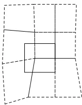
block boundary grids, which are defined on the boundaries of their parent blocks. If the grid blocks are continuous across the interface, then the block boundary grids are identical. If the grid blocks are not continuous across the interface, then a four-sided cell face belonging to the boundary grid on one side of the interface is divided intoN polygons by the boundary grid on the other side of the interface. Figure 1 shows an example of a cell being cut into 4 polygons. In the general case, a ghost cell would
Figure 1: Boundary Cell Face Being Cut by Opposing Boundary Grid
+ + +
Figure 2: Process of ”Tiling” to Form Ghost Nodes
4.2
Ghost Cell Dependent Variable Value Determination
cell with its proper value of the dependent variable u is given in Equations 35-40:
Ui1,j1,k,1 = 1
Vi1,j1,k,1
X
i2,j2
Ui2,j2,k,2¯hi1,j1,i2,j2,kAi1,j1,i2,j2 (35)
¯
hi1,j1,i2,j2,k = β1
Vi1,j1,k,1
Ai1,j1,1
+β2Vi2,j2,k,2
Ai2,j2,2
(36)
β1 = α1
α1+α2 (37)
β2 = α2
α1+α2
(38)
α1 = µ
Ai1,j1,i2,j2
Ai1,j1,1
+² ¶ µ
1− Ai1,j1,i2,j2
Ai2,j2,2
+² 
(39)
α2 = µ
Ai1,j1,i2,j2
Ai2,j2,2
+² ¶ µ
1− Ai1,j1,i2,j2
Ai1,j1,1
+² 
(40) where:
U = dependent variable vector of cell
A = area of the cell face lying on the block boundary
A = overlap area of two cell face areas
V = volume of cell
² = some small positive number.
4.3
Cell Face Intersection Area Calculation using the
Ramshaw Algorithm
The cell face intersection areas are calculated using a Ramshaw algorithm.[11] The Ramshaw algorithm stems from the general equation for the area of a polygon P:
AP = 12 Ns
X
s=1
²Ps(xs1y2s−xs2y1s) (41)
where
Ns = the number of sides
xs1, y1s = the x,y coordinates of vertex 1 of side s
xs2, y2s = the x,y coordinates of vertex 2 of side s
²Ps =
½
1 if polygon P lies to the left of side s
−1 if polygon P lies to the right of side s.
This formula allows the area of any polygon to be calculated given the locations of its vertices. Thus, if it was easy to determine all of the polygons created like the one in Figure 1, all of the overlap areas could be easily calculated. Unfortunately, the identification of these polygons is a daunting task, so an alternative method is needed.
boundary grid will have two adjacent cell faces (one on its left and one on its right) belonging to its own block boundary grid and one cell enclosing it belonging to the opposing block boundary grid. In this case, the line segment would contribute to the area defined by the overlap of two cells in its own block boundary grid with one cell of the opposing block boundary grid. Any line segment which is coincident with a line segment of the opposing block boundary grid will have two adjacent cell faces belonging to its own block boundary grid and two adjacent cell faces belonging to the opposing block boundary grid. In this case, the line segment would contribute to the area defined by the overlap of two cells in its own block boundary grid with two cells of the opposing block boundary grid. The coincidence case must be detected because it results in area contributions being counted twice, since coincident line segments ex-ist in both block boundary grids. This problem is handled by only taking one half of the contribution when a coincident line segment is detected. When the contribution of its corresponding line segment in the other block boundary grid is calculated, the other half of the contribution is recovered.
line to be divided into line segments defined by a set of nodes which are intersections of the grid line with other grid lines.
Once a line segment is defined, it is necessary to determine which cell faces are either adjacent to or enclosing it. This requires that any node defined by physical coordinates (x, y) be located in the (ξ, η) space of both of the block boundary grids. This location is performed by inverse linear transfinite interpolation using Newton’s method with line search.[12] The algorithm is given as follows:
Let~x = (x, y) and ~ξ= (ξ, η). Let~xp be the point of interest.
Define F~(~ξ) =~xA+ (~xB−~xA)(ξ− bξc) + (~xC−~xA)(η− bηc) +(~xD+~xA−~xB−~xC)(ξ− bξc)(η− bηc)−~xp. Where vertices A, B, C, D are defined as follows:
~xA←(xbξc,bηc, ybξc,bηc)
~xB ←(xbξc+1,bηc, ybξc+1,bηc)
~xC ←(xbξc,bη+1c, ybξc,bηc+1)
~xD ←(xbξc+1,bηc+1, ybξc+1,bηc+1) Start checking at location ~ξ=~ξ0. Do until ² is less than some tolerance.
∆~ξ← −(F0(~ξ))−1F~(~ξ)
λ←1
Do while kF~(~ξ+λ∆~ξ)k2 >(1−1×10⁻⁴λ)².
λ ← λ2
∆~ξ←λ∆~ξ
ξ←ξ+ max(min(∆ξ,1),0)
η←η+ max(min(∆η,1),0)
²← kF~(~ξ)k2
coincidence is severe. If a line segment belonging to one block boundary grid is labeled as being coincident with a line segment of the opposing block boundary grid, the same coincidence must be detected during the sweep through the opposing boundary grid. If this does not happen, the communication operatorsI2→1 and I1→2 will not only be wrong, but they could possibly even contain negative overlap areas.
The test for coincidence consists of calculating the perpendicular distance be-tween the end points of one line segment with the other line segment. If this distance is less than some specified tolerance ²coinc, then the line segments are deemed to be coincident. However, when the distance is very close to the tolerance, the possibility arises that this criterion could pass when sweeping through one of the block boundary grids and fail when sweeping through the other block boundary grid. Thus, a line segment AB belonging to side one of the interface could be determined to be coinci-dent with line segment CD belonging to side two of the interface during the sweep through the ξ-constant and η-constant lines of side one, whereas line segment CD would not be determined to be coincident with line segment AB during the sweep through the ξ-constant and η-constant lines of side two.
have already been projected. The algorithm is given as follows. Do until no more nodes need to be projected.
Do for both block boundary grids. Do for all nodes (x, y)i,j.
If the distance between (x, y)i,j and the closest ξ and η lines in the opposing block boundary grid is less than 2²coinc,
Project the node onto the line(s).
The closest lines mentioned in the algorithm are determined using the inverse TFI algorithm. Grid snapping does move the nodes of the meshes slightly, but as long as
²coinc is small, the movement of the nodes will not introduce significant error into the grid or solution.
4.4
Determination of
²
coincOne common problem in r-refinement algorithms is that they contain many parame-ters which are determined by the user, rather than the programmer. In the current implementation of SIERRA, there are multiple user-determined constants for each of the three stages of the algorithm (weight function calculation, node movement, and solution redistribution). This moves the burden of tuning SIERRA to the user, requiring a significant amount of trial and error. To introduce a new user-determined parameter in the communication algorithm would complicate this process further, and might even serve to make r-refinement more difficult to implement for a real problem, rather than easier. As a result of this, it is desirable for the computer to calculate ²coinc, making its effect on the algorithm transparent to the user. This is accomplished by determining²machine, and then drawing conclusions about its affect on the inverse TFI algorithm.
than this, so ²coinc is set to √3²
machine. Since the algorithm was implemented in
FORTRAN 95, the following line of code was used to calculate ²coinc:
epsilon_coinc = (nearest(1.,1.)-1.)**(1./3.).
5
Tests of the Algorithm
5.1
Static Grid Test Using the Diffusion Equation
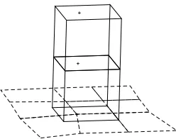
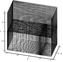
Testing of the communication algorithm on a static two-block grid with a high degree of interface discontinuity gave promising results. Figure 3 shows a 3-D plot of the grids; while Figure 4 shows a 2-D plot of the interface.
-1 -0.5 0 0.5 1
z
0
0.5
1
1.5
2
x
0 0.5
1
y
Y
X Z
Figure 3: Multiblock Grid Used in Preliminary Testing
0 0.2 0.4 0.6 0.8 1
y
0 0.5 1 1.5 2
x
Figure 4: Overlay of Surface Grids Defining the Multiblock Interface (z = 0)
-1 -0.5 0 0.5 1
z
0 0.5 1 1.5 2
x
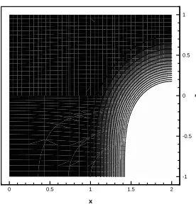
After 10000 iterations, the total mass in the system was 14.5712282575963, indicating conservation accuracy to 8 decimal places. Figure 5 shows a contour plot on a cut plane at y = 12. The plot shows that the interblock boundary (the z = 0 plane) is invisible in the solution.
5.2
Dynamic Grid Test Using the Linear Wave Equation
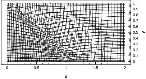
Tests of the algorithm on adaptive grids were performed to demonstrate that the algorithm is robust enough to handle dynamic discontinuities. The communication algorithm was implemented in a linear wave equation code using SIERRA to adapt the grids.[10] The block topology was the same as that of the static grid tests as shown in Figure 3. The test problem was the movement of a planar wave in the (1,1,1) direction. Figure 6 shows the two block boundary grids defining the block interface. The plot shows how the grid blocks adapt to the wave front as it passes through the interface.
0 0.1 0.2 0.3 0.4 0.5 0.6 0.7 0.8 0.9 1
y
0 0.5 1 1.5 2
x
Figure 6: Overlay of Surface Grids Defining the Multiblock Interface (z = 0)
-1 -0.5 0 0.5 1
z
0 0.5 1 1.5 2
x
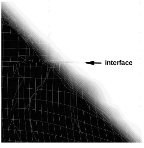
Figure 7: Contour Plot of Solution to Wave Equation at y= 12
interface
discrepancies elsewhere along the wave front due to differences in grid node density (the wave front is better resolved where the grid spacing is smaller).
5.3
Dynamic Grid Test Using the Euler Equations
Since the primary goal of developing the conservative interblock communication al-gorithm was to implement it in a CFD code, a final test of the alal-gorithm using an Euler solver coupled with SIERRA was performed. This not only demonstrated that the algorithm was stable and accurate for use in CFD applications, it also allowed the behavior of the solution to be observed.
5.3.1 Geometry for the Euler Test
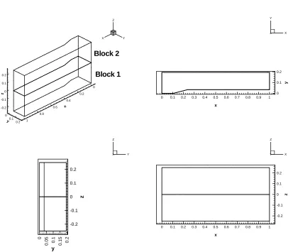
The geometry for the dynamic grid test using the Euler equations was a two block grid, each block having dimensions 161×41×5. The grids represented a 2-D channel configuration extruded in the z direction to form a 3-D channel. The inlet plane was the x = 0 plane, and this corresponded to the Imin plane in the computational space. The outlet plane was the x= 1 plane, which corresponded to the Imax plane in the computational space. The interface between the two grids was thez = 0 plane, which corresponded to theKmax plane of Zone 1 and theKmin plane of Zone 2. The
Jmin plane of both zones had a 14.5◦ wedge from (x, y) = (0.108696,0.000000) to (x, y) = (0.239130,0.033759). The Jmax plane of both zones was the y = 0.195652 plane. TheKmin plane of Zone 1 and theKmax plane of Zone 2 were thez =−0.25 and z = 0.25 planes, respectively. Figure 9 shows the geometry.
5.3.2 Initial and Boundary Conditions for the Euler Test
0 0.1 0.2
y
0 0.1 0.2 0.3 0.4 0.5 0.6 0.7 0.8 0.9 1
x X Y Z -0.2 -0.1 0 0.1 0.2 z
0 0.1 0.2 0.3 0.4 0.5 0.6 0.7 0.8 0.9 1
x Y X Z -0.2 -0.1 0 0.1 0.2 z 0 0.2 0.4 0.6 0.8 1 x 0 0.1 0.2 y X Y Z Block 2 Block 1 0 0.
05 0.1
0.
15 0.2
y -0.2 -0.1 0 0.1 0.2 z X Y Z
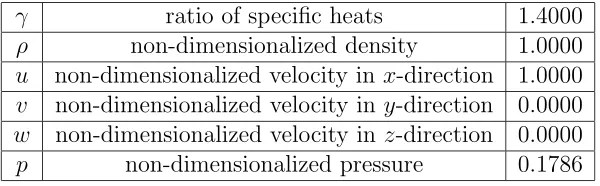
γ ratio of specific heats 1.4000
ρ non-dimensionalized density 1.0000
u non-dimensionalized velocity in x-direction 1.0000
v non-dimensionalized velocity iny-direction 0.0000
w non-dimensionalized velocity inz-direction 0.0000
p non-dimensionalized pressure 0.1786 Table 1: Inlet Conditions
outlet conditions were set using first-order extrapolation
U(ξ+ ∆ξ) = 2U(ξ)−U(ξ−∆ξ), (44)
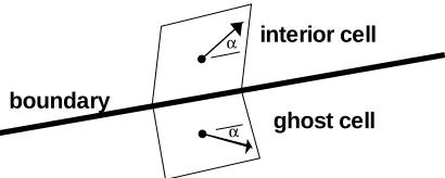
since the flow was supersonic at the exit. The boundary conditions along the inter-face between the two blocks was determined by the communication algorithm. All other block faces were given the slip boundary condition. The slip condition was implemented by using zeroth order extrapolation for ρ and p
ρ(ξ+ ∆ξ) = ρ(ξ)
p(ξ+ ∆ξ) = p(ξ), (45)
while reflecting~v across the cell face where the slip condition is being applied. Fig-ure 10 shows this reflection. The initial conditions for all interior cells were set to be the same as the inlet conditions.
5.3.3 Parameters for SIERRA
interior cell
ghost cell boundary
α
α
Figure 10: Slip Condition Being Applied to Velocity Vector
minimum allowed value ofk∇2Uk2 1×10⁻³ number of adapter iterations per flow solver step 1
subdivisions per cell in the solution
redistribution procedure 1
number of RK stages per cell subdivision 2 exponent for volume weighting (ω) 1 number of smoothing passes for weight function 8
limiter selection conservative and non-conservative variable set for non-conservative limiter conservative variables
5.3.4 Results of the Euler Test
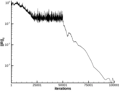
A steady-state solution for the problem was obtained. As is typically a problem with r-refinement adapters coupled with explicit solvers, the grid continued to oscillate slightly even after the shock structure was established and stationary. This caused the norm of the residual to stagnate. To prove that the residual stall was not a result of the communication algorithm, the adapter was turned off after 50000 iterations. Over the next 50000 iterations, the residual dropped to four orders of magnitude lower than the initial residual, as is shown in Figure 11. The CFL number was set
iterations
||R
||2
1 25001 50001 75001 100001
10-3
10-2
10-1
100
to 0.4, with the time step calculated as
∆t= CFL min
i,j,k
õ
|u|+a ∆x +
|v|+a ∆y +
|w|+a ∆z
¶−1!
(46)
Figure 11 is also a good demonstration for why real r-refinement applications require implicit solvers, since the increased resolution results in a very low time step for fixed CFL number.
SIERRA produced a smooth, well-adapted grid in Zone 1, which resulted in a highly mismatched interface between Zones 1 and 2. Figure 12 shows the Kmin and Kmax faces of Zones 1 and 2. Density contours on the Kmin and Kmax faces
0 0.05 0.1 0.15 0.2 y
0 0.1 0.2 0.3 0.4 0.5 0.6 0.7 0.8 0.9 1
x
X Y Z
Zone 1
KMIN(zMIN) Plane (i.e. plane farthest from the interface)
0 0.05 0.1 0.15 0.2 y
0 0.1 0.2 0.3 0.4 0.5 0.6 0.7 0.8 0.9 1
x
X Y Z
Zone 1
KMAX(zMAX) Plane (i.e. interface plane)
0 0.05 0.1 0.15 0.2 y
0 0.1 0.2 0.3 0.4 0.5 0.6 0.7 0.8 0.9 1
x
X Y Z
Zone 2
KMIN(zMIN) Plane (i.e. interface plane)
0 0.05 0.1 0.15 0.2 y
0 0.1 0.2 0.3 0.4 0.5 0.6 0.7 0.8 0.9 1
x
X Y Z
Zone 2
KMAX(zMAX) Plane (i.e. plane farthest from the interface)
Figure 12: Surface Grids on Kmin and Kmax Planes of Both Blocks
starting at the bottom of the ramp, reflecting off of the top wall in a Mach reflection, interacting with the expansion fan originating at the top of the ramp, and then going through a series of regular reflections off of the top and bottom walls before impinging on the outlet. The shock waves are very sharp on theKmin plane of Zone 1 because it is far enough away from the interface block that it is hardly affected by the unadapted block. TheKmax plane of Zone 1, however, has slightly smeared shock waves because, even though it has the ability to resolve the shocks, it is communicating with a grid that does not have the ability to resolve the shocks. The shocks are excessively smeared on theKmax plane of Zone 2 because of its lack of resolution, but theKmin plane of Zone 2 shows slightly sharper shocks because of the influence of Zone 1. Figures 14 and 15 are close-ups of the Mach reflection in Figures 12 and 13.
The influence of the communication between an adapted and unadapted block on the solution is best seen by slicing the solution in planes normal to the block interface. Figure 16 shows a composite view of density contours on sixx-constant planes. With the exception of the inlet plane (x= 0), the planes are shown individually in Figure 17. As can be seen in the figures, there are shock waves in Zone 1 which are smeared close to the interface. Likewise, there are smeared shock waves in Zone 2 which are slightly sharper close to the interface. Because of the large discrepancies in cell size across the interface near these shock waves, the contour lines are not smooth across the interface. However, the centers of the shock waves are clearly at the same place, so the discontinuous contour lines are a result of discrepancies in resolution and not a result of faulty communication between the two blocks.
5.3.5 Computational Costs in the Euler Test