Highly Efficient Computer Oriented Octree Data
Structure and Neighbors Search in 3D GIS Spatial
Noraidah Keling1, Izham Mohamad Yusoff1, Uznir Ujang2, Habibah Lateh1
1
School of Distance Education, Universiti Sains Malaysia
2
Faculty of Geoinformation & Real Estate, Universiti Teknologi Malaysia
Corresponding Author: Noraidah Keling E-mail: [email protected]
Abstract:
1 Introduction
Recent developments in the field of three-dimensional (3D) data spatial representation have led to a renewed interest in Geographic Information System (GIS). Application of 3D technologies in GIS developments is one of the issue that have special attention in this platform and has come to the limelight among various geo-related profesionals such as land practitioners and environmentalists [1][2]. Perspective in third dimension really helpful in some field likes urban planning and management [3], geological sub surface modelling [4], mining and oil exploration [5][6], hydrology [7], infrastructure modeling, geology etc [8][9]. Apart from visualization task, 3D have given new perspective in this field due to its capability of handling complex real world phenomena in more realistic manners to recognize the geographical and geological space better and master the inherent laws in earth-science and engineering application to provide facilities to analyze and thus, help decision makers explore and understand the complexities’[10]. Most of the direct and indirect approaches use GIS for effectively by incorporating GIS-functions such as a spatial database for storing, displaying, and updating the input data based on site-specific measurement and experiment to understand the role of the interaction conditioning factor [11].
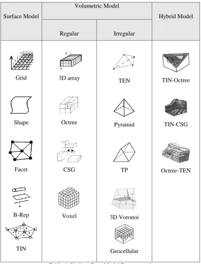
Representation of numerous real-world phenomena such as flood, geology, water pollution, air pollution in spatial data model are not same [16]. In term of geometric characteristics, existing 3D spatial representation data model in Geographical Information System (GIS) can be described by three representation which are surface, volumetric, and hybrid (mixed of both model; surface and volumetric model [4][14]. Table 1 show various data model representation [12] [17] [18][19] [20] [21] [22].
Surface Model
Volumetric Model
Hybrid Model
Regular Irregular
Grid
Shape
Facet
B-Rep
TIN
3D array
Octree
CSG
Voxel
TEN
Pyramid
TP
3D Voronoi
Geocellular
TIN-Octree
TIN-CSG
Octree-TEN
2 Methods
2.1 Related Research
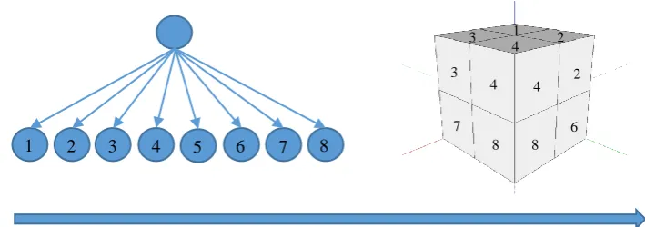
Octree is a method where 3D space had been represented in a hierarchical tree structure as visualized in Figure 1. Classical octree originate from Klinger [23] as quadtree and subsequently expanded to cover 3D space as Octree. The earlier implementation of octree use tree traversal like suggested by Samet [24], Ballard and Brown [25] and Besancon [26]. Recent research development in Octree see more effort to improve weakness of octree in finding neighbor node which is required for spatial analysis by using various address encoding scheme with specific rule like matrix [27], lookup table [28] and arithmetic [29] to eliminate the need of tree traversal.
Figure 1 : Octree Node to 3D Space Mapping
2.2 Proposed Octree Structure
In this paper, the author proposing another address encoding scheme and data structure which bases on binary ordering which efficiently preserve 3D spatial information from Octree structure and carefully designed in such way to fully take advantage of the advancement of computer CPU accelerator instruction to speed up neighbor search and eliminating the need of complex operation to derive voxel spatial information unlike suggested by Kim and Lee [29] or the matrix solution like Voros [27].
1 2 3 4 5 6 7 8
1 2 3
4 4 4
3 2
6 7
2.2.1 Binary Address Encoding
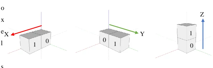
The basis of the proposed octree encoding scheme is to assign each node of Octree a unique address in binary form with 3D spatial information embedded. Octree in 3D space is binary by nature. Voxel progression along with the axis can be represent by only 1 bit as shown in Figure 2. For example, the voxel which is close to axis X, the address is set as 0 and for the voxel located further from the axis the address is set as 1. By incorporating this nature into address encoding, we can preserve all 8 v
o x e l
s
patial data information by using only 3 bits.
Figure 2 : Voxel Numbering Progression
These 3 bits can be arrange using XpYpZp standard, where P is octree level
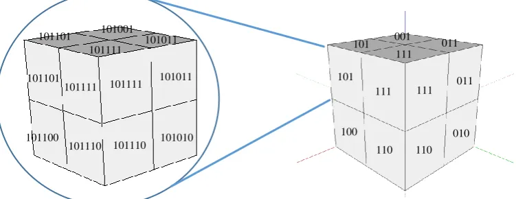
or depth. For example, for the voxel which located in coordinate x=0, y=0. z=0, the voxel address is 0b000 (0d0) and voxel located at coordinate x=1,y=0,z=1 then the voxel address will be 0b111 (0d7). The addressing for the voxel is straight forward and easy to identify voxel physical location just based on octree address. Figure 3 show the complete address for proposed octree in binary form.
Figure 3 : Proposed Octree Addressing Scheme
111 111 111
011 011 001
010 110 110 100 101
101
X
1 0 0 1
Y 1
2.2.2 Subdivision Address Encoding
Voxel Address = (XpYpZp) ᴖ (Xp+1Yp+1Zp+1) ᴖ …. ᴖ (Xp+nYp+nZp+n)
(1)
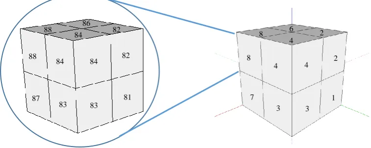
The address encoding for subdivision octree is similar with parent voxel except the parent address is directly concatenating into child voxel address as shown in (1). The main different between proposed encoding with previous methods that introduced by Voros [27], Payeur [28] and Kim & Lee [29] is this method stricly using 3 bits binary encoding per level as shown in Figure 4 and Figure 5 while others are using decimal based as shown in Figure 6 and Figure 7. Decimal representation is make sense for human readable and manual processing because parent address can be easily identified concatenated with child address, but to represent those number in decimal will require 25% more space and without any advantage for computer processing.
Figure 4 : Proposed Octree Subdivision Addressing Scheme (binary)
111 111 111
011 011 001
010 110 110 100 101
101
101111 101111 101011 101011
101101 101101
101111 101001
101110 101100
Figure 5 : Proposed Octree Subdivision Addressing Scheme (hexadecimal)
Figure 6 : Payeur and Voros Octree Subdivision Addressing Scheme
Figure 7 : Kim and Lee Octree Subdivision Addressing Scheme
7 7 7 3 3 1 2 6 6 4 5 5
2F 2F 2B
2B 2D 2D 2F 29 2E 2C 2E 2A 7 7 7 3 3 1 2 6 6 4 5 5
57 57 53
53 55 55 57 51 56 54 56 52 4 4 4 2 2 6 1 3 3 7 8 8
84 84 82
2.3 Data Structure
In order to take advantage of modern computer (explained in section 2.4), each voxel should be kept either in 32 bits or 64 bits. By using equation (2), 32 bits data structure able to hold maximum of 10 levels of octree and for 64 bits data structure will to be able to hold up to 21 levels of octree.
(2)
Using equation (3), with the assumption of minimum resolution of surface area that we want to cover is 1 m2, 32bits data structure only able to cover up to 1,048.576 km2 but 64 bits data structure able to cover up to 4,398,046,511.104km2. With the total earth surface area is estimated only around 510,072,000 km2, 64 bits data structure practically more than enough to cover whole earth thus there is no need more than 64 bits data structure.
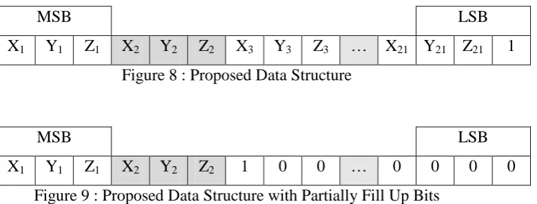
(3) For this paper, we focus on 64 bits data structure but the same method also can be applied for 32 bits data structure. The octree node address XpYpZp for
each level should be start concatenated from MSB to LSB with 0b1 appended after last 3 bits address as terminator as shown in Figure 8 and Figure 9.
MSB LSB
X1 Y1 Z1 X2 Y2 Z2 X3 Y3 Z3 … X21 Y21 Z21 1
Figure 8 : Proposed Data Structure
MSB LSB
X1 Y1 Z1 X2 Y2 Z2 1 0 0 … 0 0 0 0
Numbers of octree level can be determine by (4) and since each level require 3 bits of information embedded into the data structure, the total of bits need to be used is calculated according to (5).
(( ))
(4)
+ 1
(5)
2.4 CPU Accelerated Instruction
Bit Manipulation Instruction 2 (BMI2) is series of new instructions introduced by Intel as part of Advance Vector Extensions 2 (AVX 2) in 2013 [30]. The same instruction and also supported by AMD in Excavator 2015. Intel and AMD is market leader in computing with 80% of the total computer sold is based on Intel or AMD CPU. There are 3 instructions from BMI2 that can be used to accelerate octree address generation and manipulation; TZCNT, PDEP and PEXT.
2.4.1 Count the Number of Trailing Zero Bits (TZCNT)
TZCNT is a single instruction to count trailing 0 in the registers. This instruction eliminating the need of bit extraction-compare loops as shown in Figure 10. TZCNT can be used to identify octree level from voxel address as demonstrate in section 2.5.1
temp ← 0
DEST ← 0
DO WHILE ( (temp < OperandSize) and (SRC[ temp] = 0) )
temp ← temp +1
DEST ← DEST+ 1
OD
CF ← 1
ELSE
CF ← 0
FI
IF DEST = 0
ZF ← 1
ELSE
ZF ← 0
FI
Figure 10 : TZCNT Pseudo Code
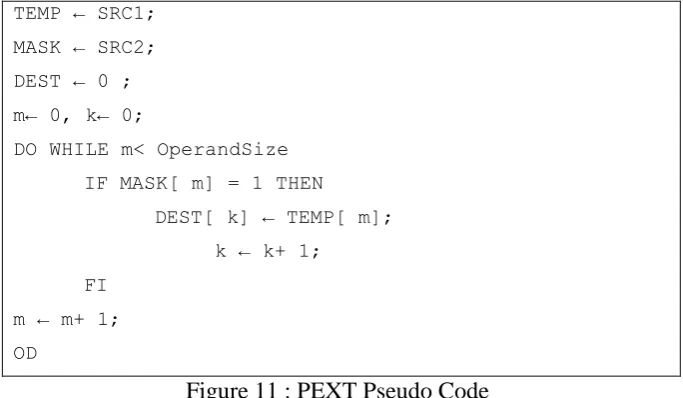
2.4.2 Parallel bits Extract (PEXT)
PEXT is a single instruction to insert bits into different position from a sequences as shown in Figure 11. PEXT use in proposed method to reconstruct voxel address as demonstrate in section 2.5.2 and 2.5.4.
TEMP ← SRC1;
MASK ← SRC2;
DEST ← 0 ;
m← 0, k← 0;
DO WHILE m< OperandSize
IF MASK[ m] = 1 THEN
DEST[ k] ← TEMP[ m];
k ← k+ 1;
FI
m ← m+ 1;
OD
Figure 11 : PEXT Pseudo Code
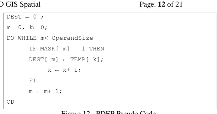
2.4.3 Instructions, Parallel Bits Deposit (PDEP)
PDEP is a single instruction to gather bits from different position into a sequences as shown in Figure 12. PDEP use in proposed method to extract X Y and Z 3D spatial coordinate from voxel address as demonstrate in section 0 and 2.5.4
TEMP ← SRC1;
DEST ← 0 ;
m← 0, k← 0;
DO WHILE m< OperandSize
IF MASK[ m] = 1 THEN
DEST[ m] ← TEMP[ k];
k ← k+ 1;
FI
m ← m+ 1;
OD
Figure 12 : PDEP Pseudo Code 2.5 Manipulation
2.5.1 Determine Octree Level from Voxel Address
Using proposed voxel address encoding and data structures, we can easily determine octree level from voxel address alone without requiring whole octree traversal. Here TZCNT can help to determine location of termination bit as shown in Figure 13.
MSB LSB
X1 Y1 Z1 … X19 Y19 Z19 X20 Y20 Z20 1 0 0 0
0 0 0 … 0 0 0 0 0 0 0 0 1 1
MSB LSB
Figure 13 : Counting Trailing Zeros
After getting termination bit location, octree level can be determine by using (6)
(6)
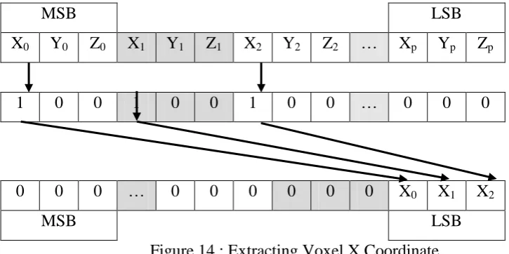
2.5.2 Voxel Address to 3D Spatial Coordinate
(7) Figure 14 visualize how X axis coordinate can be extracted from voxel address. The same process also true for Y and Z axis as shown in Figure 15 and Figure 16.
MSB LSB
X0 Y0 Z0 X1 Y1 Z1 X2 Y2 Z2 … Xp Yp Zp
1 0 0 1 0 0 1 0 0 … 0 0 0
0 0 0 … 0 0 0 0 0 0 X0 X1 X2
MSB LSB
Figure 14 : Extracting Voxel X Coordinate
MSB LSB
X0 Y0 Z0 X1 Y1 Z1 X2 Y2 Z2 … Xp Yp Zp
0 1 0 0 1 0 0 1 0 … 0 0 0
0 0 0 … 0 0 0 0 0 0 Y0 Y1 Y2
MSB LSB
MSB LSB X0 Y0 Z0 X1 Y1 Z1 X2 Y2 Z2 … Xp Yp Zp
0 0 1 0 0 1 0 0 1 … 0 0 0
0 0 0 … 0 0 0 0 0 0 Z0 Z1 Z2
MSB LSB
Figure 16 : Extracting Voxel Z Coordinate
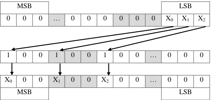
2.5.3 3D Spatial Coordinate to Voxel Address
For application that need voxel address generation for certain voxel coordinate like voxel neighbor discovery, PDEP can be used efficiently to reconstruct voxel address as shown in (8).
(8)
Figure 17 visualize how X axis coordinate can be converted into voxel address. The same process also true for Y and Z axis as shown in Figure 18 and Figure 19.
MSB LSB
0 0 0 … 0 0 0 0 0 0 X0 X1 X2
1 0 0 1 0 0 1 0 0 … 0 0 0
X0 0 0 X1 0 0 X2 0 0 … 0 0 0
MSB LSB
MSB LSB
0 0 0 … 0 0 0 0 0 0 Y0 Y1 Y2
0 1 0 0 1 0 0 1 0 … 0 0 0
X0 Y0 0 X1 Y1 0 X2 Y2 0 … 0 0 0
MSB LSB
Figure 18 : Voxel Address Generation for Y Axis
MSB LSB
0 0 0 … 0 0 0 0 0 0 Z0 Z1 Z2
0 0 1 0 0 1 0 0 1 … 0 0 0
X0 Y0 Z0 X1 Y1 Z1 X2 Y2 Z2 … 0 0 0
MSB LSB
Figure 19 : Voxel Address Generation for Z Axis
2.5.4 Finding Neighbor Voxel
Figure 20 : 26 Neighbors Voxels
use octree in those situation, address encoding like by proposed Voros [27], Payeur [28] and Kim & Lee [29] is favored.
There are total of 26 neighbor voxels in an Octree and the offset of XYZ coordinate is shown in Figure 20. Our proposed method able to find each of them with 3 simple generic step without complicated math or lookup table. For example, to get neighbor address at offset +X+Y+Z:
1) Extract voxel reference coordinate Xref= PEXT (X mask, Voxelref)
Yref= PEXT (Y mask, Voxelref)
Zref= PEXT (Z mask, Voxelref)
2) Add neighbor offset X+X+Y+Z = Xref + 1
Y+X+Y+Z = Yref + 1
Z+X+Y+Z = Zref + 1
3) Reconstruct Voxel+X+Y+Z address
Voxel+X+Y+Z = PDEP(X Mask, X+X+Y+Z) PDEP(X Mask, Y+X+Y+Z)
PDEP(X Mask, Z+X+Y+Z)
Our proposed method also having fixed complexity regardless octree level so it suit for simple and huge octree structure.
3 Results
neighbor search for those alternative implementation and our proposed
method.
Figure 21: Worst Case Complexity of Neighbor Search
Another advantage to for having data structure and encoding that computer friendly is the ability to speedup address encoding, extraction and neighbor search with BMI2 instruction which is very fast and simpler to implement compared with generic implementation. Figure 22 show comparison of performance between generic implementation and BMI2 accelerated instruction. By average, BMI2 implementation 700% faster than generic implementation.
1 10 100 1000 10000 100000
1 2 3 4 5 6
WORST CASE COMPLEXITY VS OCTREE
LEVEL
Figure 22 : Octree Neighbor Finding Performance Improvement with BMI2 4 Discussion
The key for faster and simple octree address encoding scheme is to use binary form. Octree in 3D space is binary compatible and by using clever rule, 3D spatial information easily embed inside the address itself and can be
constructed, extracted and manipulated without using complex post
processing. We also proposing new 64 bits data structure which is designed with BMI2 compatible in mind and proposing simple and fast method for neighbor search which is having constant complexity regardless octree level. This method can be expanded in the future to cover the neighbor search for intra octree level.
0 10 20 30 40 50
1 0 0 0 2 0 0 0 4 0 0 0 8 0 0 0 1 0 0 0 0 2 0 0 0 0 4 0 0 0 0
IMPLEMENTATION PERFORMANCE
(TIME TO COMPLETE (MS))
References
[1] M. F. Goodchild, ―Geographic information systems and science: today and tomorrow,‖ Annals of GIS, vol. 15. pp. 3–9, 2009.
[2] B. J. L. Berry, D. A. Griffith, and M. R. Tiefelsdorf, ―From Spatial Analysis to Geospatial Science,‖ vol. 40, pp. 229–238, 2008.
[3] U. Ujang, A. A. Rahman, and F. Anton, ―An Approach of Instigating 3D City Model s i n Urban Air Pollution Modeling for Sustainable Urban Development in Malaysia An Approach of Instigating 3D City Model s i n Urban Air Pollution Modeling f or Sustainability Urban Development in Malaysia,‖ no. June 2014, pp. 1–22.
[4] L. Q. R. Li, Y. Chen, F. Dong, ―3D Data Structures and Applications in Geolofical Subsurface Modeling,‖ in International Archives of
Photogrammetrry and Remote Sensing. Vol. XXXI, Part B4. Vienna, 1996, pp. 508–513.
[5] J. Pouliot, K. Bédard, D. Kirkwood, and B. Lachance, ―Reasoning about geological space: Coupling 3D GeoModels and topological queries as an aid to spatial data selection,‖ Comput. Geosci., vol. 34, pp. 529–541, 2008. [6] B. Jin, Y. Fang, and W. Song, ―3D visualization model and key techniques
for digital mine,‖ Trans. Nonferrous Met. Soc. China, vol. 21, pp. s748– s752, 2011.
[7] M. Y. Izham, U. Muhamad Uznir, A. R. Alias, K. Ayob, and I. Wan Ruslan, ―Influence of georeference for saturated excess overland flow modelling using 3D volumetric soft geo-objects,‖ Comput. Geosci., vol. 37, no. 4, pp. 598–609, Apr. 2011.
[8] L. F. Zhu, M. J. Li, C. L. Li, J. G. Shang, G. L. Chen, B. Zhang, and X. F. Wang, ―Coupled modeling between geological structure fields and property parameter fields in 3D engineering geological space,‖ Eng. Geol., vol. 167, pp. 105–116, 2013.
[9] L. Zhu, C. Zhang, M. Li, X. Pan, and J. Sun, ―Building 3D solid models of sedimentary stratigraphic systems from borehole data: An automatic method and case studies,‖ Eng. Geol., vol. 127, pp. 1–13, 2012.
[10] H. Tianding, ―3D GIS interactive editing method: Research and application in glaciology,‖ … Sci. Eng. (ICISE), 2010 2nd …, pp. 1–4, 2010.
[11] R. a de By, ―Principles of Geographic Information Systems---An introductory textbook,‖ vol. 1, 100AD.
[13] J. D. Rogers and R. Luna, ―IMPACT OF GEOGRAPHICAL
INFORMATION SYSTEMS ON GEOTECHNICAL ENGINEERING,‖ pp. 1–23, 2004.
[14] W. Lixin, ―Topological relations embodied in a generalized tri-prism (GTP) model for a 3D geoscience modeling system,‖ Comput. Geosci., vol. 30, pp. 405–418, 2004.
[15] S. H. I. Wenzhong, ―DEVELOPMENT OF A HY BRID MODEL FOR THREE-DIMENSIONAL GIS,‖ Geo-Spatial Inf. Sci., vol. 3, pp. 6–12, 2000.
[16] M. Breunig and S. Zlatanova, ―3D geo-database research: Retrospective and future directions,‖ Comput. Geosci., vol. 37, no. 7, pp. 791–803, Jul. 2011.
[17] D. Y. Shen, A. N. Ma, H. Lin, X. H. Nie, S. J. Mao, B. Zhang, and J. J. Shi, ―A new approach for simulating water erosion on hillslopes,‖ International Journal of Remote Sensing, vol. 24. pp. 2819–2835, 2003.
[18] D. Y. Shen, K. Takara, Y. Tachikawa, and Y. L. Liu, ―3D simulation of soft geo‐objects,‖ Int. J. Geogr. Inf. Sci., vol. 20, no. 3, pp. 261–271, Mar. 2006.
[19] D. Shen and K. Takara, ―A modelling and 3-D simulation system for water erosion on hillslopes—M3DSSWEH,‖ J. Hydraul. Res., vol. 44, no. 5, pp. 674–681, Sep. 2006.
[20] W. U. Huixin and X. U. E. Huifeng, ―A New Hybrid Data Structure for 3D GIS,‖ First Int. Conf. Innov. Comput. Inf. Control - Vol. I, vol. 1, pp. 162– 166, 2006.
[21] S. Wenzhong, ―Development of a hybrid model for three-dimensional GIS,‖ Geo-Spatial Inf. Sci., vol. 3, pp. 6–12, 2000.
[22] D. Shen, D. W. Wong, F. Camelli, and Y. Liu, ―An ArcScene plug-in for volumetric data conversion, modeling and spatial analysis,‖ Comput. Geosci., vol. 61, pp. 104–115, 2013.
[23] A. Klinger, ―Patterns and search statistics,‖ Optim. methods Stat., 1971. [24] H. Samet, ―Neighbor finding in images represented by octrees,‖ Comput.
Vision, Graph. Image Process., vol. 45, p. 400, 1989.
[25] D. Ballard and C. Brown, ―Computer vision, 1982,‖ Prenice-Hall, Englewood Cliffs, NJ.
[27] J. Vörös, ―Strategy for repetitive neighbor finding in octree
representations,‖ Image Vis. Comput., vol. 18, pp. 1085–1091, 2000. [28] P. Payeur, ―A computational technique for free space localization in 3-D
multiresolution probabilistic environment models,‖ IEEE Trans. Instrum. Meas., vol. 55, no. 5, pp. 1734–1746, 2006.
[29] J. Kim and S. Lee, ―Fast neighbor cells finding method for multiple octree representation,‖ 2009 IEEE Int. Symp. Comput. Intell. Robot. Autom. -, pp. 540–545, Dec. 2009.
[30] I. Intel, ―Advanced vector extensions programming reference,‖ Intel Corp., 2011.
[31] P. Payeur, ―An optimized computational technique for free space
localization in 3-D virtual representations of complex environments,‖ 2004 IEEE Symp. Virtual Environ. Human-Computer Interfaces Meas. Syst. 2004. (VCIMS)., no. AUGUST 2004, pp. 1–7, 2004.
[32] I. Gargantini, ―Linear octtrees for fast processing of three-dimensional objects,‖ Comput. Graph. Image Process., 1982.