Addressing Computational Complexity of Electromagnetic Systems Using Parameterized Model Order Reduction

Western University Western University

Scholarship@Western

Scholarship@Western

Electronic Thesis and Dissertation Repository

August 2010

Addressing Computational Complexity of Electromagnetic

Addressing Computational Complexity of Electromagnetic

Systems Using Parameterized Model Order Reduction

Systems Using Parameterized Model Order Reduction

Majid Ahmadloo

University of Western Ontario

Supervisor

Dr. Anestis Dounavis

The University of Western Ontario

Graduate Program in Electrical and Computer Engineering

A thesis submitted in partial fulfillment of the requirements for the degree in Doctor of Philosophy

© Majid Ahmadloo 2010

Follow this and additional works at: https://ir.lib.uwo.ca/etd

Part of the Electromagnetics and Photonics Commons, and the VLSI and Circuits, Embedded and Hardware Systems Commons

Recommended Citation Recommended Citation

Ahmadloo, Majid, "Addressing Computational Complexity of Electromagnetic Systems Using Parameterized Model Order Reduction" (2010). Electronic Thesis and Dissertation Repository. 12.

https://ir.lib.uwo.ca/etd/12

This Dissertation/Thesis is brought to you for free and open access by Scholarship@Western. It has been accepted for inclusion in Electronic Thesis and Dissertation Repository by an authorized administrator of

Addressing Computational Complexity of

Electromagnetic Systems Using Parameterized Model Order

Reduction

(Spine Title: Numerical Reduction Techniques for

Electromagnetic Systems)

(Thesis format: Monograph)

by

Majid Ahmadloo

Graduate Program in Engineering Science

Department of Electrical and Computer Engineering

A THESIS SUBMITTED TO THE FACULTY OF GRADUATE STUDIES AND RESEARCH IN PARTIAL FULLFILMENT OF THE REQUIREMENTS FOR THE

DEGREE OF DOCTOR OF PHILOSOPHY

THE SCHOOL OF GRDAUATE AND POSTDOCTORAL STUDIES THE UNIVERSITY OF WESTERN ONTARIO, LONDON, ONTARIO, CANADA

THE UNIVERSITY OF WESTERN ONTARIO

SCHOOL OF GRADUATE AND POSTDOCTORAL STUDIES

CERTIFICATE OF EXAMINATION

Supervisor

______________________________ Dr. Anestis Dounavis

Supervisory Committee

______________________________

Examiners

______________________________ Dr. Kazimierz Adamiak

______________________________ Dr. Jayshri Sabarinathan

______________________________ Dr. Anand V. Singh

______________________________ Dr. Mustapha C. E. Yagoub

The thesis by

Majid Ahmadloo

entitled:

Addressing Computational Complexity of Electromagnetic Systems

Using Parameterized Model Order Reduction

is accepted in partial fulfilment of the requirements for the degree of

Doctor of Philosophy

Abstract

As operating frequencies increase, full wave numerical techniques such as the finite

element method (FEM) become necessary for the analysis of high-frequency and

microwave circuit structures. However, the FEM formulation of microwave circuits often

results in very large systems of equations which are computationally expensive to solve.

The objective of this thesis is to develop new parameterized model order reduction

(MOR) techniques to minimize the computational complexity of microwave circuits.

MOR techniques provide a mechanism to generate reduced order models from the

detailed description of the original FEM formulation.

The following contributions are made in this thesis:

1. The first project deals with developing a parameterized model order reduction to

solve eigenvalue equations of electromagnetic structures that are discretized by using

FEM. The proposed algorithm uses a multidimensional subspace method based on

modified perturbation theory and singular-value decomposition to perform reduction

directly on the finite element eigenvalue equations. This procedure generates

parametric reduced order models that are valid over the desired parameter range

without the need to redo the reduction when design parameters are changed. This

provides significant computational savings when compared to previous eigenvalue

MOR techniques, since a new reduced order model is not required each time a design

parameter is changed.

2. Implicit moment match techniques such as the Arnoldi algorithm are often used to

improve the accuracy of the reduced order model. However, the traditional Arnoldi

arbitrary functions of frequency due to material and boundary conditions. In this

work, an efficient algorithm to create parametric reduced order models of distributed

electromagnetic systems that have arbitrary functions of frequency (due to material

properties, boundary conditions, and delay elements) and design parameters. The

proposed method is based on a multi-order Arnoldi algorithm used to implicitly

calculate the moments with respect to frequency and design parameters, as well as the

cross-moments. This procedure generates parametric reduced order models that are

valid over the desired parameter range without the need to redo the reduction when

design parameters are changed and provides more accurate reduced order systems

when compared with traditional approaches such as Modified Gram Schmidt.

3. This project develops an efficient technique to calculate sensitivities of microwave

structures with respect to network design parameters. The proposed algorithm uses a

parametric reduced order model to solve the original network and an adjoint variable

method to calculate sensitivities. Important features of the proposed method are 1)

that the solution of the original network as well as sensitivities with respect to any

parameter is obtained from the solution of the reduced order model, and 2) a new

Acknowledgement

This thesis could not be successful without the invaluable support of my supervisor

Dr. Anestis Dounavis of the Department of Electrical and Computer Engineering,

University of Western Ontario. I would like to express my gratitude towards him for

introducing me to the area of model order reduction and imbibing in me the enthusiasm

for research. His motivation, keen acumen in this field of research and friendly

disposition has always had a positive effect on my work.

I would also like to extend my thanks towards every faculty member, staff member

and friend of the Department of Electrical and Computer Engineering, University of

Western Ontario for their support and help at various stages of my thesis work. I would

like to specially mention my colleagues Amir Beygi and Ehsan Rasekh and Sourajeet

Roy for their invaluable advice.

My final thoughts are with my parents, Abolghasem and Fatemeh. Without their

encouragement and endless support, I would not have had the opportunity to complete

Contents

Certificate of Examination………...……... ii

Abstract………...…..…………. iii

Acknowledgements………...……….. v

Contents………. vi

List of Tables………...… viii

List of Figures ………...……..…….. ix

Abbreviations………...……….. xi

1. Introduction………..………. 1

1.1. Background and Motivation………….………1

1.2. Objectives………..……….. 4

1.3. Contributions……….……….………. 6

1.4. Organization of Thesis……….……… 7

2. Background and Literature Review……….... 9

2.1. Introduction………..……… 9

2.2. Simulation of Microwave Systems……….………..……. 10

2.2.1. FEM formulation of Microwave Systems………..………. 11

2.3. Simulation Techniques based on MOR……….……… 15

2.3.1. SVD Based MOR on Eigenproblems………….……….………... 16

2.3.2. Moment Matching Based MOR………..… 18

2.3.3. Sensitivity Analysis Using MOR Techniques………..….. 24

3. Parameterized Model Order Reduction on Eigenvalue Equations……… 27

3.1. Introduction………..…….. 27

3.2. Formulation of microwave system………..……... 27

3.3. Parameterized Reduced Order Model………..…….. 28

3.3.1. Parametric System Formulation………..…… 28

3.3.2. Computation of Parameterized Reduced Order Model………..……….29

3.3.3. Selecting the Order of the Reduced Order Model………..……… 34

3.4. Numerical Examples………..… 35

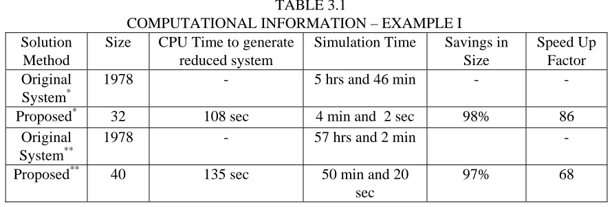
3.4.1. Example I: Partially-Filled Rectangular Waveguide………..……… 35

3.4.2. Example II: Microstrip Line………..…………. 40

4. Parameterized Model Order Reduction of Electromagnetic Systems using Multi-Order Arnoldi……….. 45

4.1. Introduction………..…….. 45

4.2. Parameterized Multi-Order Arnoldi for Systems with Arbitrary Functions…..…… 46

4.2.1. Computation of Reduced Order Model………..…. 46

4.2.2. Selecting the Order of the Reduced Order Model………..… 54

4.3. Problem Formulation and Numerical Examples………..…..55

4.3.1. Example I: RLC Network with Delay Elements………... 55

5. Sensitivity Analysis of Microwave Circuits using Parameterized Model Order

Reduction Techniques……… 66

5.1. Introduction………..……...66

5.2. Formulation of Microwave System………... 67

5.2.1. Adjoint Variable Method using MOR……… 67

5.2.2. Sensitivity Analysis of S-Parameters……….. 69

5.3. Numerical Example………..………. 71

6. Conclusion and Future Research……….. 85

6.1. Conclusion………..……... 85

6.2. Suggestions for Future Research………..……. 86

References……… 87

List of Tables

TABLE 3.1. ………..… 38

TABLE 3.2. ………..……… 44

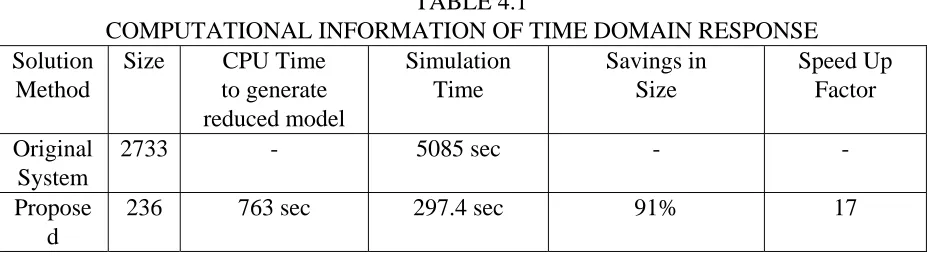
TABLE 4.1. ……….……. 60

TABLE 4.2. ………..……… 65

List of Figures

Fig.2.1. Block Arnoldi Algorithm for expansion about a complex frequency point

0 s

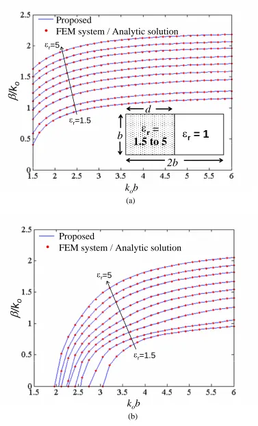
s= ………. 22 Fig. 3.1. Dielectric-loaded rectangular waveguide and the dispersion curves of the lowest four modes as εr ranges from 1.5 to 5 (a) mode 1 and physical geometry of waveguide (b)

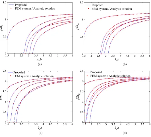
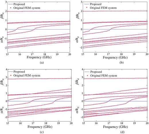
mode 4………... 34 Fig.3.2. Dispersion curves of the lowest five modes at the four extreme corners of parameter ranges for εr and d (a) At εr =1.5 and d=b (b) At εr =1.5 and d=1.3b (c) At εr

=5 and d=b (d) At εr =5 and d=1.3b………...………... 35

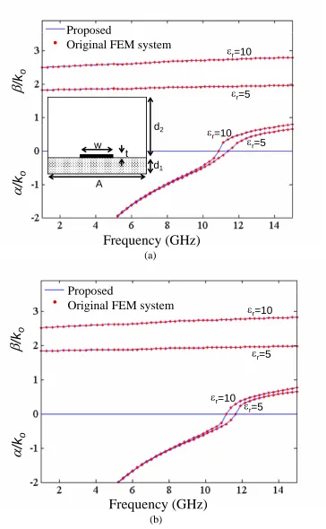
Fig. 3.3. Lossless microstrip line and the dispersion curves of the first two modes at the four extreme corners of parameter ranges for εr and w (a) At w=1.27 mm for εr =5 and εr

=10, (b) At w=1.65 mm for εr =5 and εr =10. In all cases A=12.7 mm, d1=1.27 mm,

d2=11.43 mm and t=0.127 mm………. 40

Fig. 3.4. Dispersion curves of the lowest twelve modes at the four extreme corners of parameter ranges for εr and w (a) At εr =5 and w=1.27 mm (b) At εr =5 and w=1.65 mm

(c) At εr =10 and w=1.27 mm (d) At εr =10 and w=1.65 mm………. 41

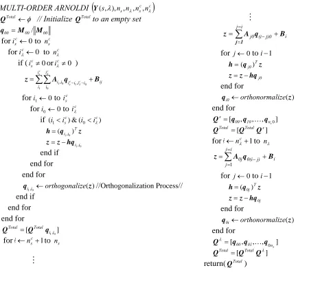
Fig. 4.1. Multi-Order Block Arnoldi Procedure including self-terms; with respect to frequency s, the design parameter λand the cross-terms………. 49 Fig.4.2. Multi-Order Block Arnoldi Procedure including self-terms; with respect to design parameters λN,K,λ0and the cross-terms……… 50

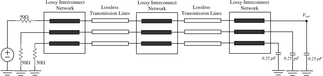
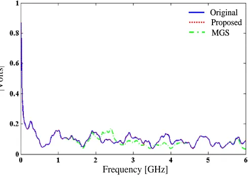
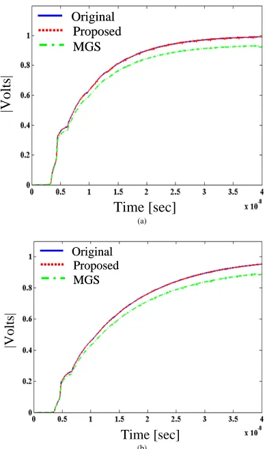
Fig. 4.3. RLC network including delay elements………. 55 Fig. 4.4. Frequency responses of the system of example 1 at the far end point at the expansion point at T = 5°C………... 56 Fig. 4.5. Time domain response of the system of example 1 at the far end point, at (a) T =

°

−40 C and (b) T = 50°C………... 57 Fig. 4.6. Geometry of the dual inductive iris filter………... 59 Fig. 4.7. The magnitude of S21 as a function of frequency at the expansion point at the

mid-range of design parametersεrandσ ……….. 60

Fig. 4.8. The magnitude of S21 as a function of frequency for different parameter values at

the corner of design parameters; (a) εr=1 and σ =3.78e7, (b)εr=5 and σ =3.78e7,

(c)εr=1 and σ =6.301e7 and (d) εr=5 and σ=6.301e7………... 61

Fig.5.1. WR90 waveguide with metallic iris at the input port. The rest of the waveguide is filled with dielectric material……… 70 Fig. 5.2a. S11 of the waveguiding structure at extreme corners of parameter ranges for εrand w (a)

r

ε =1 and w=0.00386, (b) εr=1 and w=0.00586………..………. 73

Fig. 5.2b. S₁₁ of the waveguiding structure at extreme corners of parameter ranges for εrand w

(a) εr=5 and w=0.00386 and (b) εr=5 and w=0.00586……… 74

Fig. 5.3a. ∠S11 of the waveguiding structure at extreme corners of parameter ranges for εrand w

(a) εr=1 and w=0.00386, (b) εr=1 and w=0.00586……….. 75

Fig. 5.3b. ∠S₁₁ of the waveguiding structure at extreme corners of parameter ranges for εrand w

Fig. 5.4a. Sensitivities of S₁₁ of the waveguiding structure with respect to εrat (a) εr=3,

w=0.00386, (b) εr=3, w=0.00586………. 77

Fig. 5.4b. Sensitivities of ∠S11of the waveguiding structure with respect to εrat (a) εr=3,

w=0.00386, (b) εr=3, w=0.00586………. 78

Fig. 5.5a. Sensitivities of S11 of the waveguiding structure with respect to w at (a) εr=1,

w=0.00486, (b) εr=5, w=0.00486………. 79

Fig. 5.5b. Sensitivities of ∠S₁₁of the waveguiding structure with respect to w at (a) εr=1,

Abbreviations

AWE Asymptotic Waveform Evaluation.

CFH Complex Frequency Hopping.

EM Electromagnetic.

FEM Finite Element Method.

LU Lower-upper matrix decomposition.

MGS Modified Gram Schmidt.

MOR Model Order Reduction.

ODE Ordinary Differential Equation.

PDE Partial Differential Equation.

PEC Perfect Electric Conductor.

PMC Perfect Magnetic Conductor.

p.u.l. Per-unit-length.

RF Radio Frequency.

SVD Singular Value Decomposition.

TEM Transverse electromagnetic.

Chapter 1

1. Introduction

1.1. Background and Motivation

The rapid advances of high frequency circuit technology have significantly affected the

construction of different types of microwave, millimeter-wave, optical and VLSI devices

commonly used in mobile communications, radio links, optical communications, and

various other automotive electronics systems. Modern wireless systems involve

electrically large electromagnetic (EM) structures such as the waveguides, antennas,

microwave circuits, and optical components, which are very complex in both geometry

and material properties [1]. Also technological advances in the circuit technology have

significantly reduced the feature sizes of high-speed electronic circuits and increased the

density of chips. This leads to the need for efficient analysis and design tools for

simulating and modeling the behavior of such structures and also performing

optimization on the parameters of such devices prior to costly prototype development.

Moreover, circuit designers also demand that the simulation techniques be fast and run on

relatively small computing platforms, such as standard desktop personal computers [1].

Hence at higher frequencies, integrated and microwave circuits require fast and accurate

modeling and simulation techniques for the optimization and design space exploration

problems.

The design of electromagnetic devices such as wave-guiding structures, microstrip

Differential Equations (PDE)s such as the vector wave equation derived by Maxwell’s

equations and hence full wave techniques are required to accurately characterize these

systems [2]-[6]. Numerical methods, such as the Finite Element Method (FEM), have

become extensively popular for accurate full wave analysis of microwave waveguide

devices [2]-[6]. The key advantages of the FEM are the accuracy, versatility and its

ability to handle complex materials (including anisotropic, lossy, non-linear etc) and

complicated geometries [2]-[4]. However it relies on the discretization of three

dimensional space and thus results in very large systems of equations which are

prohibitively expensive to solve. Furthermore, these equations are solved for a wide

frequency band and at different design parameters. One way to address computational

complexity of FEM is based on Model Order Reduction (MOR) techniques [7]-[19],

[28]-[30]. MOR techniques have been developed to efficiently calculate the scattering

parameters [11]–[12], [14]-[16], [19] and to perform fast wideband eigenmode analysis

of electromagnetic devices [28]–[31]. These algorithms are able to capture the frequency

response of large linear networks with low-order rational approximations. The underlying

concept of MOR is that distributed networks usually have large number of poles,

however, only a small percentage of these poles is dominant. Dominant poles are defined

as poles that have significant influence in the behavior of the network. By capturing only

the dominant poles, the CPU expense of the simulation can be significantly reduced

without compromising accuracy.

MOR techniques provide a mechanism to generate reduced order models from the

detailed description of the original FEM network. This is achieved by using moment

original system to approximate the response with a low-order transfer function [12],

[14]-[17], [19], [21]-[30]. However, these numerical techniques all conserve the original

system moments only with respect to frequency. While this provides a significant CPU

cost advantage when performing a single frequency sweep, a new reduced order model is

required each time a parameter is varied in the structure under study. This results in a

significant overhead and reduced efficiency when performing common design steps such

as optimization and design space exploration. Parameterized model order reduction

techniques have been proposed in the circuit area to address such concerns which

produce reduced order models that are functions of frequency or time as well as other

design parameters [20]-[26]. However, parameterized MOR techniques have not been

developed to solve microwave systems described by FEM equations.

Reduced order models are accurate at the frequency point of expansion and less

accurate away from the expansion point. To increase the accuracy of the reduced order

model additional moments are required or multiple expansion points can be used [43]. An

issue in developing efficient reduced order models is that as the number of moments

increases, the moments become ill-conditioned due to the fact that the higher order

moments converge to the largest eigenvalue of the system and are almost identical or

parallel to each other [43]-[44]. This minimizes the efficiency of the reduced order

model. One approach to improve the conditioning of the moment generating process is to

use implicit moment matching techniques such as the Arnoldi process [43]-[44]. The

traditional Arnoldi algorithm is applicable to first order linear systems that have a linear

dependency with respect to frequency. However, distributed microwave systems are

frequency due to material properties and boundary conditions. As a result, traditional

Arnoldi algorithms are not directly applicable in calculating the moments of the reduced

order system for microwave systems that exhibit arbitrary functions of frequency due to

high frequency phenomena such as skin effect.

MOR techniques have also been applied to perform sensitivity analysis of distributed

interconnects and microwave systems [80], [89]-[90]. However, these MOR-sensitivity

algorithms capture only the frequency moments of the original system. As a result, a new

reduced order model is required each time a design parameter is modified, which can

significantly increases the overhead of the optimization process.

The next sections describe the objectives and contributions of this thesis.

1.2. Objectives

The objective of this thesis is to develop efficient modeling techniques for the EM

structures and high frequency microwave circuit simulation. The proposed methodology

uses parameterized MOR techniques to reduce the computational complexity of

microwave systems described by the FEM formulation.

The FEM model used for microwave systems is obtained from the vector wave

equation for the electric field derived from Maxwell’s equation [27]. FEM discretization

of the vector wave equation results in a very large system of equations that are inherently

time consuming to solve. MOR techniques have been proposed in literature to

significantly reduce the CPU time required to simulate these large scale FEM problems

[11]–[12], [14]-[16], [19], [28]-[31]. However, the reduced order models do not capture

matched. As a result, a new reduced order model is required each time a design parameter

is modified which increases the overhead of the optimization process. In this thesis, a

methodology is proposed to form parametric reduced order models to perform fast

wideband eigenmode analysis of waveguide structures and to efficiently solve the

scattering parameters of microwave devices. The resulting reduced order models match

the characteristics of the original system in frequency domain as well as the other design

parameters within a range of interest.

For the scattering problems, the general form of the resulting FEM equations may

contain arbitrary functions of frequency due to material properties and boundary

conditions. However, these equations are not directly compatible with the traditional

Arnoldi algorithm, which relies on an implicit moment matching technique to obtain

numerically well conditioned subspace from the moments of the original system. In this

thesis the Arnoldi algorithm is extended to include arbitrary functions of frequency and

design parameters. This approach yields more accurate reduced order models for

complicated microwave systems that exhibit arbitrary functions of frequency and design

parameters due to material properties and boundary conditions.

Microwave designers must make proper trade-offs, often between conflicting design

requirements to obtain the best possible performance. Sensitivity analysis provides

designers with valuable information in terms of identifying critical components in the

design and provides gradient information needed for optimization. To combat the

computational burden of performing sensitivity analysis on large EM systems a

efficient in optimization since a new reduced model is not required each time a design

parameter is modified.

1.3. Contributions

The main contributions of this thesis are:

1. A parameterized model order reduction algorithm is developed to solve eigenvalue

equations of electromagnetic systems. The model uses perturbation technique to obtain

frequency moments as well as the moments with respect to other design parameters of

interest. Next Singular Value Decomposition (SVD) is used to obtain a parameterized

reduced order model which can be used to calculate the dispersion curves of the

microwave devices. This procedure generates parametric reduced order models that are

valid over the desired parameter range without the need to redo the reduction when

design parameters are changed.

2. An Arnoldi technique is developed for the reduction of finite element electromagnetic

systems to model structures with frequency dependant materials, delay elements and

boundary conditions, as traditional MOR techniques using the Arnoldi algorithm are only

applicable to first order linear systems and can not directly include arbitrary functions of

frequency. The algorithm uses multi-order Arnoldi method to implicitly calculate the

moments of the original system with respect to frequency, design parameters and well as

cross-moments. Numerical examples will illustrate that this approach yields more

accurate parameterized reduced order models when compared to explicit moment match

3. The parameterized MOR technique is developed to perform sensitivity analysis of

electromagnetic devices. The proposed algorithm uses a parametric reduced order model

to solve the original network and an adjoint variable method to calculate sensitivities.

Important features of the developed algorithm are: 1) a new reduced order model is not

required each time design parameters are varied, and 2) the solution of the original

network as well as sensitivities with respect to any parameter is obtained from the

solution of the reduced order model.

1.4. Organization of Thesis

The organization of the thesis is as follows. Chapter 2 begins by reviewing the FEM

based full wave analysis of microwave systems. From this discussion, MOR techniques

are examined to reduce the computational difficulties of large scale FEM systems. In

Chapter 3, a parameterized MOR technique for eigenvalue analysis of electromagnetic

structures is presented. The development of a perturbation method and the SVD

technique is described to create parametric reduced order models. Numerical examples

are presented to demonstrate the efficiency of the proposed eigenvalue analysis

algorithm. Chapter 4 describes the details of a multi-order Arnoldi technique for the

reduction of finite element electromagnetic systems to include the effect of frequency

dependant materials, delay elements and boundary conditions in the reduced order model.

This chapter is concluded by presenting some numerical examples to show the efficiency

of the algorithm. In Chapter 5, the parameterized MOR technique is developed to

using parameterized MOR is described. A numerical example is presented to illustrate the

Chapter 2

2. Background and Literature Review

2.1. Introduction

The finite-element method (FEM) is one of the most used numerical techniques for the

analysis and design of microwave and optical wave guiding structures. While the FEM

provides a high degree of versatility and accuracy, it relies on the discretization of 2-D or

3-D space and thus results in very large systems of equations which are computationally

expensive to solve. If the solution over a broad frequency spectrum is required, then the

analysis must be repeated at many frequency points. This problem is further exacerbated

when one considers the typical design process which includes optimization and design

space exploration and thus requires repeated simulation of the same problem for different

parameter values.

One approach to minimize the computational complexity of FEM is based on

model-order reduction (MOR) [20], [28]-[31], [47]-[48]. These techniques provide a mechanism

to generate reduced order models from the detailed description of the original FEM

network. MOR techniques are able to conserve the moments of the original network and

approximate the response with a low-order transfer functions. The goal of this chapter is

to review the FEM formulation and MOR techniques that are used to model high speed

VLSI interconnects and microwave circuits.

This organization of this chapter is as follows. The finite element formulation for the

a generalized eigenvalue problem or algebraic set of equations. Section 2.3 reviews MOR

techniques that are used to reduce the computational complexity of the FEM formulation.

2.2. Simulation of Microwave Systems

Microwave devices such as antennas, waveguides, filters, couplers, junctions and

microstrip devices are usually very complicated in geometrical structure and material

properties. These devices are governed by the Maxwell’s equations which can be

expressed in the form of PDEs. The mathematical difficulties inherent in analytical

solution of Maxwell’s equation, e.g. geometries with various cross-sections of

conventional microwave devices, and the use of anisotropic, nonlinear, and lossy

materials, make the analysis of such devices considerably complicated. As the operating

frequencies increase, full wave methods which directly solve Maxwell’s equation are

essential in order to accurately predict high frequency electromagnetic behaviour of

microwave devices. The FEM technique has now been a very popular approach for full

wave electromagnetic modeling of high frequency microwave devices due to its

accuracy, versatility and flexibility. However, the resulting system of equations after the

FEM discretization is typically very large and cumbersome to solve. This section briefly

reviews the FEM formulation for the microwave systems and MOR techniques to be used

2.2.1. FEM formulation of Microwave Systems

Considering a general waveguide whose conductors can be lossy and whose dielectrics

can be inhomogeneous and anisotropic, the FEM formulation begins with the

discretization of the electric field vector wave equation [27]

[ ]

(

)

[ ]

∇ −

E

E _r

r k ε

µ (2.1)

where _k2 =ω2ε₀µ_{0. The variables}

0

ε and µ0 are the permittivity and permeability of free

space;

[ ]

[ ] [ ] [ ]

coefficients, respectively;

[ ]

the electric field vector. For waveguide problems, on the conducting surfaces, the electric

field satisfies the Dirichlet boundary condition on perfect electric conductor (PEC) as

0 ˆ×E =

n (2.2)

If symmetry can be used to reduce the size of the original problem then Neumann

boundary condition on perfect magnetic conductor (PMC) is applied

[ ]

ˆ× _r −1⋅ ∇×E =

n µ (2.3)

By a variational formulation, the functional related to (2.1) and the boundary conditions

can be expressed as [27], [30]

where γ =α+ jβ is the complex propagation constant and Ω the cross section of the

waveguide. Considering the following transformations e_t =γE_tand e_z =γE_z along with

combining the basis functions, the following formulation can be obtained

e e

F T T

M e K e

E) 2

( = −γ (2.5)

where

[ ]

}

{

∫∫Ω

= µ ( ) ( )-k d

e 2 _{t rt t}

0 t t 1 rz T e e e e K e ε

{

[ ]

}

∫∫

= µ k d

e 1 _{t t z rz t z}

rt z t t T e e e e e e M

e ( ) ( ) ₀2ε

where e is a column vector containing nodal and edge variables related to field

distribution. Applying Ritz method to (2.5) result in a generalized eigenvalue problem

e

e M

K =γ2

(2.6)

Finally the frequency dependant eigen problem of (2.6) can rewritten as

0 )

(A(k)−λ(k)B(k) ⋅E(k)= (2.7)

where λ=γ2 and E are the eigenvalues and eigenvectors, respectively and k is the

wavenumber. The matrices A and B are functions of the wave number k which can be

To perform modal analysis of the EM structures the generalized eigenvalue problem

of (2.7) has to be solved. Such calculations are very time consuming, since the FEM

formulation of (2.7) often leads to a very large system of equations which needs to be

solved over a broad frequency spectrum.

For the case of scattering problems, the functional for boundary value problem

defined in (2.1) in accordance with the general variational principle can also be

represented in the presence of excitation Eincas [27]

[ ]

[ ]

[

]

∑ ∫∫

∫∫∫

i 2 (n ) (n )-2j dS

j dV ε k ) ( ) ( µ 2 1 ) F( 1 ] ˆ ˆ [ ~ inc E E E E E E E E E β

β (2.9)

whereγ =α+ jβ is the complex propagation constant; V denotes the volume of the

structure; S denotes the surface enclosing V and nˆ is outward normal to S and p is the

total number of ports. The FEM discretization of (2.9) when there is finite conductivity

using vector basis functions results a matrix equation as

b e

A A

A

A + s+ s + jβ) _s = jβ

( _{0 1 2} 2 ₃ (2.10)

where s= jω is the angular frequency, β is the propagation constant and is a function of

frequency, the matrices A0,A1,A2,A3and bare given by

∫∫∫

V i j

ij N N dV

A

µ

1 ,

0 (2.11)

∫∫∫

=

V i j

ij N N dV

∫∫∫

V i j

ij N N dV

A_2, ε (2.13)

∫∫∫

ij S S dV

A_3, (2.14)

dS n

inc

S i

i =−2

∫∫

b (2.15)

where Si is the vector basis functions and Si =nˆ×Ni where Ni are the vector basis

functions that have unit tangential component at edge i, A₀∈ℜN×N,

N N× ℜ ∈ 1

A ,A₂∈ℜN×N and A₃∈ℜN×Nare the sparse matrices obtained through the FEM

formulation. e_s∈CNis the vector of unknown variables in the approximation of E,

N

ℜ ∈

b in the vector of the incident field and N is the total number of variables in the

FEM formulation. In case of no finite conductivity (2.10) can be simplified as

b e A A

A + k+ k ) _k =k

( 0 1 2 2 (2.16)

where e_k∈CNin the vector of unknowns and k= jβ. The matricesA0,A1and A2are as

follows

2 0 0

2 0

0 A ( )A

A

µ ε t

k −

= (2.17)

3

1 A

A = (2.18)

2 0 0

0 )

1

( A

A

µ ε

= (2.19)

Y(s)⋅X(s)=b(s) (2.20)

where )Y(s ∈CN×N is the transfer function of the system; X(s)∈CN is the vector of

unknown variables; b(s)∈CN represents the excitation of the network; N is the number

of unknown variables in X(s) and s is the angular frequency. Complexity of such system

of equations often leads to large system matrices in (2.20) and as a result simulation of

which is computationally expensive.

One way to combat such computational complexity of FEM solutions is to use MOR

techniques. In the following sections, the MOR algorithms used to perform

eigen-analysis and calculate the scattering parameters of microwave systems are briefly

reviewed. In addition, MOR techniques to calculate sensitivities are also described.

2.3. Simulation Techniques based on MOR

To efficiently solve the eigenvalue problem of (2.7), MOR techniques based on

hyper-perturbation Taylor series expansion [28]-[30], asymptotic waveform evaluation [8]-[9]

and singular value decomposition [29]-[30] have been proposed. To obtain reduced order

models for (2.20), MOR techniques are either based on explicit moment matching based

on direct Padé approximants [32]-[34] or implicit moment matching based on projecting

large matrices on its dominant eigenspace [30], [36]-[39], [42]. The following sections

briefly reviews MOR techniques to efficiently solve the system equations in (2.7) and

2.3.1. SVD Based MOR for Eigenvalue Problems

Modal analysis of the EM structures corresponds to solving a generalized eigenvalue

problem of (2.7). One approach to derive a reduced order model for (2.7) is based on

using modified perturbation theory and singular value decomposition [28]-[30]. This

approach expands the eigenvectors E(k) and eigenvalues λ(k) of (2.7) into a Taylor

series at k=k₀ as

∑

i k k

(k) E ( 0)

E (2.21)

∑

i k k

) h

(k, λ( ₀)

λ (2.22)

Substituting (2.8), (2.21)-(2.22) into (2.7) and matching coefficients of corresponding

powers of (k−k0) yields the following recursive relationship

0 1 0 1 0 0 1 1 0 0

0 ) ( )

(A −λ B E =λB E − A −λ B E

) ( ) ( ) ( ) ( 0 1 1 0 1 0 2 0 2 1 1 0 1 0 0 2 2 0 0 0 E B E B E A E B A E B E B A + + − − − − = − λ λ λ λ λ B M

∑

∑

∑

j j M i j

M

i i

M

i i i M i

M M E B E B A E B E B A λ λ λ λ (2.23)

To obtain the Taylor series coefficients of (2.21)-(2.22) from (2.23), equation (2.7) must

can be done by using the Lanczos algorithm as reported in [28], [30]. Since E0 is an

eigenvector of (2.7), then the following relationship holds true ( 0 0 0) 0 H

0 A − B =

E λ

[28]-[30], where the superscript H denotes the Hermitian of the matrix. Therefore, by

multiplying the first equation of (2.23) by H 0

E will make the left-hand side disappear and

1

λ can be found. With the knowledge of λ₁ the first equation of (2.23) can be used to

find E₁. This process is repeated recursively to find the higher order polynomial

coefficientsλ_i and E_i, where i=[0,1,...,M]. Once all the required Taylor series

coefficients with respect to k are evaluated, the subspace K is constructed as

[

]

K= 0, 1,..., . As the number of Taylor coefficients increase, the matrix K becomes

ill-conditioned. As a result, to obtain a more accurate reduced order system, the matrix K

is converted into orthonormal matrix Q using singular value decomposition [28]-[30].

The reduced order model is obtained by a change of variables as

(k) (k) QE

E = ˆ (2.24)

Substituting (2.24) into (2.7) and pre-multiplying by QH yields

0 ˆ ) ˆ ˆ

(A(k)−λ(k)B(k) ⋅E(k)= (2.25)

where

Q A Q Aˆ(k)= H (k)

Q B Q

The size of the reduced order model depends on the order M, which is very small

compared to the size of the original system. Once the reduced system of (2.25) is

obtained, it can be applied to perform fast frequency sweeps of electromagnetic

eigenvalue problems. However if one decides to change a parameter in the system, the

reduced order model of (2.25) is no longer valid and a new reduced order model needs to

be calculated. This is due to the fact that the moments are captured only with respect to

frequency.

2.3.2. Moment Matching Based MOR

For the solution of (2.20), MOR techniques can be broadly classified into two main

categories: approaches based on explicit moment matching based on direct Padé

approximants and implicit moment matching based on projecting large matrices on its

dominant eigenspace.

Explicit moment matching techniques calculate the actual moments of (2.10) and

(2.16) to obtain a reduced order system. However, these methods are limited to low order

approximations, due to the fact that the higher order moments converge to the largest

eigenvalue of the system and are almost identical or parallel to each other [15]-[16], [43].

As a result, the additional higher order moments add no new information to the reduced

order model. On the other hand, Krylov subspace methods based on congruent

transformations capture the system moments implicitly by using Arnoldi process [44] to

provide high order approximations. A general approach used to apply the Arnoldi process

for polynomial matrix equations in (2.16) is to convert it to a linear system by using extra

B X G

C+ ) =

(s (2.27)

where ; ; 0 1 0 1 ⎥ ⎦ ⎤ ⎢ ⎣ ⎡ − = ⎥ ⎦ ⎤ ⎢ ⎣ ⎡ − = 0 A I A C 0 A I A

G N N

⎥ ⎦ ⎤ ⎢ ⎣ ⎡ = ⎥ ⎦ ⎤ ⎢ ⎣ ⎡ ′ = 0 b B e e X ; k k (2.28)

where I_N∈ℜN×Nis the identity matrix and e′_x∈CNis the vector of extra unknown

variables. The system of equations (2.27) has linear dependency with respect to s, sothat

the Arnoldi algorithm is directly applicable.

To obtain a reduced order model the moments of the network need to be

evaluated. To illustrate this concept, for both explicit and implicit moment matching

techniques, consider a single-input single-output linear system and let H(s) be the transfer

function. Using a Maclaurin series expansion, H(s) can be expressed as

... s m s m m H(s) 2 2 1

o + + +

≈ (2.29)

where mi is referred to as the ith moment of H(s). To construct a reduced-order model

using explicit moment matching techniques such as Asymptotic Waveform Evaluation

(AWE), the series expansion of (2.29) is converted to a rational function using Padé

ap-proximation as N N 1 L L 1 0 1 L N 1 L N 2 2 1 o s b ... s b 1 s a ... s a a s ...m s m s m m H(s) + + + + + + ≈ + + + ≈ + − −

The coefficients ai and bi are obtained by cross multiplying the denominator of (2.28) and

equating similar powers of s. In general the system of equations can be represented as

⎥ ⎥ ⎥ ⎥ ⎦ ⎤ ⎢ ⎢ ⎢ ⎢ ⎣ ⎡ − = ⎥ ⎥ ⎥ ⎥ ⎦ ⎤ ⎢ ⎢ ⎢ ⎢ ⎣ ⎡ ⎥ ⎥ ⎥ ⎥ ⎦ ⎤ ⎢ ⎢ ⎢ ⎢ ⎣ ⎡ + + + − − + + + + − + − + − + − N L 2 L 1 L 1 1 N N 1 L N 2 L L 1 L 3 N L 2 N L L 2 N L 1 N L m m m b b b m m m m m m m m m M M K M M M L L ∑ = − + = + = = N) min(L, 1

i i L i

L L 0 1 1 1 0 0 m b m a m b m a m a

L (2.31)

The moments of (2.27) can be calculate by replacing X with a Maclaurin series

expansion, gives B M M M G

C + )( + + +....)=

(s _{0 1}s ₂s2 (2.32)

Equating the coefficients of similar powers of s on both sides yields

0 GM CM 0 GM CM 0 GM CM B GM = + = + = + = − k k 1 2 1 1 0 0 L 1 1 2 0 1 0 − − = − = − = = k

k G CM

M CM G M CM G M B G M 1 -1 -1 --1 L (2.33)

SubstitutingA=−G-1Cand R=G-1Binto (2.33) yields

Equation (2.34) yields a closed form relationship for the computation of the moments Mk.

As shown in (2.33), only one matrix inversion is required to calculate the moments. As a

result the main computational cost to calculate the moments is one lower-upper

decomposition for each expansion point and one forward-backward substitution for each

moment. This significantly reduces the simulation time of linear circuits since the

original system requires many matrix inversions to solve the system at different

frequency points.

Explicit moment matching techniques based on AWE is limited to a low order

rational approximation, since (2.31) becomes an ill-conditioned matrix as the number of

moments increases. In addition, Padé approximants may produce unstable poles and

provide no estimates for error bounds. To address some of the difficulties with single

Padé expansition complex frequency hopping (CFH) has been developed which relies on

multiple expansion points to construct a unified rational function. However in both AWE

and CFH there is no guarantee that the reduced order model is passive [43].

Implicit moment matching techniques use Krylov subspace approaches to project

large matrices on its dominant eigenspace. The moments calculated using (2.33) are used

to form the moment matrix K as

[

]

[

]

RA RA RA R M M M M

K = 0 1 2.... = 2.... (2.35)

The matrix K becomes an ill-conditioned matrix as the number of moments increase [43].

To obtain more accurate reduced order models, implicit moment matching techniques

such as the Arnoldi algorithm are used to convert the matrix K into an orthonormal

I Q Q K

Q =colsp T =

colsp( ) ( ) (2.36)

where both matrices K and Q span the same column space and I is the identity matrix. An

orthonormal matrix satisfies the following conditions:

[

]

Q= _L

n m≠ ∀ =

=

; 0 1

n m

i

q q

q

(2.37)

The reduced-order system is obtained by a change of variables in (2.27),

ˆ

X Q

X = (2.38)

where Xˆ contains the variables of the reduced order system. The reduced order system is

obtained by congruent transformation by substituting (2.38) into (2.27) and

pre-multiplying by QT yields

B X G

Cˆ ˆ) ˆ ˆ

(s + = (2.39)

where

B Q B CQ

Q C GQ

Q

Gˆ = T ˆ = T ˆ = T (2.40)

The orthonormal matrix Q is generated using the Arnoldi algorithm as described in

Fig. 2.1, where “orthonormalize” refers to the Modified Gram-Schmidt (MGS)

orthonormalization procedure. The basic idea of the Arnoldi algorithm is to exploit the

While the Arnoldi algorithm yields numerically more accurate results when compare to

explicitly calculating the moments, the Arnoldi algorithm is not directly applicable for

microwave systems that have arbitrary functions of frequency due to material properties

and boundary conditions. This is due to the fact the relationship between successive

moments does not satisfy the pattern of (2.35). Arnoldi algorithms have been extended to

second order polynomial systems as well as multi-order polynomial systems [56]-[57],

[60]-[61]. Approaches to model distributed systems with arbitrary functions of frequency

are either based on rational curve fitting and applying multiorder Arnoldi [57] or to treat

the arbitrary frequency functions as separate variables and apply multidimensional

subspace methods [24]-[25], [47].

[

]

2.3.3. Sensitivity Analysis Using MOR Techniques

Sensitivity analysis is important to determine which circuit parameters significantly

influence the response of the system. In addition, sensitivity analysis provides gradient

information needed for optimization. Among the techniques used to calculate

sensitivities, the adjoint method has been found to be the most efficient [86], [92]. The

following section briefly reviews the adjoint method using model order reduction

techniques.

Consider the linear network described by (2.20) in the frequency domain. Let λ

be a design parameter of the network. The adjoint or transpose method calculates

sensitivity of a specific output with respect to the circuit parameters. Let the output

variable be as following

X dT =

Φ (2.41)

where Φis the scaler variable of interest, d is a constant vector that selects the output of

interest and the superscript T denotes the transpose of matrix. Differentiating (2.20) and

(2.41) with respect to parameterλyields

λ

λ d

d d

d T X

d = Φ

(2.42)

⎟ ⎠ ⎞ ⎜

⎝

⎛ ₋

− =

λ λ

λ d

d d

d d

d b

X A Y

X -1

(2.43)

( )

⎝

⎛ ₋

= Φ

λ λ

λ d

d d

d d

d _a T b

X A

X (2.44)

where Xa is the solution of the adjoint network defined as

d X

AT a =− (2.45)

Note, that the solution of the adjoint variable network does not require additional

lower-upper decompositions to invert AT since the lower-upper matrices are known from the

solution of (2.20). This leads to significant computational savings, since the sensitivities

with respect to all design parameters can be obtained with only one forward-backward

substitution to solve (2.44).

The find magnitude and phase values of the sensitivities Let the response of the

system be expressed in terms of the phase θ and magnitude |Φ|as

θ

j

e | |Φ =

Φ (2.46)

The sensitivity of the magnitude or absolute value of the function is defined as dΦ /dλ.

The value of dΦ /dλ is referred to the absolute sensitivity. To calculate dΦ/dλ and

λ θ d

d / , (2.46) is expressed as

θ

j ln

lnΦ= |Φ|+ (2.47)

Differentiating (2.47)Error! Reference source not found. with respect to a circuit

parameterλ,

λ θ λ

λ d

d j d d d

d Φ ₊

Φ = Φ Φ

| | | |

1 1

(2.48)

⎟ ⎠ ⎞ ⎜

⎝

⎛ Φ

Φ Φ

= Φ

λ

λ d

d d

d 1

Re | | | |

(2.49)

⎟ ⎠ ⎞ ⎜

⎝

⎛ Φ

Φ =

λ λ

θ

d d d

d 1

Im (2.50)

where “Re” and “Im” denote the real and imaginary parts. Equations (2.49) and (2.50)

calculate the absolute and phase sensitivities, respectively.

Recently MOR techniques have been used to perform sensitivity analysis of

distributed interconnects and microwave circuits [80], [89]-[90]. The methodologies of

[80] and [89] calculate moments for (2.20) and (2.45), to obtain reduced order models for

both the original and adjoint networks. In [90], the sensitivities are derived from the

reduced order model of the original network by finding the derivative of the orthogonal

basis. However, all these MOR-sensitivity algorithms conserve the original system

moments only with respect to frequency. As a result, a new reduced order system is

Chapter 3

3. Parameterized Model Order Reduction

on Eigenvalue Equations

3.1. Introduction

In this work, a parameterized model reduction technique is developed to perform

eigenanalysis of waveguiding structures. The proposed methodology uses modified

perturbation theory to calculate a multidimensional Taylor series and singular value

decomposition to perform reduction directly on the FEM eigenvalue equations. This

procedure results in a parameterized reduced order model that is valid over a user defined

range of design parameter values (such as material properties, geometrical parameters).

Such an approach is significantly more CPU efficient in optimization and design space

exploration problems since a new reduced model is not required when a design parameter

is modified. Numerical examples are presented to illustrate the validity of the proposed

technique.

This chapter is organized as follows. Section 3.2 describes the eigenvalue

problem derived from the FEM formulation of the vector wave equations. The proposed

parameterized model reduction technique is described in section 3.3. Numerical examples

are provided is section 3.4.

3.2. Formulation of microwave system

eigenvalue problem of (2.7). To derive a parametric reduced order model for (2.7), the

system is expressed as a function of the frequency variable k and other design parameters

as

0 )

(A(k,h)−λ(k,h)B(k,h) ⋅E(k,h)= (3.1)

where

) h ( k ) h ( k ) h ( ) (k,

) h ( k ) h ( k ) h ( ) h (k,

2 2 1

0

2 2 1

0

B B

B B

A A

A A

+ +

=

+ +

=

λ

(3.2)

and h =

[

]

3.3. Parameterized Reduced Order Model

3.3.1. Parametric System Formulation

The design parameters of (3.1) can be material properties such as the permittivity,

permeability, and conductivity whose dependencies in the system are known directly.

However, in certain cases, the dependence on parameters (such as geometrical variations)

in the electromagnetic model is not known explicitly. In order to include geometrical

design parameters in the reduced order model, a polynomial fitting algorithm for

parametric model reduction is used [24], [46]-[47].

The polynomial fitting based approach samples the matrices at different points in the

parameter space, and fits the entries with polynomials. This technique requires that the

the same number of degrees of freedom and their corresponding locations in the system

matrices are same). For a given matrixA₀(h₁...h_n), the polynomial fit A₀′(h₁...h_n)is

j i j i i i i i

n h hh

h

h 0,

, j 0

00 1

0( ... ) A A A

A′ = ′ +

∑

∑

L

+ ′ +

_∑

k j i

k j ih h h 0, , ,

,

A i, j,k =1,_K,n (3.3)

Once the system matrices are calculated as a function of design parameters using a

polynomial fit, they are substituted in (3.1) to derive a parameterized reduced order

model. In Section 3.4, a step by step approach of generating the reduced order model

using the polynomial fitting technique is illustrated.

3.3.2. Computation of Parameterized Reduced Order Model

The computation of the parameterized reduced order model expands the quantities of

(3.1) into a multidimensional Taylor series expansion with respect to the wave number k

and the design parametersh. For ease of presentation and without the loss of generality,

the method is described for the case when there is only one design parameterh =

[ ]

eigenvectors E(k,h) and eigenvalues λ(k,h) of (3.1) are expanded into a

multidimensional Taylor series at k =k₀ and h=h₀, expressed as

∑ ∑

∑

∑

i j 1

∑ ∑

∑

∑

j i ij N 1 j j 0j M 0 i i i0 h h k k h h k k ) h (k, ) ( ) ( ) ( ) ( 0 0 0 0 λ λ λ λ (3.5)

where the first and second summation terms of (3.4) and (3.5) correspond to the

self-terms with respect to k and h, respectively, and the double summation self-terms of (3.4) and

(3.5) correspond to the cross terms. The matricesA(k,h) and B(k,h) of (3.1) are also

written as multidimensional series as

∑ ∑

∑

∑

j i ij 1 j j 0j 0 i i i0 h h k k h h k k ) h (k, ) ( ) ( ) ( ) ( 0 0 0 0 A A A A (3.6)

∑ ∑

∑

∑

j i ij 1 j j 0j 0 i i i0 h h k k h h k k ) h (k, ) ( ) ( ) ( ) ( 0 0 0 0 B B B B (3.7)

When the design parameter h represents a material property such as the permittivity,

permeability, or conductivity, the dependence on the design parameter in the system is

known and the matrices Aij and Bij are determined directly form the FEM formulation.

For the case when the dependency of the design parameter h is not known explicitly (i.e.

such as geometrical variations), the matrices of (3.6) and (3.7) are obtained using a

polynomial fitting algorithm for parametric model reduction as described in section 3.4.1.

similar to [28] and [30], except in the proposed work it is extended to include design

parameter variations. Substituting (3.4)-(3.7) into (3.1) and matching coefficients of

corresponding powers of (k−k₀) yields the following recursive relationship

00 10 00 10 00 00 10 10 00 00

00 ) ( )

(A −λ B E =λ B E − A −λ B E

) ( ) ( ) ( ) ( 00 10 10 00 10 00 20 00 20 10 10 00 10 00 00 20 20 00 00 00 E B E B E A E B A E B E B A + + − − − − = − λ λ λ λ λ B M

∑

∑

∑

00 ) ( )

( i M j j i M j M i i M i i M i i M M E B E B A E B E B A λ λ λ λ (3.8)

Similarly, matching coefficients of corresponding powers of (h−h₀) yields

00 01 00 01 00 00 01 01 00 00

00 ) ( )

(A −λ B E =λ B E − A −λ B E

) ( ) ( ) ( ) ( 00 01 01 00 01 00 02 00 02 01 01 00 01 00 00 02 02 00 00 00 E B E B E A E B A E B E B A + + − − − − = − λ λ λ λ λ B M

∑

∑

∑

00 ) ( )

( i N j j i N j N i i N i i N i i N N E B E B A E B E B A λ λ λ λ (3.9)