Large Deviations Properties of Maximum Entropy
Markov Chains from Spike Trains
Rodrigo Cofré1, Cesar Maldonado2, Fernando Rosas3,4
1 CIMFAV, Facultad de Ingeniería, Universidad de Valparaíso, Valparaíso, Chile; [email protected] 2 IPICYT/División de Matemáticas Aplicadas, San Luis Potosí, Mexico; [email protected] 3 Centre of Complexity Science and Department of Mathematics, Imperial College London, London, UK;
4 Department of Electrical and Electronic Engineering, Imperial College London, London, UK
1
2
3
4
5
6
7
8
9
* Correspondence:[email protected]
Abstract:WeconsiderthemaximumentropyMarkovchaininferenceapproachtocharacterizethe collectivestatisticsofneuronalspiketrains,focusingonthestatisticalpropertiesoftheinferredmodel. Wereviewlargedeviationstechniquesusefulinthiscontexttodescribepropertiesofaccuracyand convergenceintermsofsamplingsize. Weusetheseresultstostudythestatisticalfluctuationof correlations,distinguishabilityandirreversibilityofmaximumentropyMarkovchains.Weillustrate theseapplicationsusingsimpleexampleswherethelargedeviationratefunctionisexplicitlyobtained formaximumentropymodelsofrelevanceinthisfield.
Keywords: computationalneuroscience;spiketrainstatistics;maximumentropyprinciple; large deviation theory; out-of-equilibrium statistical mechanics; thermodynamic formalism; entropy production
10
1. Introduction 11
Spiking neuronal networks are perhaps the most sophisticated information processing devices 12
that are available for scientific inquiry. There exists already an understanding of their basic mechanisms 13
and functionality: they are composed by interconnected neurons which fire action potentials (a.k.a. 14
"spikes") collectively in order to accomplish specific tasks e.g. sensory information processing or motor 15
control [1]. However, the interdependencies in the spiking activity of populations of neurons can be 16
extremely complex. In effect, these interdependencies can involve neighboring or also distant cells, 17
being established either via structural connections, i.e. physical mediums such as synapses, or by 18
functional connections reflected through spike correlations [2]. 19
Understanding the way in which neuronal networks process information requires disentangling 20
structural and functional connections while clarifying their interplay, which is a challenging but 21
critical issue [3,4]. For this aim, networks of spiking neurons are usually measured using in-vitro 22
or in-vivo multi-eletrode-arrays, which connect neurons to electronic sensors specially designed for 23
spike detection. Recent progress in acquisition techniques allows the simultaneous measurement of 24
the spiking activity from increasingly large populations of neurons, enabling the collection of large 25
amounts of experimental data [5]. Prominent examples of spike train recordings have been obtained 26
from vertebrate retina (salamander, rabbit, degus) [6–8] and cat cortex [9]. 27
However, despite the progress in multi-electrode and neuroimaging recording techniques, 28
modeling the collective spike train statistics is still one of the key open challenges in computational 29
neuroscience. Analysis over recorded data has shown that, although the neuronal activity is highly 30
variable (even when presented repeatedly the same stimulus), the statistics of the response is highly 31
structured [10,11]. Therefore, it seems that much of the inner dynamics of neuronal networks is 32
encoded in the statistical structure of the spikes. Unfortunately, traditional methods of estimation, 33
inference, and model selection are not well-suited for this scenario since the number of possible binary 34
patterns that a neuronal network can adopt grows exponentially with the size of the population. As a 35
matter of fact, even long experimental recordings usually contain only a small subset of the possible 36
spiking patterns, which makes the empirical frequencies poor estimators for the underlying probability 37
distribution. For practical purposes, this induces dramatic limitations, as standard inference tools 38
become unreliable as soon as the number of considered neurons grows beyond 10 [6]. 39
Given the binary nature of the spiking data, it is natural to relate neuronal networks and digital 40
communication system via Shannon’s information theory. A maybe more subtle way of establishing 41
this link is provided by the physics literature that studies stochastic spins systems. In fact, a succession 42
of research efforts has helped develop a framework to study the spike train statistics based on tools of 43
statistical physics, namely the maximum entropy principle (MEP), which provides an intuitive and 44
tractable procedure to build a statistical model for the whole neuronal network. In 2006 Schneidmanet
45
al[6] and Pillowet al[12], the MEP was used to characterize the spike train statistics of the vertebrate 46
retina responding to natural stimuli, constraining only range one features namely firing rates and 47
instantaneous pairwise interactions. Since then, the MEP approach has become a standard tool to build 48
probability measures in the field of spike train statistics [6,8,12,13]. This approach has triggered fruitful 49
analyses of the neural code, including works about criticality [14], redundancy and error correction [7] 50
among other intriguing and promising topics. 51
Although relatively successful, this approach for linking neuronal populations and statistical 52
mechanics is based on assumptions that go against fundamental biological knowledge. Firstly, these 53
works assume that the spike patterns are statistically independent of past and future activities of the 54
network. In fact, and not surprisingly, there exists strong evidence supporting the facts that memory 55
effects play a major role in spike train statistics [8,15,16]. Secondly, most of the literature that applies 56
statistical mechanics to analyze neuronal data use tools that assume that the underlying system is in 57
thermodynamic equilibrium. However, it has been recognized that being out-of-equilibrium is one 58
of the distinctive properties of living systems [17–19]. Consequently, any statistical description that 59
is consistent with the out-of-equilibrium condition of living neuronal networks should reflect some 60
degree of time asymmetry (i.e. time irreversibility) [20]. 61
As a way of addressing the above observations, some recent publications study maximum 62
entropy Markov chains (MEMC) based on a variational principle from the thermodynamic formalism 63
of dynamical systems (see for instance [8,21,22]). This framework is an extension of the classic 64
approach based on the MEP that considers correlation of spikes among neurons simultaneously and 65
with different time delays as constraints, being able in this way to account for various memory effects. 66
Most of the literature in spike train statistics via the MEP pays little attention to the fact that 67
model estimation is done based on finite data (errors due to statistical fluctuations are likely to occur in 68
this context). As the MEP can be seen as an statistical inference procedure it is natural to inquire about 69
the uncertainty (i.e. fluctuations and convergence properties) related to the inferred MEMC, or, in 70
other words, ask for the robustness of the inference as a function of the sampling size of the underlying 71
data set. Quantifying this error is particularly relevant in the light of recent results that suggest that 72
the parameters inferred by the MEP approach in the context of experimental biological recordings 73
are sharply poised at criticality [7,23]. On the other hand once the MEMC has been inferred it is also 74
important to quantify how well a sample of the MEMC reproduce the average values of features of 75
interest and how likely is that a sample of the MEMC produce a "rare" or unlikely event. 76
In order to provide some first steps in addressing the above issues, this paper studies the MEMC 77
framework using tools from large deviation theory (LDT) [24,25]. We exploit the fact that the average 78
values of features obtained from samples of the MEMC satisfy a large deviation property, and use LDT 79
techniques to estimate their fluctuations in terms of the sampling size. We also show how to compute 80
the rate functions using the tilted transition matrix technique and the Gärtner-Ellis theorem. It is to 81
be noted that there is a large body of theoretical work linking the maximum entropy principle and 82
large deviations [24,26]. However, these techniques have been scarcely used in spike train analysis 83
concepts within the neuroscientific literature. Consequently, another goal of this paper is to provide 85
an accessible introduction of the MEMC and LDT formalisms to the community of computational 86
neuroscience, avoiding some technicalities while preserving the core ideas and intuitions. This article 87
is part of a more ambitious program that attempts to build a more unified theoretical structure and a 88
complete toolbox helpful to approach spike train statistics using the thermodynamic formalism [21,22]. 89
The rest of this paper is organized as follows. Section 2 presents the basic definitions and 90
tools needed to apply large deviations techniques further in the paper. In particular, we present the 91
maximum entropy principle framed in the thermodynamic formalism as a variational principle. In 92
section 3 we introduce some basic aspects of the theory of large deviations. In section 4 we focus on 93
the empirical averages of features. We present some examples of relevance in spike train statistics, 94
where we are able to compute explicitly the rate function for each feature in the maximum entropy 95
potential. In section 5 we present further applications of the theory of large deviations in this field 96
with a list of illustrative examples and finally we present our conclusions in section 6. 97
2. Preliminaries 98
This section introduces the general definitions, notations and conventions that are used 99
throughout the paper, providing in turn the necessary background for the unfamiliar reader. 100
2.1. Data binarization and spike trains
101
Let us consider a set of measurements from a network ofNinteracting neurons. The "raw data" 102
consists ofNcontinuous signals containing the extra-cellular potential (electrical potential measured 103
outside of the cell) of each of the neurons recorded over the length of the experiment. This data is 104
processed by spike sorting algorithms [31,32], which are signal processing techniques designed to 105
extract the spiking activity of each neuron. 106
Neurons have a minimal characteristic time in which no two spikes can occur, called "refractory 107
period" [33], which provides a natural time-scale that can be used for "binning" (i.e. for discretizing) 108
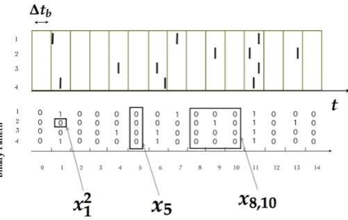
the time index of the measurements, denoted by∆tb1. Denoting the time index by the integer variable 109
t, one can say thatxkt =1 whenever thek-th neuron emits a spike during thet-th time bin, whilexkt =0 110
otherwise. This standard procedure transforms experimental data into sequences of binary patterns 111
(see figure1). 112
Aspike patternis the spike-state of all the measured neurons at time bint, which is denoted by 113
xt := xkt
N
k=1. Aspike blockis a consecutive sequence of spike patterns, denoted byxt,r :=
xsrs=t. 114
While the length of the spike blockxt,risr−t+1, is also useful to consider spike blocks of infinite 115
length starting from timet=0, which are denoted byx. Finally, is this paper we consider that aspike
116
trainis either a spike block of finite length or an infinite sequence of spiking patterns, which will be 117
useful later when discussing asymptotic properties. The set of all possible spike blocks of lengthR
118
corresponding to a network ofNneurons is denoted byAN
R. The set of all spike blocks of infinite 119
length is denoted byΩ≡ AN
N, which is a useful mathematical object as clarified below. Let us define
120
projR:Ω→ ANR the natural projection given byprojR(x) =x0,R−1.
121
2.2. Features
122
Following the machine-learning nomenclature, afeatureis a function that extracts a property of interest from the data. Formally, afeatureis defined as a function f :Ω →Rthat associates a real
number to eachx∈Ω. The feature f is said to have a temporal range or simply a rangeRif for every x,y ∈ Ωsuch thatx 6= y, one has that f(x) = f(y)if and only ifx0,R−1 =y0,R−1, that is, if f only
1 When binning, sometimes can be useful to go beyond the refractory period. In those cases, two spikes may occur within the
Figure 1.(Top) Each bar indicates a spike of a neuron indexed from 1 to 4 in continuous time. (Bottom) After binning∆tbthe spiking activity is transformed into binary patterns in discrete time. We illustrate
the notation used throughout this paper.
depends on the firstRspike patterns of the spike-train. A special class of features, over which this work is focused on, are binary functions consisting of finite products of spike states, i.e.
fl(x) = q
∏
k=1 xik
tk.
Above, l is a shorthand notation for the set{tk,ik}qk=1, where[tk]qk=1 and[ik]qk=1 are collections of time and neuron indexes respectively, and q is the number of spikes considered by the feature. Correspondingly, for a given indexl, one has fl(x) =1 if and only if theik-th neuron spikes at time
tk, for allk∈ {1, . . . ,q}in the spike-trainx, while fl(x) =0 otherwise. Note that, when considering features of rangeR ≥ 1, the firing timestk are constrained within the interval{0, . . . ,R−1}. We define the reduced feature ˜f :AR
N→Rsuch that
˜
f(x0,R−1) = f˜(projR(x)) = f(x).
2.3. Statistical structure
123
For a given spiking neuronal network involved in a particular experimental protocol, the 124
measured activity usually contains a significant amount of stochasticity that is characteristic of 125
measurements at this spatiotemporal scale. This randomness is caused mostly by 126
(i) the random variation in the ionic flux of charges crossing the cellular membrane per unit time at 127
the post synaptic button due to the binding of neurotransmitter, 128
(ii) the fluctuations in the current resulting from the large number of opening and closing of ion 129
channels [34,35], 130
(iii) noise coming from electrical synapses [36]. 131
the stationary assumption, given the probability distribution of the whole processp{·}one can define a unique corresponding probability distribution overAN
R following the natural projection, given by:
pR{B∈ ANR}:=p{proj−R1(B)∈Ω}. (1) As a consequence of assuming an stochastic process guiding the neuronal activity, a feature f :Ω→R
becomes a random variable. Consequently, the statistics of f are defined by
p{f =a}=p{x∈Ω|f(x) =a}.
In particular, considering the feature f(x) =xkt, one can note that individual spike-states (as well as spike patterns and spike blocks) become discrete random variables. As a convention, we denoteXk
t a random spike-state that follows an implicit underlying probability distributionp{·}, while lower-case expressions (e.g.xkt) are used for denoting concrete realization of these random variables. The mean value of a feature f with respect to the probabilityp{·}is given by:
Ep{f}=
∑
x∈Ωf(x)p{x}.
For the case of features of rangeR, the mean value can be expressed alternatively as:
Ep{f}=
∑
x0,R−1∈ANR˜
f(x0,R−1)pR{x0,R−1}=EpR
˜
f
which is a finite sum. Above, ˜f is the reduced feature, as defined in (2.2). 132
2.4. Empirical averages
133
Let us consider spiking data of the formx0,T−1, whereTis the sample length. Although in general
the underlying probability measurep{·}that govern the spiking activity is unknown, it is useful to use the available data to estimate the mean values of specific features. Iff is a feature of rangeR, the empirical average value of f from the samplex0,T−1is
AT(f) = 1
T−R+1 T−R
∑
i=0
f(xi,R−1+i). (2)
In particular, for features of range one, the previous expression becomesAT(f) = T1∑T
−1
i=0 f(xi). 134
An interesting questions is under which conditionsAT(f)→Ep{f}asTgrows. This, and other 135
convergence issues, are explored in Section4. 136
3. Inference of the statistical model with the MEP 137
138
Following Section2.3, the probability measurep{·}represents the inherent stochasticity of the 139
spiking neural population under consideration. Asp{·}is unknown, one would like to infer it from 140
data. In the sequel, we first introduce the general MEP as a method for inferringp{·}. Then, we show 141
this principle for the case where only synchronous constraints are considered, and finally, we present 142
the case of where non-synchronous correlations are included to constrain the maximization problem. 143
3.1. Fundamentals of the MEP
144
The MEP was first proposed by E. T. Jaynes as a way for estimating probability distributions when 145
the information for performing the inference is scarce [37]. Rooted in principles of statistical physics, 146
this approach selects a probability measure that satisfies the evidence supported by the available 147
randomness, Jaynes shows that the most natural metric is the Shannon entropy [38]. The probability 149
measure found by this procedure is known as themaximum entropy distribution. 150
Formally, the MEP is a concave constrained maximization problem, where the constraints that 151
define the optimization space correspond to the available information that guide the inference process. 152
Accordingly, if additional constraints are introduced then the optimization space is reduced; this 153
corresponds to the informative power of new information, which restricts the space of models that are 154
consistent with it. 155
The inference procedure based on the MEP follows the following steps: 156
I. ChooseKfeatures of interest f1, . . . ,fK(c.f. Section2.2). 157
II. Using the available datax0,T−1, compute the empirical averange of each featureAT(fk):=ck. 158
III. Assuming stationarity, define the space of statistical modelsM(c1, . . . ,cK)⊂ Mgiven by
M(c1, . . . ,cK) ={g∈ M|Eg{f1}=c1, . . . ,Eg{fK}=cK},
where Mis the set of probability measures and M(c1, . . . ,cK) is the family of probability 159
measures that are consistent with the empirical mean valuesc1, . . . ,cKobtained in Step II. 160
IV. Defining the entropy rate of the stochastic process as
S {p}= lim t→∞
1
t
∑
x0,t−1∈ANt
pt{x0,t−1}log
1
pt{x0,t−1}
, (3)
find the maximum entropy process, characterized by the probability measure
ˆ
p= arg max
q∈ M(c1,...,ck)
S {q}. (4)
Some small remarks are to be said about this procedure. One can think of this as a data-driven 161
algorithm, whose input is the datax0,T−1and output is the maximum entropy measure ˆp. The first two
162
steps of the process are known in the machine learning literature as "feature selection" and "feature 163
extraction", respectively (see e.g. [39,40]). The goal of these steps is to reduce the dimensionality of the 164
input for the subsequent stages, in order to prevent the selected model to overfitting the data (i.e. to 165
include in the model effects of noise and biases due to the finiteness of the data). Hence, what drives 166
the model selection stages is not the whole data but the quantitiesc1, . . . ,cK, which define the space to 167
be explored in Step 4. 168
Steps 3 and 4 are known as "model selection". According to the the machine learning jargon these 169
steps deliver a generative model, in the sense the obtained model can later be used to generate new 170
data. In this sense, it is interesting that although the data is finite, the entropy rate calculated in Step 4 171
is computed over all spike blocks of all lengthst, which is possible due to the generative nature of the 172
candidate models. The inputs for the model selection stages are not the whole datax0,T−1but only the
173
valuesc1, . . . ,cK, which represent the knowledge obtained from the data that guides the search in the 174
space of candidate models. Moreover, as these quantities represent all the available knowledge one 175
has about the underlying stochastic process generating the spikes, therefore, one would like to select a 176
model that reflect that information while making no further assumptions. By recalling the work made 177
by Claude Shannon on the analysis of information sources (c.f. [41] and references therein), one can 178
interpret the entropy rate as a measure of how hard is to predict the realization of a stochastic process. 179
This implies, in turn, that the maximum entropy measure withinM{c1, . . . ,cK}is the most random, 180
i.e unstructured, among those which satisfies the constraintsAT(f1) =c1, . . . ,AT(fK) =ck. Although 181
the framework presented above is general enough to encompass the cases when considering only 182
synchronous constraints and when considering also non-synchronous constraints, the methods used 183
the maximum entropy measure when only synchronous features are selected, leaving for section3.2
185
the more general situation including non-synchronous constraints. 186
3.2. Time-independent constraints
187
Assuming only synchronous interactions is equivalent to only consider features of range one (i.e. 188
features that consider neurons at the same time index, c.f. Section2.2), which leads to restricting the 189
candidate models to those in where the present state is statistically independent of past and future 190
states. Moreover, by the assumption of stationarity, this leads to modeling the collective spiking activity 191
as a sequence of i.i.d. random variables. The challenge, in this case, is to estimate the corresponding 192
distribution as reliably as possible. A large portion of the literature of maximum entropy spike train 193
statistics focus on synchronous interactions between neurons, implicitly neglecting interactions across 194
time. Although this assumption induces a strong simplification, the resulting models have proved to 195
be rich in structure and can provide interesting results and insights about the neural code [6,12]. In 196
the following, we recall how this problem can be addressed using the MEP. 197
As a consequence of the assumptions of temporal independence and stationarity, it can be shown that (4) is reduced to
ˆ
p1= arg max
q1∈ M1(c1,...,ck)
∑
x0∈A1Nq1{x0}log
1
q1{x0}
(5)
whereM1(c1, . . . ,ck)corresponds to the set of distributionsq1overA1N(c.f. range one projections in
(1)) such that the constraintsEq1{fk}=ckare satisfied for eachk=1, . . . ,K. Note that the above sum is over the 2Npossible spike patterns, being a simpler condition than (4). In fact, following a simple argument based on Lagrange multipliers and the concavity of the entropy, it can be show that the distribution ˆp1that solves (5) is unique. Moreover, is a Boltzmann-Gibbs distribution [38]:
ˆ
p1{x0}= e −Hβ(x0)
Z(β) ∀x0∈ A N
1; Z(β) =
∑
x0∈AN1
e−Hβ(x0), (6)
whereHβis referred as theenergy or potentialfunction 198
Hβ(x0) =
K
∑
k=1
βkf˜k(x0), (7)
β∈RKis the vector of Lagrange multipliers. Following the statistical physics literatureZ(β)is called 199
thepartition function, whose logarithm is referred asfree energy. 200
Conversely, from the uniqueness property of the maximum entropy distribution one can conclude that there is only one Boltzman-Gibbs distribution ˆp1that belongs toM(c1, . . . ,cK), being the only solution of (5). Interestingly, this alternative approach is much easier to solve the original optimization problem2. In effect, one only need to find the values of the parameter vectorβkthat reproduces the empirical average valuesc1, . . . ,cK. Moreover, it is known that for any Boltzmann-Gibbs distribution
p1the following holds:
∂lnZ(β)
∂βk
=Epˆ1(f˜k). (8)
Therefore, using (8) one could find the appropriate values ofβfor whichEpˆ1{f˜k}=ckare satisfied 3.
201
2 In particular,M
1{c1, . . . ,ck}is not easy to parametrize and hence the application of standard techniques of convex
optimization (e.g. gradient decent) is not straightforward.
3 However, for practical purposes this problem cannot be solved for systems withN>20 [8], so alternative procedures are
3.3. Non-synchronous constraints
202
A generalization of the previous approach is to include average values of features corresponding to interactions in the spiking activity across time as constraints. This is a natural assumption in biological spiking networks as it is expected that the spike of one neuron influence other subsequent spikes. Statistical models with time-dependencies can be generated with the MEP by introducing features that involve different time indexes. In effect, selecting features of rangeRinduces interdependencies and a corresponding "memory" in the model of lengthR−1, and thus it is natural to look for the best suited Markov chain over the state spaceAR
N. A Markov chain model would allow to express the probability of a spike trainx0,TforT>Ras
p{x0,T}=π{x0,R−1}P{x1,R|x0,R−1} · · ·P{xT−R,T−1|xT−R+1,T},
wherePis a transition probability matrix4andπis a corresponding invariant probability distribution
203
(which is unique due to the ergodicity assumption, c.f. Section3.3.1) associated toP. Note that, due to 204
the stationarity condition, the transition probabilitiesP{·|·}are constant over the realization of the 205
whole process (see AppendixAfor more details.). 206
Following the MEP as described in Section3.1, we look for a procedure for finding a Markov transition matrixPthat maximizes its entropy rate while satisfying some constrains given the empirical averages of observables f1, . . . ,fK. For ergodic Markov chains, a well-known calculation (that can be found e.g. in [41]) shows that the entropy rate, as given by (3), is equivalent to the following simple expression:
SKS(π,P) =−
∑
i,j∈AR N
πi
∑
jPijlogPij. (9)
whereπi=π{x0,R−1=i}andPij =P{j|i}fori,j∈ ANR. Is important to notice that (9) corresponds 207
to theKolmogorov-Sinai entropy (KSE)in the dynamical systems literature [44]. In general (9) is larger 208
when for a fixedithe conditional probabilitiesPij are closer to an uniform distribution, i.e. when 209
knowing the transition statistics gives little certainty about the next step. 210
It can be shown that, if the considered features do not involve correlations across time (i.e. they 211
are features of range 1, c.f. Section2.2), then the resulting transition probabilities are such that the 212
corresponding stochastic process is i.i.d (i.e. whenPij=πj). Interestingly, in this scenario equation 213
(9) reduces to the Shannon entropy ofπi. This clarifies that this approach based on Markov chains
214
extends the classical MEP and the results presented in Section3.2. 215
Finding the MEMC raises, however, some extra technicalities with respect to the time-independent 216
case. Recall that the goal is no longer to estimate a probability distribution, but to reconstruct from 217
data a transition matrixPand a corresponding invariant measureπ. The challenge is that asPandπ
218
are not independent parameters of the process (πhas to be the eigenvector associated with the unitary
219
eigenvalue ofP[45]), therefore one cannot apply Lagrange multipliers over the entropy rate function 220
(9). In the sequel we explore an alternative route to build the MEMC based on the transfer matrix 221
technique. This technique is computationally simple, and also provides further insightful connections 222
with statistical physics and thermodynamics. 223
3.3.1. Transfer Matrix Method 224
In order to find the MEMC associated with non-synchronous constraints, we follow the same 225
ideas presented above in the time-independent case, but using different tools. We present them here. 226
Let us consider the set of features chosen to constrain the maximization of entropy rate (step I in 227
3.1). We assume that the features chosen have a finite maximum rangeR. From these features one can 228
4 Note thatP{·,·}has a consistency requirement: forw,y∈ AR
build the energy functionHβ(7) of finite rangeRas a linear combination of these features. Using this 229
energy function we build a matrix denoted byLHβ, so that for everyy,w∈ ARNits entries are given as
230
follows: 231
LHβ(y,w) =
(
eHβ(ywR−1) ify
1,R−1=w0,R−2
0, otherwise. (10)
ByywR−1we mean the word obtained by concatenation ofy1andw1,R−1. In the particular case of
232
energy functions associated to range one features, we the aboves matrix is defined asLHβ(y,w) =
233
eHβ(y). AssumingH
β >−∞, the elements of the matrixLHβ are non-negative, this in turn implies 234
ergodicity. Moreover, the matrix is primitive by construction, thus it satisfies the Perron-Frobenius 235
theorem [46]. Hereafter LH will be referred as the Ruelle-Perron-Frobenius matrix (RPF). Let us
236
denote beρthe largest eigenvalue ofLH, which because it satisfies the Perron-Frobenius theorem is an
237
eigenvalue of multiplicity one and strictly larger in modulus than the rest of the eigenvalues [46]. We 238
denote byUandVleft and right eigenvectors ofLHβ corresponding to the eigenvalueρ. Notice that
239
Ui >0 andVi>0, for alli∈ ANR. 240
The RPF matrix is not the Markov matrix we are looking for, moreover, is not a stochastic matrix, 241
but can be converted into a stochastic matrix. We recall that for an irreducible matrixMwith spectral 242
radiusλ, and positive right eigenvectorvassociated toλ, then thestochasticizationofMis the following
243
stochastic matrix: 244
S(M) = 1
λD
−1MD, (11)
whereDis the diagonal matrix with diagonal entriesD(i,i) = vi. So, in our context, the MEMC transition matrix is given as follows:
P=S(LHβ), (12)
whose unique stationary probability measureπis explicitly given by
πi:= hUUiVi
,Vi, ∀i∈ A
N
R, (13)
wherehU,Viis the standard inner product inRNR(we refer the reader to [46] for details and proofs).
245
3.3.2. Thermodynamic formalism 246
In the previous section we have shown how to obtain the transition matrix and the invariant 247
measure of a Markov chain. However, we have not yet included the constraints (we have just used the 248
features to build the energy function), in other words, we have not yet fit the parameters of the MEMC. 249
In order to fit the maximum entropy parameters let us introduce the following quantity, 250
P
Hβ
= sup q∈Mst
n
S {q} + EqHβ
o
(14)
whereMstis the set of all stationary probability measures inARNandEqHβ =∑ K
k=1βkEq{fk}is 251
the average value ofHβwith respect toq. Solving the optimization problem (14) one gets the Markov 252
measure we are looking for. Indeed, one knows from the thermodynamical formalism (see [47]) that 253
for our energy functionHβof rangeR≥2, there exists an unique translation invariant (stationary) 254
Markov measurepassociated toHβfor which one has the constantM>1 such that, 255
M−1≤ p{x1,n}
exp(∑nk=−1R+1H(xk,k+R−1)−(n+R−1)P[Hβ])
that attains the supremum (14), that isS {p} + EpHβ . The quantityP[Hβ] is calledtopological 256
pressure, which plays the role of the free energy in the statistical mechanics. The measurep, as defined 257
by (15), is known as the Gibbs measure in the sense of Bowen. Note that one can show that MEMCs 258
are particular cases of these measures, associated to finite-range energy functions. Moreover, (6) is a 259
particular case of (15), whenM=1 andHβis an energy function of range one. 260
The average values of the features, their correlations, as well as their higher cumulants can be obtained by taking the successive derivatives of the topological pressure with respect to their conjugate parametersβ. This explains the important role played by the topological pressure in this framework. In general,
∂nPHβ
∂βnk =κn ∀k∈ {1, ...,K}, (16)
whereκnis the cumulant of ordern(see appendixB.). In particular, taking the first derivative: 261
∂PHβ
∂βk
=Ep{fk}=ck, ∀k∈ {1, ...,K}, (17)
whereEp{f}is the the average of fkwith respect top(maximum entropy measure), which is equal 262
(by assumption) to the average value of fkwith respect to the empirical measure from the datack, that 263
constraint of the maximization problem. These equations suggest a relationship with the logarithm 264
of the free energy or log partition function of the Boltzmann Gibbs distribution. Indeed, for range 265
one potentials (time-independent Maximum entropy distributions)ρ(β) =Z(β)andP[Hβ] =lnZ(β) 266
which relates (8) with (17) (For a detailed example see section5.2). This problem of estimating the 267
MEMC parameters become computationally expensive for big matrices. However, there exist efficient 268
algorithms to estimate the parameters for the Markov maximum entropy problem in the literature [42]. 269
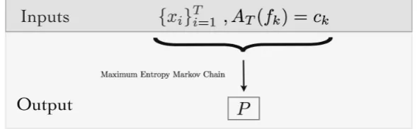
Figure 2.Algorithmic view of the MEMC: Inputs are the spike trains{xi}Ti=1and the average values of
a set of features. The output is the MEMC transition matrixP
4. Large deviations and applications in MEMC 270
4.1. Preliminary considerations
271
This subsection reviews two elementary tools for studying the convergence of random variables 272
while providing corresponding references. In the sequel, first the central limit theorem is introduced in 273
subsection4.1.1, and then large deviation theory is discussed in subsection4.1.2. 274
4.1.1. Central limit theorem 275
Let us first assume that one can have access to arbitrarily large data sequences. Considert∈N
276
and letx0,t−1be the spike-block of lengtht(which is allowed to increase), and let f :Ω →Rbe an
277
arbitrary feature (not necessarily belonging to the set of features chosen to fit the MEMC). In this 278
section we establish asymptotic properties ofAt(f)sampled with respect to the MEMC characterized 279
Through this work, we will assume thatp{·}is an ergodic Markov probability measure, this meaning that every spiking block inAN
R is attainable from every other block in the Markov chain withinRtime steps as discussed in section3. Thanks to the ergodic assumption, it is guaranteed that the empirical averages become statistically more accurate as the sampling size grows [48], i.e.,
At(f)→Ep{f}.
However, the above result does not clarifies the rate at which the estimate accuracy improves. For 281
answering this question, one can use the central limit theorem (CLT) for ergodic Markov chains (see 282
[49]). This theorem states that there exists a constantσ>0 such that for large values oft, the random
283
variable
√
t σ
At(f)−E{f}distributes as a standard Gaussian random variable5, withσbeing the
284
square-root of the auto-covariance function off [49]. This, in turn, implies that “typical” fluctuations 285
ofAt(f)around its mean valueE{f}are of the order ofσ/
√ t. 286
4.1.2. Large deviations 287
Although the central limit theorem for ergodic Markov chains is accurate in describing typical events (which are fluctuations around the mean value), it does not say anything about the likelihood of larger fluctuations. Despite that it is clear that the probability of such large fluctuations goes to zero as the sample size increases, it is valuable to describe the corresponding decrease rate. In particular, one says that an empirical averageAt(f)satisfies a large deviation principle (LDP) with rate function
If, defined as
If(s):=−lim t→∞
1
t logp{At(f)>s}, (18)
if the above limit exists. Intuitively, the above condition for largetimplies thatp{At(f)>s} ≈e−tIf(s). 288
In particular, ifs>Ep{f}the Law of Large Numbers (LLN) guarantees thatp{At(f)>s}tends to 289
zero astgrows; the rate function quantifies the speed at which this happens. 290
CalculatingIf directly, i.e. by using the definition (eq18), can be a formidable task. However, the Gärtner-Ellis theorem provides a smart shortcut for avoiding this problem [24]. To this end, let us introduce thescaled cumulant generating function(SCGF)6associated to the random variablef, by
λf(k) =: lim t→∞
1
t lnEp
h
etkAt(f)i, k∈R, (19)
when the limit exists (further general details about cumulant generating functions are found in 291
AppendixB). Note that, whileAt(f)is an empirical average taken over a sample, the expectation 292
in (19) is taken over the probability distribution given by the corresponding model p{·}. If λf is
293
differentiable, then the Gärtner-Ellis theorem ensures that the averageAt(f)satisfies a LDP with rate 294
function given by the Legendre transform ofλf, that is 295
If(s) =max k∈R
{ks−λf(k)}. (20)
Therefore, in summary, one can study the large deviations of empirical averages At(f) by first 296
computing their SCGF from the selected model and then finding their Legendere transform. 297
5 Technically, the central limit theorem says that
p
(√
t σ
At(f)−E{f}≤x
)
→ √1
2πσ
Z x
−∞e
−s2
2σds,
where the convergence is in distribution.
6 The name comes from the fact that then-th cumulant offcan be obtained bytsuccessive differentiation operations over of
One of the most useful applications of the LDP is to estimate the likelihood thatAt(f)adopts a value far from its expected value. For illustrate this, let us assume thatIf(s)is a positive differentiable convex function7. Then, because of the properties of convex functions If(s)has a unique global minimum. Denoting this minimum bys∗, it follows from the differentiability ofIf(s)thatIf(s∗) =0, and using properties of the Legendre transforms∗ = λ0f(0) = limt→∞Ep(f). This is the LLN, i.e.,
At(f)gets concentrated arounds∗. Consider a values 6=s∗and assume thatIf(s)admits a Taylor series arounds∗given by
If(s) =If(s∗) +I0f(s
∗
)(s−s∗) + I 00
f(s∗)(s−s∗)2
2 +O(s−s
∗ )3
Sinces∗must correspond to a zero and a minimum ofI(s), the first two terms in this series vanish, 298
and asI(s)is convex functionI00(s)>0. For large values ofk, we obtain from (18) 299
p{At(f)>s} ≈e−tIf(s)
≈e −t I
00
f(s∗)(s−s∗)2
2
!
(21)
so the small deviations of At(f)arounds∗are Gaussian-distributed as for i.i.d. sums 1/I00f(s∗) = 300
λ00f(0) =σ2. In this sense, large deviation theory can be seen as an extension of the CLT because it
301
gives information not only about the small deviations arounds∗but also about large deviations (not 302
Gaussian) ofAt(f). 303
4.2. Large deviations for features of MEMC
304
In this section, we focus on the statistical properties of features sampled from the inferred MEMC. 305
For example, one may be interested in measuring the probability of obtaining "rare" average values of 306
features like firing rates, pairwise correlations, triplets or spatiotemporal events. This characterization 307
is relevant as these features are likely to play an important role in neuronal information processing, and 308
rare values may hinder the whole enterprise of conveying information. We show in this section how to 309
obtain the large deviations rate functions of arbitrary features through the Gärtner-Ellis theorem via 310
the SCGF. In particular, we show that the SCGF can be directly obtained from the inferred Markov 311
transition matrixP. 312
Consider MEMC taking values on the state spaceAN
R with transition matrixP. Let f be a feature 313
of rangeRwhich consider only the block andk∈R, we introducePe(f)(k), thetilted transition matrix by
314
f ofP, parametrized byk, whose elements are given by: 315
e
Pij(f)(k) =Pijek f(j) i,j∈ ANR. (22) For transition matricesPinferred from the MEP, the tilted transition matrix can be built directly 316
from the spectral properties of the transfer matrix (10) as follows, 317
e
Pij(f)(k) = e Hβ(i,j)V
j
Viρ e
k f(j) (23)
= e
[Hβ(i,j)+k f(j)]V
j
Viρ i,j∈ A
N R.
7 A classical result in LDP states thatI
f(s)is a convex function ifλf(k)is differentiable [25]. For a discussion about the
Recall thatVis the right eigenvector of the transfer matrixL. Here we also have used the shortcut 318
notationHβ(i,j)to indicate that the energy function takes the contributions from the blocksiandj. 319
Remarkably, the feature f does not need to belong to the set of chosen features to fit the MEMC. 320
Now, we can take advantage of the structure of the given process in order to obtain more explicit 321
expressions for the SCGFλf(k), for instance, if one considers i.i.d. random variablesXthen, from the 322
very definition one can obtain that 323
λ(k) = lim
t→∞
1
tlnE[e
kX]t=ln
E[ekX],
which is the case of range one features. So, using equation (22), we get that the maximum eigenvalue 324
of the tilted matrix, denoted byρ(Pef(k))is,
325
ρ Pef(k)
=
∑
j
πjek f(j) j∈ AN1.
SincePef is a positive matrix the Perron-Frobenius theorem ensures the uniqueness ofρ.
326
Next, for the case of additive features, one deals with positive Markov chains, and under the assumption of ergodicity, an straightforward calculation (see for instance [51]) leads us to obtain that
λf(k) =ln ρ Pe(f)
. (24)
It also can be proved thatλf(k), in this case is differentiable [51], setting up the scene to apply the
327
Gärtner-Ellis theorem, which bypasses the direct calculation ofp{AT(f)>s}in (18), i.e., havingλf(k), 328
its Legendre transform leads to the rate function of f as shown in figure3. 329
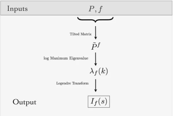
Figure 3.Algorithmic view of the method: Inputs are the maximum entropy Markov transition matrix and a feature. From the inputs the tilted transition matrix can be built. The rate function of the feature is obtained as the Legendre transform of the log maximum eigenvalue of the tilted transition matrix. Using this framework we can estimate the large deviations of the average values of the features.
4.3. Large deviations for the entropy production
330
A stochastic process is said to be in equilibrium if one cannot notice the effect of time on it. It is 331
worth noticing that non-equilibrium stochastic processes are natural candidates to model spike train 332
rangeR>1 as constraints in the maximum entropy problem is that it opens the possibility to break 334
the time-reversal symmetry present in the time-independent models. This captures the irreversible 335
character of the underlying biological process and thus, allows to fit more realistic statistical models 336
from the biological point of view. 337
To characterize this mathematically, we study how the distributionp{·}changes when the time 338
order is reversed. For this aim, let us consider a spike blockx0,T−1 = x0,x1, . . . ,xT−1containingT
339
spike patterns, and define the time-reversed spike blockx0,(RT)−1obtained by re-ordering the time index 340
in reverse order, i.e.,x(0,RT)=xT−1,xT−2, . . . ,x2,x0.
341
A spiking network modeled byp{·}is said to be in equilibrium ifp{x0,T}= p{x(0,RT)}for allx [52]. For a homogeneous discrete time ergodic Markov chain characterized by the Markov measure
p(π,P)taking values inANR, to be in equilibrium is equivalent to satisfy thedetailed balance conditions,
which is given by the following set of equalities:
πiPij=πjPji, ∀i,j∈ ANR.
Conversely, when these conditions are not satisfied the statistical model of the spiking activity is said to be a non-equilibrium system. Since non-equilibrium is expected to occur generically in neuronal network models, one would like to quantify how far from equilibrium is the inferred MEMC. For this purpose one can define theinformation entropy production(IEP) forp, which is given by
IEP(p):= lim t→∞
1
t ln
"
p{x0,t−1} p{x(0,Rt)−1}
#
,
when the limit exists. For the maximum entropy Markov measurep(π,P), the IEP is explicitly given
by:
IEP(π,P) = 1
2i,j
∑
∈AN R
πiPij−πjPji
logπiPij
πjPji
, (25)
(see [53] for the calculation). We remark that it is still possible to obtain the information entropy 342
production rate also in the non-stationary case. Clearly, for features of range one, IEP = 0 343
always, meaning that the process is time-reversible, therefore the probabilities of every path and 344
its corresponding time-reversal path are equal. For features of rangeR>1,IEP>0 generically (we 345
refer the interested reader to [22] for details and examples). 346
However, since in practice one only have access to limited amount of data, a natural question is to ask for the entropy production of the system considered up to a finite amount of time. It turns out that this characterization can be obtained through a LDP. With this in mind one may define the following feature:
WT(x0,T−1) = 1 Tln
"
p(x0,T−1) p(x(0,RT)−1)
#
.
Since we have assumed that samples are produced by a stationary ergodic Markov chain characterized byp(π,P), the ergodic theorem assures that forp-almost every sample, the quantityWtwhentgoes to infinity converges, and it is by definition the IEP,
lim
Once we have the convergence forWt, we may ask for its large deviation properties. Under the same idea above, and following [54], we introduce the following matrix:
Fij=Pijln
"
πiPij
πjPji
#k
i,j∈ ANR,
this matrix help us to build the SCGF associated toWt, through the logarithm of the maximum 347
eigenvalueρF(k). Using the Gärtner-Ellis theorem one gets the rate functionIW(s)for the IEP. 348
4.4. Large deviations and MEMC distinguishability
349
It is clear that there exist a relationship between accuracy of the estimation and sample size. The larger the sample size the more information is available and the uncertainty diminish. In the context of maximum entropy models, this idea has been well conceptualized using tools from information geometry [27,55]. The main idea of this approach is that the maximum entropy models form a manifold of probability measures whose coordinates are the parametersβ. Consider a spike train datasetx0,T−1
consisting ofT spike patterns obtained from a spiking neuronal network. Given a set of features
{fk}Kk=1and their empirical averages, one may infer the parametersβ= (β1, . . . ,βK)characterizing
the MEMC p(π,P). We may use the inferred MEMC to generate a samplex00,T−1of the same size
as the original dataset. Considering the same set of features one may apply again the MEP to infer a new set of parametersβ0fromx00,T−1, which is, in general, expected to be different fromβ. These
maximum entropy models will belong to a certain volume in the manifold which will decrease as the sample size increase [27]. On the other hand, increasing the sample size ofx00,T−1, one expects that
the Markov chainp0(π0,P0)specified byβ0 gets "closer" to the one characterized byβ. The idea of relating a distance in the parameter space with a distance in the space of probability measures can be rigorously formulated using large deviations techniques. Let us start by defining the relative entropy between these two MEMC (Gibbs measures in the sense of Bowen (15)), which provides a notion of "distance"8. In order to do that in the context of MEMC’s consider a Gibbs measurepassociated to the energy functionHβ, and letqbe another Gibbs measure. The Ruelle-Föllmer theorem gives us an expression for the relative entropy density between two Gibbs measures in terms of the pressure, the entropy rate and the expected value of the energy function with respect toq(see [26]), as follows:
d(q| p) =P[Hβ]−S(q)−Eq(Hβ). (26)
Observe that ifd(q| p) =0, we obtain the variational characterization of Gibbs measures (14). 350
Consider the potentialHβ=∑ K
k=1βkfkassociated with a MEMCp(π,P). Given a set of empirical
351
averagesAt(fk)generated by a sample ofp(π,P)we obtain new maximum entropy parametersβ0. 352
The probability that the maximum entropy parametersβ0associated with an ergodic Markov Chain 353
p0(π0,P0)get close toβfollow the following large deviation principle [25]: 354
lim δ→0
lim t→∞
−1
t lnP
| β−β0|∈∆δ
=d(p| p0), (27)
where∆δ= [−δ,δ]K. Calling and the vectorδβ= β−β0and choosing∆δclose to 0 we informally 355
rewrite the above corollary in the form: 356
−1
t lnP
|δβ|∈∆δ
−→
t→∞d(p|p
0)
. (28)
Thus, for largeTwe get: 357
P
|δβ|∈∆δ
≈e−td(p|p0),
which implies that close-by parameters are associated to close-by probability measures [27]. 358
Consider now two MEMCp(π,P)andp0(π0,P0)specified byHβandHβ0respectively with the 359
same family of features. We say that the MEMC’s aree-indistinguishableif:
360
−lnP
|δβ|∈∆δ
≤e. (29)
As both MEMC’s satisfy the variational principle (14), the relative entropy betweenpandp0(26) reads: 361
d(p| p0) =P[Hβ0]− P[Hβ] +p(Hβ)−p(Hβ0). (30)
Taking the Taylor expansion ofd(p| p0)aroundβ0=βwe get: 362
d(p| p0)≈d(p| p) +
∑
k
∂d(p|p0) ∂β0k
β0=β
(βk−β0k) + 1
2
∑
k,j∂2d(p| p0) ∂β0kβ0j
β0=β
(βk−β0k)(βj−β0j).
Sinced(p| p0)is minimized atβ0 =βwe obtain,
363
d(p|p0)≈ 1
2
∑
k,j∂2d(p| p0) ∂β0kβ0j
β0=β
(βk−β0k)(βj−β0j).
Taking the second derivative ofd(p| p0)from (30), one also has that, 364
∂2d(p|p0) ∂β0kβ0j =
∂2P[Hβ0]
∂β0kβ0j =Lkj. (31)
The second partial derivatives of the topological pressure with respect to the parametersβ0kandβ0jcan
365
be conveniently arranged in a matrixLwith componentsLkj. Given two MEMC’s specified byHβand 366
Hβ0, in the limit of largetthey aree-indistinguishable if:
367
1 2
h
(δβ)TL(δβ)
i
≤ e
T, (32)
whereTdenotes transpose. The matrixLcan be obtained from data without need to fit the parameters. 368
Equation (32) characterize a region in the space of MEMC of indistinguishable models, whose 369
volume can be calculated in the largetlimit using spectral properties of the matrixL[27]. This result 370
generalizes a previous result for maximum entropy distributions for range one energy functions in [28]. 371
372
5. Illustrative examples 373
In this section we illustrate the presented methods in some simple scenarios. In these examples 374
we follow a set of steps: 375
1. Choose the features and build the energy function (7). 376
2. Build the transfer matrix (10). 377
3. Compute the free energy and find the maximum entropy parameters using (17). 378
4. Build the Markov transition matrix using (12). 379
5. Choose the observable to examine and build the tilted transition matrix using (22). 380
6. Compute the Legendre transform of the log maximum eigenvalue of the tilted transition matrix 381
to obtain the rate function (24). 382
For the sake of clarity, in this section we focus on small neuronal networks. It is clear, however, 383
5.1. First example: Maximum entropy model of a range 2 feature
385
Consider spiking data from two interacting neurons. We measure only the average value of 386
a of a range 2 feature from the spiking data to fit a MEMC. The feature denoted by f1is given by
387 ˜
f1(x0,1) =x20·x11, which detects when a spike of the second neuron is followed by a spike in the first
388
one. The system can be described with the help of an energy functionH(x0,1) =β1f1˜(x0,1).
389
For a given dataset ofTspike blocks of range 2 the empirical average reads, 390
AT(f1) =c (33)
this means that in the data one finds that this event appearsc% of the time. 391
The transfer matrixLH(c.f. (10)) is primitive by construction (c.f. (10)), it satisfies the hypothesis
of the Perron-Frobenius theorem. In fact, its unique maximum eigenvalue isρ(β1) =eβ1+3. Given
the restriction (33), using (17) we obtain the following relationship between the parameterβ1and the
value of the restrictionc:
∂P[H] ∂β1
= ∂log(e β1+3)
∂β1
= e
β1
eβ1+3 =c.
This equation can be solved numerically. Using the obtained value of β1in equation (12) one can
392
find the corresponding Markov transition matrix. Note that, among all the Markov chains that match 393
exactly the restriction, the selected one maximizes the KSE. Moreover, it is direct to check that the 394
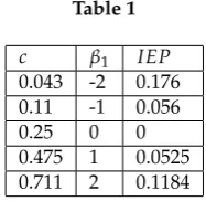
variational principle (14) is satisfied. Examples of values ofβ1for different values ofcand IEP (25) for
395
each value ofβ1are given in the following table:
396
Table 1
c β1 IEP
0.043 -2 0.176 0.11 -1 0.056
0.25 0 0
0.475 1 0.0525 0.711 2 0.1184
Having the MEMC, we are now interested in analyzing the statistical fluctuations of the feature f1. 397
Using equation (22) we obtain the tilted transition matrixPe
(f1)
ij (k)for each of the values in the table 398
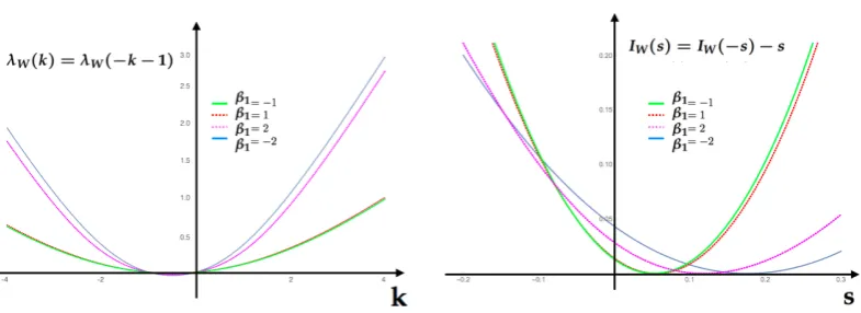
1. In figure (4), we compute for each value ofβ1we compute the SCGFλf1(k)(24) and the Legendre
399
transform (rate function) associated to the featureIf1(s). In figure (5), we compute for each value of
Figure 4. A)SCGF (24) for the feature f1of the first example computed at the values provided by the
table above.B)Rate function for the same feature computed at the same parameter values as the SCGF. Each of this functions are obtained taking the Lagrange transform of the respective SCGF inA).
400
Figure 5.Gallavotti-Cohen symmetry relationship for the IEP for values in table 1. Left SCGFλW(k).
Right rate function of the IEP featureW,IW(s).
5.2. Second example: Maximum entropy model with only synchronous constrains
402
Let us now consider a network of three neurons. We focus here on range one features. In this example we consider features related to the firing rates and synchronous pairwise correlations (Ising model [6,7]). Specifically, we consider the following energy function:
H(x0) =β1x10+β2x02+β3x30+β4x10·x20+β5x10·x03+β6x20·x30,
with the six parametersβ1, . . . ,β6. Following (10), the transfer matrixLHindexed by the states ofA31
is the following:
LH=
1 eβ1 eβ2 eβ1+β2+β4 eβ3 eβ1+β3+β5 eβ2+β3+β6 eβ1+β2+β3+β4+β5+β6
..
. ... ... ... ... ... ... ...
1 eβ1 eβ2 eβ1+β2+β4 eβ3 eβ1+β3+β5 eβ2+β3+β6 eβ1+β2+β3+β4+β5+β6
·
This matrix is primitive, and the unique maximum eigenvalue is
ρ(β) =1+eβ1+eβ2+eβ1+β2+β4+eβ3+eβ1+β3+β5+eβ2+β3+β6+eβ1+β2+β3+β4+β5+β6.
The right eigenvector associated to this eigenvalue has all the components equal to 1. We obtain the 403
topological pressureP[H] =logρ(β). In order to find the MEMC parameters we solve this set of
404
equations: 405
∂P[H] ∂β1
=AT(fk) =ck. (34)
From equation (34) provided some constraints on the average value of the features we can solve 406
the maximum entropy problem. Take for example (see table 2): 407
Table 2
AT(fk) ck βk δβk c˜k
AT(x1) 0.3 -1.0436 0 0.30350016
AT(x2) 0.2 -1.6727 0 0.20127414
AT(x3) 0.1 -2.8163 0 0.10450018
AT(x1x2) 0.08 0.4590 0 0.08187418
AT(x1x3) 0.05 0.8604 0.1 0.05475019
From equation (12) one can find that the Markov transition matrix. In order to compute the rate 408
function of each feature in this model, we take the logarithm of the maximum eigenvalue of the tilted 409
matrix, and obtain the tilted cumulant generating functionλf(k). In figure6) we illustrate the rate 410
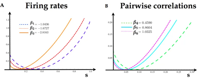
functions for each feature in the model. 411
Figure 6. A)Rate functions for the firing rates of each neuron of the Ising model. The minimum of the rate functions coincide with the expected value of the firing rates in the table 2.B)Rate functions for the pairwise interactions computed from the parameters in the table 2.
5.3. Third example: Past independent and Markov maximum entropy measures
412
For illustrating the difference between synchronous and non-synchronous maximum entropy models, we studied a simple model composed of two interacting neurons:
H(x0,1) =β1x10·x21+β2x02·x11+β3x01·x20. (35)
We build a Markov chain by fixing the parameters ofHatβ1=−3,β2=3,β3=0.5 in the state space
413
A2
1, given by
414
(
0 0
!
, 0
1
!
, 1
0
!
, 1
1
!)
.
whose corresponding transition matrix is given by
P=
0.13026 0.02580 0.65762 0.18632 0.65763 0.13026 0.16529 0.04682 0.02580 0.10266 0.13026 0.74128 0.15015 0.59735 0.03774 0.21476
.
We focus on the synchronous feature f = x10·x02, whose average value with respect to the Markov 415
measurepfixed by the parametersβ1,β2,β3isEp{x10·x20}=0.292611.
416
Using this particular Markov chain we generate a sample of sizeT=20.000. Then, we consider this data as a spike train of two neurons from which we have no other information. Starting from this data, we find the maximum entropy distribution that only considers the empirical average of the synchronous featureAT(x10·x20) =0.2926 as constraint. Therefore, we build a second model that uses
the following energy function:
˜
Using the constraint, we obtain from equation (8) ˜β = 0.215874 fixing the maximum entropy
417
distribution ˜p. Note that by constructionEp˜{x10·x20}= AT(x10·x20) =0.2926.
418
For both energy functions (35),(36) with the parameters mentioned before, we compute the rate 419
functions of the synchronous feature. Additionally, from the sample of the Markov chain given in (5.3) 420
we compute the empirical averages of the synchronous feature using sliding windows of 50 samples. 421
As expected, these empirical averages fluctuate around the overall average, as shown in Figure7. 422
Figure 7. A)Rate functions of the synchronous featurex10x20for both energy functions. B)Moving averages computed from a sample of length 20.000 of the Markov Chain with transition matrixP.
To test the relevance of including memory into the model (and assess the performance of 423
memoryless features), we compared the statistics of the fluctuations seen in the empirical average with 424
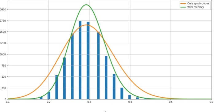
the prediction by the rate functions of the two models. Figure8shows the histogram of empirical 425
fluctuations, and plots the theoretical estimations of the fluctuations given byKexp{−W If(s)}, where 426
W=50 is the window size,sis the fluctuation size,If(s)is the rate function, andKis a constant that 427
is adapted for visualization purposes. 428
.
Figure 8.The fluctuations of the synchronous feature around the mean computed from the sample of the Markov chain are indicated with the bars. The Gaussian fluctuations around the mean predicted by the large deviations rate functions of both models are plotted. In green the curve predicted by the Markov model obtained fromHand in orange the curve predicted by the model obtained from ˜H
Results show that the rate function of the model with memory fits accurately the relative 429
the fluctuation’s frequencies, having a much larger variance that the data, and under estimates near 431
around the expected value. 432
6. Conclusion 433
In the past few years, new experimental techniques combined with clever ideas from statistical 434
mechanics have made possible to infer maximum entropy models of spike trains directly from 435
experimental recordings. However, a very important issue which is to quantify the accuracy of 436
the estimation obtained from a finite empirical sample is usually ignored in this field. This is probably 437
because the maximum entropy approach has a dual nature; one side is a convex optimization problem 438
which provides a unique solution independent of the sampling size, and on the other hand is a Bayesian 439
inference procedure, from which is more natural to ask this question. As we have discussed in the 440
introduction this characterization is relevant in the field of computational neuroscience as, in practice, 441
experimental recordings are performed during a finite amount of time which causes fluctuations over 442
the estimated quantities. 443
A fundamental goal of spike train analysis over networks of sensory neurons involves building 444
accurate statistical models that predict the response of the network to a stimulus of interest. In 445
particular, the aim of statistical inference of spiking neurons using the MEP, is that the fitted parameters 446
shed light on some aspects of the neuronal code, therefore it is extremely important to quantify the 447
accuracy of the statistical procedure. Additionally, one may be interested in measuring some properties 448
of the inferred statistical model characterizing the spiking neuronal network. For example about 449
convergence rate of a sample or to quantify the probability of rare events of features like firing rates, 450
pairwise correlations, triplets or spatiotemporal events, mainly because these features are likely to play 451
an important role in neuronal information processing. It is possible that rare and unlikely events have 452
been generated by internal states of the neuronal tissue and not driven by the external stimulus. The 453
events that are unlikely to occur deserve a better understanding as may carry important information 454
about the network internal structure and may play a role in organizing a coherent dynamic to convey 455
sensory information to the cerebral cortex. 456
The present contribution addressed this issue using tools from large deviations theory in the 457
context of the MEMC. In particular, we showed that the transfer matrix technique used to build the 458
MEMC is well adapted to compute large deviation rate functions using the Gärtner-Ellis theorem. We 459
also provide tools to investigate how sharply determined are the parameters of a MEMC with respect 460
to the amount of empirical data using the concept ofedistinguishability. Additionally, we present a
461
non-trivial relation between the distance in the parameter space and the distance in the manifold of 462
maximum entropy probability measures using a LDP. 463
We have illustrated our method using simple examples. However, these examples might give a 464
false impression that large deviations rate functions can always be calculated explicitly. In fact, exact 465
and explicit expressions can be found only in small simple cases, fortunately there exist numerical 466
methods to evaluate rate functions [50]. 467
Here, we have focused our attention on large deviations properties on maximum entropy models 468
arising from spike train statistics, however, these results can be used in other fields of applications of 469
maximum entropy models. 470
Acknowledgments:We thank Adrian Palacios and Ruben Herzog for helpful discussions. RC was supported
471
by an ERC advanced grant "Bridges", CONICYT-PAI Inserción 79160120 and Proyecto REDES ETAPA INICIAL,
472
Convocatoria 2017 REDI170457. CM was at the early stage of this project, supported by the CONICYT-FONDECYT
473
Postdoctoral Grant No. 3140572. FR acknowledges the support of the European Union’s H2020 research and
474
innovation programme under the Marie Skłodowska-Curie grant agreement No. 702981.
475
Author Contributions:The three authors conceived the algorithm, wrote and revised the manuscript. All authors
476
have read and approved the final manuscript.
477
Conflicts of Interest:The authors declare no conflict of interest.