Cost Uncertainties in Energy System Optimisation Models: A Quadratic Programming Approach for Avoiding Penny Switching Effects

Cost Uncertainties in Energy System Optimisation Models: A

Quadratic Programming Approach for Avoiding Penny Switching

Effects

Peter Lopion,a,* Peter Markewitz,a Detlef Stolten,a,b Martin Robiniusa

* Corresponding author. E-mail address: [email protected] (P. Lopion)

a

Institute of Electrochemical Process Engineering (IEK-3), Forschungszentrum Jülich GmbH, Wilhelm-Johnen-Str., 52428 Jülich, Germany

b

Chair for Fuel Cells, RWTH Aachen University, c/o Institute of Electrochemical Process Engineering (IEK-3), Forschungszentrum Jülich GmbH, Wilhelm-Johnen-Str., 52428 Jülich, Germany

ABSTRACT

Designing the future energy supply in accordance with ambitious climate change mitigation goals is a challenging issue. Common tools for planning and calculating future investments in renewable and sustainable technologies are often linear energy system models based on cost optimisation. However, input data and the underlying assumptions of future developments are subject to uncertainties that negatively affect the robustness of results. This paper introduces a quadratic programming approach to modifying linear, bottom-up energy system optimisation models in order to take cost uncertainties into account. This is accomplished by implementing specific investment costs as a function of the installed capacity of each technology. In contrast to established approaches like stochastic programming or Monte Carlo Simulation, the computation time of the quadratic programming approach is only slightly higher than that of linear programming. The model’s outcomes were found to show a wider range as well as a more robust allocation of the considered technologies than the linear model equivalent.

Keywords: Energy system modelling; uncertainties; robustness; Penny Switching Effect

1. Introduction

There are various concepts and ideas relating to how to design the future energy supply in order to achieve the climate goals set out in the Paris Agreement of 2015. These design concepts normally rely on energy scenarios that are influenced by various uncertainties. As a consequence, it is very challenging for decision makers to devise robust solutions to reach the afore-mentioned goals. Thus, the underlying decision-making process is supported by different types of energy system models. Most of these focus on the identification of cost-efficient options to supply future energy demand.[1] Due to their complexity, the models are often limited to linear programming (LP) or mixed-integer linear programming (MILP).[2, 3] However, the input data and boundary conditions for modelling future energy systems are invariably subject to uncertainties, regardless of whether simulation or optimisation models are considered.[4-6] In particular, social, climatological and technological developments constitute momentous and influential factors on the model’s results.[7, 8] For example, the future investment costs of technologies are strongly related to underlying predictions of technological developments.[9, 10] Minimal changes to these assumptions on developments

may induce marked differences in the resulting shares of technologies in the energy system. Linear cost optimisation models in particular are affected by this so-called ‘Penny Switching Effect’, which leads to a complete switch to other technologies through marginal variations in the corresponding investment costs.[11-13] This results in the underestimation of certain technologies or even of entire supply chains. For this reason, linear optimisation models are highly sensitive to input parameters like investment costs. Moreover, many technologies are not considered in the results of such models due to having marginally higher costs than a comparable alternative technology.

Existing solutions to overcome the described issues include, for instance, stochastic programming, Monte Carlo simulation and sensitivity analyses.[9, 14-16] All of these approaches have one thing in common, namely: they are based on a parameter variation that is accompanied by substantial computational efforts. In order to obtain more robust results with acceptable computational efforts, this paper describes an approach that aims to take investment cost uncertainties into account, with only a slight increase in the required computation time. For that purpose, a linear bottom-up energy system model for Germany is modified. Instead of a default value for specific investment costs, a cost range is implemented as a function of the installed capacity of each technology. This results in a convex quadratic objective function of the model intended to minimise the total system costs. As a consequence, the model’s results are expected to comprise a wider range of technologies, be more robust and, thus, more realistic.

2. Methods

All of the results presented in this paper show potential for the strategy to reduce German CO2 emissions by 80% against the reference year of 1990, taking into account both energy-related and process-energy-related emissions. The underlying model comprises the energy sector, as well as the end-use sectors: buildings, transport and industry. Other sectors, like the agricultural sector and greenhouse gases other than CO2, are not included. The year 2050 is chosen as the target year in this paper in order to provide an indication of the necessary transformation of the German energy system to implement the Federal Government's greenhouse gas reduction targets.

For that reason, the cross-sectoral, myopic energy system model ‘FINE-NESTOR’ (National Energy System model with integrated SecTOR coupling)* is used to determine the results and the corresponding CO2 reduction strategy. The analysis of the energy system’s transformation is subject to an interval of five years, starting from today's energy system and progressing up to the year 2050. Depending on the setup, this can be run in LP or QP mode based on the implementation of investment costs. The model does not consider spatial aspects of energy supply and demand, but has a flexible temporal resolution. The latter is set to an hourly basis, and so amount to 8,760 time steps. Additionally, the temporal resolution can be reduced by the aggregation of typical days. The corresponding approach is described by Kotzur et al. (2017, 2018).[17, 18] In this context, the intra-year use of storage technologies relies on a perfect-foresight approach. Finally, each year is individually optimised with the objective of minimising the total annual system costs.

* https://github.com/FZJ-IEK3-VSA/FINE

existing plants and a maximum annual expansion rate for each technology is taken into account. These expansion rates are based on learning curves, employment effects and technical potentials. In combination with minimum annual expansion targets based on fundamental market diffusion curves and the optimised installed capacities of the target year, the upper and lower bounds for the optimisation are determined. However, the depicted results only relate to the target year. The preceding transformation of the energy system is not considered in this analysis.

The most important underlying input data of the model is summarised in the following. Assumptions on demographic and macroeconomic developments, as well as fuel price tendencies, are primarily adopted from Buerger et al. (2016) and Gerbert et al. (2018).[19, 20] Electricity and heat demand profiles, as well as the supply profiles of PV and wind power plants, are based on historical data from the year 2013. Decisive techno-economic input parameters are shown in the appendix, Table 1. This provides an abstract of around 900 components and 1500 energy and mass flows implemented in the model.

3. Investment cost analysis

With regard to the future energy supply being in compliance with the climate goals of the Paris Agreement, renewable energy technologies will play a key role. In contrast to fossil power generation, the output of these technologies is not bound to fuel costs. Instead, the capital expenditures (CAPEX) are the crucial factor when it comes to investment decisions. This leads to planning tools like energy system models being very sensitive towards the assumed CAPEX, which in turn are mainly affected by the initial investment.

Figure 1. Investment cost range and deviations of onshore wind turbines, based on the IRENA Renewable Cost Database[21].

Further investigations showed that the distributions of investment costs for other technologies are similar to the data for onshore wind turbines in Figure 1.[21] In particular, renewable energy technologies and end-use technologies exhibit a wide cost range with almost uniform distribution.[21] Moreover, cost trends of renewable technologies are subject to uncertainties.[24] As a result, estimations of future investment costs diverge significantly and are often indicated by ranges.[25-29]

4. Analytical and mathematical approach

The fact that the majority of documented investment costs are in almost uniform distribution forms the basis for the further implementation of investment costs in the model. The approach is based on the assumption that the range of investment costs for technologies can be adequately substituted by a uniform distribution. However, this coherence cannot be implemented in linear optimisation models. Common solutions are parameter variations as part of sensitivity analyses or Monte Carlo simulations. Given the complexity of most models, the initial computation time will be multiplied by the number of parameter variations due to the fact that each variation requires an individual calculation.[30, 31]

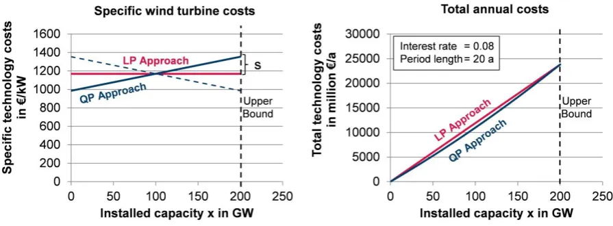
in linear models equal a constant average value, in the quadratic programming (QP) model the entire cost range described in the investment cost chapter is distributed over the installable capacity of the technology. The upper bound of the capacity variable can be either the technical potential of a technology or its expansion limit at a specific time interval. In the depicted case, the cheapest units of the technology are sold first (blue curve). This is supported by the assumption of free markets. In theory, it is also possible to implement the cost range and vice versa (dashed line), for example to consider learning curves. However, this implicates local optima in the optimisation process and cannot be solved by the solvers mentioned above. Instead, piecewise linearization can be used for an approximation of this problem.[32]

Figure 2. Comparison of the consideration of investment costs in the LP (red) and QP model (blue).

The objective function of the modified linear models is intended to minimise the total annual system costs. These costs are divided into fixed and variable costs. The fixed costs consist of CAPEX and fixed operational expenditures (fixed OPEX) mfix. For the determination of the CAPEX of a specific technology y, the capital recovery factor r is utilised based on interest rate i and the number of periods n (Equation 1):

𝑟_{𝑛,𝑖,𝑦}= (1 + 𝑖)

𝑛_{∙ 𝑖}

(1 + 𝑖)𝑛_{− 1} (1)

In the linear case, the specific technology costs, kLP, are constant and independent of the installed capacity x (Equation 2). They are based on an average cost value, C0, or a forecasted value for future scenarios. This factor, multiplied by the capital recovery factor and the fixed OPEX as a percentage of C0 results in the fixed costs αLPfix (Equation 3):

𝑘𝐿𝑃(𝑥𝑦) = 𝐶0,𝑦 (2)

𝛼_{𝐿𝑃𝑓𝑖𝑥}(𝑥_𝑦) = 𝐶_0,𝑦∙ (𝑟_{𝑛,𝑖,𝑦}+ 𝑚_{𝑓𝑖𝑥,𝑦}) (3)

Consequently, the total fixed annual costs KLPfix are integral of αLPfix between the lower xlb and upper bound xub of the capacity of technology y (equations 4 and 5):

𝐾_{𝐿𝑃𝑓𝑖𝑥}(𝑥_𝑦) = ∫ 𝛼_{𝐿𝑃𝑓𝑖𝑥}(𝑥_𝑦)

𝑥𝑢𝑏,𝑦

𝑥𝑙𝑏,𝑦

𝑑𝑥_𝑦 (4)

The variable costs are based on energy and material flows, k, of the energy system in time step, t, which are allocated to the technologies by the ingoing and outgoing flows, ẋ. In combination with the total fixed annual costs, the objective function can be expressed, as follows, in Equation 6:

𝑚𝑖𝑛 𝑓(𝑥) = 𝑚𝑖𝑛 ∑ 𝐶_0,𝑦∙ (𝑟_{𝑛,𝑖,𝑦}+ 𝑚_{𝑓𝑖𝑥,𝑦}) ∙ 𝑥_𝑦

𝑦𝜖𝑌

+ ∑ ∑ 𝑚_{𝑣𝑎𝑟,𝑘}∙ 𝑥̇_𝑘,𝑡

t∈𝑻

𝑘∈𝑲 (6)

In contrast to the linear approach, the specific cost function of the QP model kQP(xy) has a constant slope, v. Moreover, the average cost value, C0, can be replaced by the weighted average value in Figure 1. The impact on the fixed costs, αQPfix,is explained in equations 7-9:

𝑣 =𝑑𝑘

𝑑𝑥 = 𝑐𝑜𝑛𝑠𝑡 (7)

𝑘_𝑄𝑃(𝑥_𝑦) = 𝑣_𝑦∙ 𝑥_𝑦+ 𝐶_0,𝑦−1

2𝑣𝑦∙ (𝑥𝑢𝑏,𝑦− 𝑥𝑙𝑏,𝑦) (8)

𝛼𝑄𝑃𝑓𝑖𝑥(𝑥𝑦) = 𝑘𝑄𝑃(𝑥𝑦) ∙ (𝑟𝑛,𝑖,𝑦+ 𝑚𝑓𝑖𝑥,𝑦) (9)

On the basis of these equations, the total fixed annual costs, KQPfix, are described in equations 10 and 11:

𝐾_𝑄𝑃(𝑥_𝑦) = ∫ 𝛼_{𝑄𝑃𝑓𝑖𝑥}(𝑥_𝑦)

𝑥𝑢𝑏,𝑦

𝑥𝑙𝑏,𝑦

𝑑𝑥_𝑦 (10)

𝐾_𝑄𝑃(𝑥_𝑦) = [1₂𝑣_𝑦∙ 𝑥_𝑦2_{+ 𝐶}

0,𝑦∙ 𝑥𝑦−

1

2𝑣𝑦∙ (𝑥𝑢𝑏,𝑦− 𝑥𝑙𝑏,𝑦) ∙ 𝑥𝑦] ∙ (𝑟𝑛,𝑖,𝑦+ 𝑚𝑓𝑖𝑥,𝑦) (11) As the declaration of the specific cost slope is not especially common, the equation can be simplified by introducing the absolute deviation, s, of the minimum or maximum cost value from the average or weighted average cost value (see Figure 2). This leads to equation 12 for the definition of specific costs, kQP. Its consequences to the total fixed annual costs are shown in equations 13 and 14:

𝛼_{𝑄𝑃𝑓𝑖𝑥}(𝑥_𝑦) = 𝐶_0,𝑦∙ [(1 − 𝑠_𝑦) + 2𝑠𝑦

𝑥_{𝑢𝑏,𝑦}− 𝑥_{𝑙𝑏,𝑦}∙ 𝑥𝑦] ∙ (𝑟𝑛,𝑖,𝑦+ 𝑚𝑓𝑖𝑥,𝑦) (12)

𝐾_𝑄𝑃(𝑥_𝑦) = ∫ 𝛼_{𝑄𝑃𝑓𝑖𝑥}(𝑥_𝑦)

𝑥𝑢𝑏,𝑦

𝑥𝑙𝑏,𝑦

𝑑𝑥_𝑦 (13)

𝐾_𝑄𝑃(𝑥_𝑦) = [𝐶_0,𝑦∙ (1 − 𝑠_𝑦) ∙ 𝑥_𝑦+ 𝐶0,𝑦∙ 𝑠𝑦

𝑥_{𝑢𝑏,𝑦}− 𝑥_{𝑙𝑏,𝑦}∙ 𝑥𝑦2] ∙ (𝑟𝑛,𝑖,𝑦+ 𝑚𝑓𝑖𝑥,𝑦) (14) The final objective function of the QP model is shown in equation 15:

𝑚𝑖𝑛 𝑓(𝑥) = 𝑚𝑖𝑛 ∑ [𝐶_0,𝑦∙ (1 − 𝑠𝑦) ∙ 𝑥𝑦+

𝐶0,𝑦∙ 𝑠𝑦

𝑥_{𝑢𝑏,𝑦}− 𝑥_{𝑙𝑏,𝑦}∙ 𝑥𝑦2] ∙ (𝑟𝑛,𝑖,𝑦+ 𝑚𝑓𝑖𝑥,𝑦)

𝑦𝜖𝑌

+ ∑ ∑ 𝛼_{𝑣𝑎𝑟,𝑘}∙ 𝑥̇_𝑘,𝑡

t∈𝑻 𝑘∈𝑲

(15)

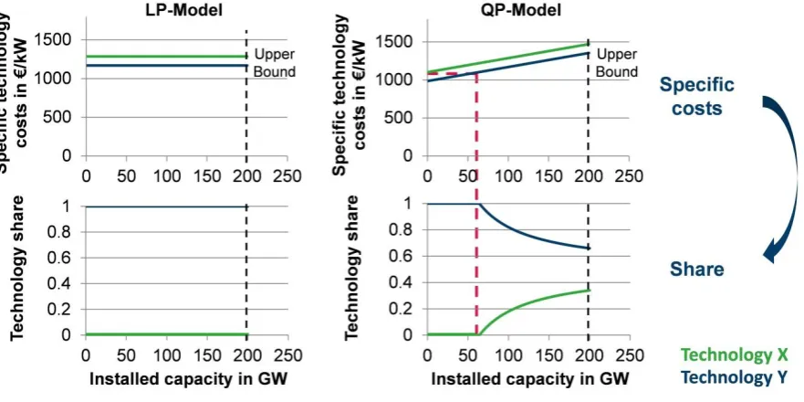
change the result. Otherwise, in the QP approach both technologies would be in the solution if demand is high enough. The closer the specific cost values of the technologies, the more congruent their shares in the energy system are. As a consequence, the Penny Switching Effect can be avoided and the results become more robust.

Figure 3. Qualitative comparison of two similar technology shares in the optimised solution of the LP and QP model.

5. Comparison of linear and quadratic programming results

The corroboration of the hypothesis requires verification through an appropriate testing model. For verification purposes, a linear programming model for minimisation of the total energy system costs for Germany is chosen. Its temporal resolution is set to one hour, aggregated to 24 typical days.[17, 18] Spatial aspects are not considered. In this context, a potential energy system for the target year of 2050 is optimised for an 80% CO2 emission reduction scenario, in accordance with the German ‘Klimaschutzplan 2050’.[33] A detailed description of the model can be found in the methods section.

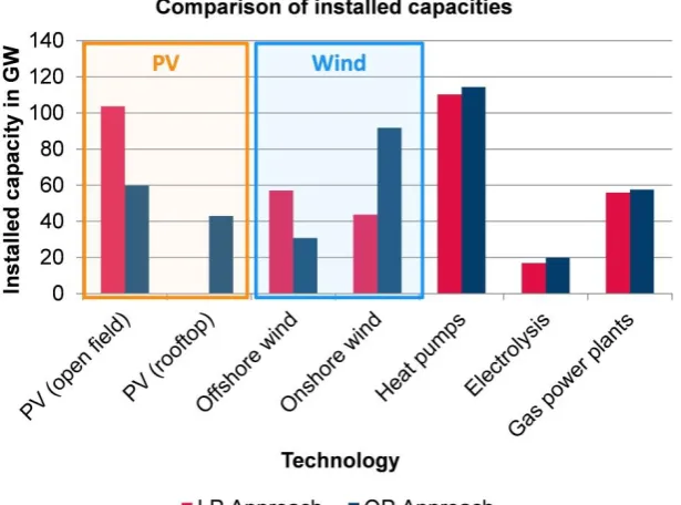
Figure 4. Comparison of installed capacities in the results of the LP (red) and QP (blue) model for an 80% CO2 emission reduction scenario for Germany.

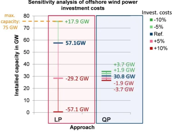
Figure 5. Sensitivity analysis of the investment costs for offshore wind turbines and its impact on the installed capacity in the cost-optimised energy system in the LP and QP model.

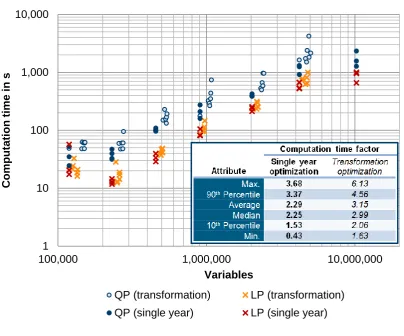
Figure 6. Comparison of computation time of different LP and QP problems

6. Discussion and conclusions

The preceding analysis showed that technological investment costs generally vary across wide ranges and the predictions of future trends are subject to uncertainties. Nevertheless, these cost ranges can be incorporated and simplified by implementing a quadratic objective function in conventional energy system optimisation models. In particular, models with the purpose of evaluating greenhouse gas reduction strategies that implement high shares of renewable energy in the system benefit from this approach. The investigation reveals that the results of the modified model become more robust and a broader mix of technologies is considered in the solution. Instead of penny switching effects in the LP model, the technology shares are affected much less by a variation in the specific investment costs. Moreover, when comparing the results shown in Figure 4 to the current energy system of Germany, the installed capacities of wind power and PV follow actual trends. Thus, the solution better reflects the present investment behaviour and might be described as more realistic. However, there are two effects of the QP approach that must also be discussed. Concerning the resulting total system costs, the calculated costs of the QP model are systematically lower than in the LP model if the same average value of the investment costs is implemented. This can be attributed to the fact that the average total investment costs of a technology are only equal to the linear case if the installed capacity reaches its upper bound (compare Figure 2). Either this effect is assigned to market behaviour and justified by the point of the improved implementation of markets or must be corrected by the real average

1 10 100 1,000 10,000

100,000 1,000,000 10,000,000

C

ompu

tati

on

t

ime

in

s

Variables

Comparison of computation time

QP (transformation) LP (transformation)

cost value after optimisation. Aside from this effect, the results of the QP model are influenced by the definition of the specific investment cost ranges themselves. This means that the determination of the considered range, as well as the span between the lower and upper bound of installable capacity affects the result. The wider the cost range and the closer the lower and upper bound, the more the gradient of the specific technology cost curve increases. Consequently, the shares of alternative technologies become more even. This must be taken into consideration when evaluating the results.

Appendix

Table 1. Summary of decisive techno-economic input parameters of the model.[26, 34-37]

Component Specific invest. costs in €/kW Cost range in percentage deviation Level of efficiency

CO2 emissions in gCO2/kWh

Name Today 2050 Today 2050 Today 2050 Today 2050

Photovoltaics

(rooftop) 1500 880 ±23% ±14% (1)* (1)* 0 0

Photovoltaics

(open field) 1100 720 ±9% ±11% (1)* (1)* 0 0

Onshore wind

power 1850 1250 ±30% ±36% (1)* (1)* 0 0

Offshore wind

power 3920 2530 ±21% ±29% (1)* (1)* 0 0

Coal power

station 1600 1600 ±9% ±9% 0.45 0.48 890 840

Lignite power

station 2050 2050 ±17% ±17% 0.42 0.47 1010 910

Gas power

station 550 550 ±27% ±27% 0.40 0.45 575 510

Biomass

power station 3200 2080 ±22% ±21% 0.34 0.38 (0)** (0)**

Hydropower

station 5250 5370 ±52% ±52% (1)* (1)* 0 0

Pumped hydro

storage 3000 3000 ±50% ±50% 0.8*** 0.9*** 0 0

Battery storage (Li)

752

(€/kWh)

246

(€/kWh) ±20% ±20% 0.9*** 0.9*** 0 0

Hydrogen cavern storage

0.52

(€/kWh)

0.52

(€/kWh) ±0% ±0% 1 1 0 0

Electrolyser

(PEM) 1564 500 ±21% ±21% 0.69 0.7 0 0

Fuel cell (PEM) 3650 923 ±4% ±4% 0.49 0.5 0 0

Heat pumps 800

(€/kWel)

645

(€/kWel) ±38% ±38%

3.0

(COP)

3.5

(COP) 0 0

* Assumption based on the calculation of the primary energy consumption of Germany[38]

** Assumption of neutral CO2 emissions based on the calculation of the national greenhouse gas emissions of

Germany[39]

*** Round-trip efficiency

The model’s structure and parameters were validated based on historical data from the year 2013 in accordance with the integrated supply and demand profiles.

References

[1] Lopion P, Markewitz P, Robinius M, Stolten D. A review of current challenges and trends in energy systems modeling. Renewable and Sustainable Energy Reviews. 2018;96:156-66. [2] Van Beeck N. Classification of energy models: Tilburg University, Faculty of Economics and Business Administration; 2000.

[3] Hall LMH, Buckley AR. A review of energy systems models in the UK: Prevalent usage and categorisation. Applied Energy. 2016;169:607-28.

[4] Pfenninger S, Hawkes A, Keirstead J. Energy systems modeling for twenty-first century energy challenges. Renewable and Sustainable Energy Reviews. 2014;33:74-86.

[5] Anadón LD, Baker E, Bosetti V. Integrating uncertainty into public energy research and development decisions. Nature Energy. 2017;2:17071.

[6] Ma T, Nakamori Y. Modeling technological change in energy systems – From optimization to agent-based modeling. Energy. 2009;34:873-9.

[7] McCollum DL, Zhou W, Bertram C, de Boer H-S, Bosetti V, Busch S, et al. Energy investment needs for fulfilling the Paris Agreement and achieving the Sustainable Development Goals. Nature Energy. 2018;3:589-99.

[8] Winskel M. Beyond the disruption narrative: Varieties and ambiguities of energy system change. Energy Research & Social Science. 2018;37:232-7.

[9] Gritsevskyi A, Nakićenovi N. Modeling uncertainty of induced technological change. Energy Policy. 2000;28:907-21.

[10] Schmidt O, Hawkes A, Gambhir A, Staffell I. The future cost of electrical energy storage based on experience rates. Nature Energy. 2017;2:17110.

[11] Held AM. Modelling the future development of renewable energy technologies in the European electricity sector using agent-based simulation: Fraunhofer Verlag; 2011. [12] Kovacevic RM, Pflug GC, Vespucci MT. Handbook of risk management in energy production and trading: Springer; 2013.

[13] Pfluger B. Assessment of least-cost pathways for decarbonising Europe's power supply: a model-based long-term scenario analysis accounting for the characteristics of renewable energies: KIT Scientific Publishing; 2014.

[14] Connolly D, Lund H, Mathiesen BV, Leahy M. A review of computer tools for analysing the integration of renewable energy into various energy systems. Applied Energy.

2010;87:1059-82.

[15] Bosetti V, Marangoni G, Borgonovo E, Diaz Anadon L, Barron R, McJeon HC, et al. Sensitivity to energy technology costs: A multi-model comparison analysis. Energy Policy. 2015;80:244-63.

[16] Seljom P, Tomasgard A. Short-term uncertainty in long-term energy system models — A case study of wind power in Denmark. Energy Economics. 2015;49:157-67.

[17] Kotzur L, Markewitz P, Robinius M, Stolten D. Time Series Aggregation for Energy System Design: Modeling Seasonal Storage. arXiv preprint arXiv:171007593. 2017.

[18] Kotzur L, Markewitz P, Robinius M, Stolten D. Impact of different time series aggregation methods on optimal energy system design. Renewable Energy. 2018;117:474-87.

[19] Bürger V, Hesse T, Quack D, Palzer A, Köhler B, Herkel S, et al. Klimaneutraler Gebäudebestand 2050. On behalf of the German Environment Agency Climate Change. 2016;6:2016.

[20] Gerbert P, Herhold P, Burchardt J, Schönberger S, Rechenmacher F, Kirchner A, et al. Klimapfade für Deutschland. Bundesverbandes der Deutschen Industrie (BDI). 2018. [21] Renewable Power Generation Costs in 2017. IRENA (2018), International Renewable Energy Agency, Abu Dhabi. 2018.

[22] Drechsler M, Egerer J, Lange M, Masurowski F, Meyerhoff J, Oehlmann M. Efficient and equitable spatial allocation of renewable power plants at the country scale. Nature Energy. 2017;2:17124.

[23] Afanasyeva S, Saari J, Kalkofen M, Partanen J, Pyrhönen O. Technical, economic and uncertainty modelling of a wind farm project. Energy Conversion and Management.

[24] Rout UK, Blesl M, Fahl U, Remme U, Voß A. Uncertainty in the learning rates of energy technologies: An experiment in a global multi-regional energy system model. Energy Policy. 2009;37:4927-42.

[25] Pure power-wind energy targets for 2020 and 2030: Ewea, European Wind Energy Association; 2011.

[26] Carlsson J. Energy Technology Reference Indicator projections for 2010-2050. European Commission, Joint Research Centre, Institute for Energy and Transport Luxembourg. 2014;10:057687.

[27] Roadmap E. 2050: a practical guide to a prosperous, low carbon Europe. Brussels: ECF. 2010.

[28] Taylor M, Ralon P, Ilas A. The power to change: solar and wind cost reduction potential to 2025. International Renewable Energy Agency (IRENA). 2016.

[29] MacDonald M. Costs of low-carbon generation technologies. Report for the Committee on Climate Change Brighton, Mott MacDonald. 2011.

[30] Creutzig F, Agoston P, Goldschmidt JC, Luderer G, Nemet G, Pietzcker RC. The underestimated potential of solar energy to mitigate climate change. Nature Energy. 2017;2:17140.

[31] McCollum DL, Jewell J, Krey V, Bazilian M, Fay M, Riahi K. Quantifying uncertainties influencing the long-term impacts of oil prices on energy markets and carbon emissions. Nature Energy. 2016;1:16077.

[32] Heuberger CF, Rubin ES, Staffell I, Shah N, Mac Dowell N. Power capacity expansion planning considering endogenous technology cost learning. Applied Energy. 2017;204:831-45.

[33] Bundesministerium für Umwelt N, Bau und Reaktorsicherheit. Klimaschutzplan 2050– Klimapolitische Grundsätze und Ziele der Bundesregierung. 2016.

[34] Saba SM, Müller M, Robinius M, Stolten D. The investment costs of electrolysis – A comparison of cost studies from the past 30 years. International Journal of Hydrogen Energy. 2018;43:1209-23.

[35] Noack C, Burggraf F, Hosseiny S, Lettenmeier P, Kolb S, Belz S, et al. Studie über die Planung einer Demonstrationsanlage zur Wasserstoff-Kraftstoffgewinnung durch Elektrolyse mit Zwischenspeicherung in Salzkavernen unter Druck. German Aerospace Center:

Stuttgart, Germany. 2015.

[36] Welder L, Ryberg DS, Kotzur L, Grube T, Robinius M, Stolten D. Spatio-temporal optimization of a future energy system for power-to-hydrogen applications in Germany. Energy. 2018;158:1130-49.

[37] Stolzenburg K, Hamelmann R, Wietschel M, Genoese F, Michaelis J, Lehmann J, et al. Integration von Wind-Wasserstoff-Systemen in das Energiesystem. Analysis on behalf of Nationale Organisation Wasserstoff-und Brennstoffzellentechnologie GmbH (NOW). 2014. [38] Energiebilanzen 1990-2016. Berlin, Germany: AGEB1990.

[39] Harthan RO, Hermann H. Sektorale Abgrenzung der deutschen